Universidade do Minho
Escola de Engenharia Departamento de Inform´atica
Marta Vasconcelos Castro Azevedo
Correct Translation of Imperative Programs
to Single Assignment Form
Universidade do Minho
Escola de Engenharia Departamento de Inform´atica
Marta Vasconcelos Castro Azevedo
Correct Translation of Imperative Programs
to Single Assignment Form
Master dissertation
Master Degree in Computer Science
Dissertation supervised by
Professor Maria Jo ˜ao Frade Professor Lu´ıs Pinto
A B S T R A C T
A common practice in compiler design is to have an intermediate representation of the source code in Static Single-Assignment (SSA) form in order to simplify the code optimization process and make it more efficient. Generally, one says that an imperative program is in SSA form if each variable is assigned exactly once.
In this thesis we study the central ideas of SSA-programs in the context of a simple imperative lan-guage including jump instructions. The focus of this work is the proof of correctness of a translation from programs of the source imperative language into the SSA format. In particular, we formally intro-duce the syntax and the semantics of the source imperative language (GL) and the SSA language; we define and implement a function that translates from source imperative programs into SSA-programs; we develop an alternative operational semantics, in order to be able to relate the execution of a source program and of its SSA translation; we prove soundness and completeness results for the translation, relatively to the alternative operational semantics, and from these results we prove correctness of the translation relatively to the initial small-step semantics.
R E S U M O
Uma pr´atica comum no design de compiladores ´e ter uma representac¸˜ao interm´edia do c´odigo fonte em formato Static Single Assigment (SSA), de modo a facilitar o processo subsequente de an´alise e optimizac¸˜ao de c´odigo. Em termos gerais, diz-se que um programa imperativo est´a no formato SSA se cada vari´avel do programa ´e atribu´ıda exatamente uma vez.
Nesta tese estudamos as ideias principais do SSA no contexto de uma linguagem imperativa simples com instruc¸˜oes de salto. O foco deste trabalho ´e a prova de correcc¸˜ao de uma traduc¸˜ao dos programas fonte para formato SSA. Concretamente, definimos formalmente a sintaxe e a semˆantica da linguagem fonte (GL) e da linguagem em formato SSA; definimos e implementamos a func¸˜ao de traduc¸˜ao; desen-volvemos semˆanticas operacionais alternativas de modo a permitir relacionar a execuc¸˜ao do programa fonte com a sua traduc¸˜ao SSA; provamos a idoneidade e a completude do processo de traduc¸˜ao relati-vamente `as semˆanticas alternativas definidas; e a partir destes resultados demostramos a correcc¸˜ao da traduc¸˜ao em ordem `as semˆanticas operacionais estruturais definidas inicialmente.
C O N T E N T S
1 I N T R O D U C T I O N 2
1.1 Imperative and functional programming 2
1.2 Compilation process 3
1.3 Single assignment form 4
1.4 Continuation passing style 6
1.5 Contributions and document structure 7
2 I M P E R AT I V E L A N G U A G E A N D S I N G L E A S S I G N M E N T F O R M 9
2.1 The Goto LanguageGL 9
2.1.1 Syntax 10
2.1.2 Semantics 12
2.2 SA language 15
2.2.1 Syntax 15
2.2.2 Operational semantics in SA programs 17
3 A T R A N S L AT I O N I N T O S A F O R M 20
3.1 Translating into SA form 20
4 C O R R E C T N E S S O F T H E T R A N S L AT I O N I N T O S A F O R M 27
4.1 Splitting the transition relation of the source languageGL 27
4.1.1 Computation inside block 27
4.1.2 Computation across blocks 28
4.2 Splitting the transition relation in the SA language 31
4.2.1 Computation inside blocks 31
4.2.2 Computation across blocks 32
4.3 Properties of the translation into SA form 35
4.3.1 Soundness 36
4.3.2 Completeness 40
4.3.3 Correctness 46
5 F I N A L R E M A R K S 48
5.1 SA Translation 48
5.1.1 Optimal placement of φ-functions 48
5.1.2 Adapting the translation functionT 50
5.2 Relation with Functional Programming 52
5.3 Conclusions and Future Work 54
Contents
L I S T O F F I G U R E S
Figure 1 Example of a imperative program 3
Figure 2 Example of a functional program 3
Figure 3 Translation in a simple program in SA 4
Figure 4 Example of a transformation into SSA form 6 Figure 5 CFG corresponding to example presented in Figure 1 6
Figure 6 Translation into SA format 21
Figure 7 FunctionRand its auxiliary functions 22
Figure 8 Functions sync andS 23
Figure 9 FunctionT 23
Figure 10 Program sum and its CFG 49
Figure 11 Translation into SA format withOP 50
Figure 12 FunctionRand its auxiliary functions 51
Figure 13 FunctionS 51
Figure 14 FunctionT 52
L I S T O F A B B R E V I AT I O N S
CPS Continuation Passing Style SA Single Assignment
SSA Static Single Assignment CFG Control Flow Graph
1
I N T R O D U C T I O N
1.1 I M P E R AT I V E A N D F U N C T I O N A L P R O G R A M M I N G
A programming language is a notation for writing programs, which are specifications of a computation to be performed by a machine. Different approaches to programming have been developed over time. There are many different programming paradigms that allow the possibility to determine the programmer’s view of the problem. Despite some languages are designed to support one particular paradigm, there are others that support multiple paradigms.
This work focuses on two of these paradigms, which have drawn programmers and computer scien-tists’ attention since early times: the imperative programming paradigm and the functional program-ming paradigm. Both paradigms are built upon different ideas.
In imperative languages computation is specified in an imperative form (i.e., as a sequence of operations to perform). The model of computation in the imperative paradigm relies on the notion of state(seen as the content of the program variables which represent storage/memory locations, at any given point in the program’s execution ) and statements/commands that change a program’s state. So, an imperative program consists of a sequence of commands for the computer to perform. A program describes how a program operates. In Figure1 we can see a snippet of a imperative program. This program sums all the numbers from0 to n.
The first imperative programming languages were machine languages with simple instructions. Gradually, some more complex languages were introduced such as C, Pascal or Java.
Contrasting with imperative programming, functional programming focuses on what the program should accomplish without specifying how the program should achieve the result. Functional program-ming has its roots in λ-calculus (Church,1932). The functional programming paradigm is based on the notion of mathematical function (a program is a collection of functions) and program execution corresponds to the evaluation of expressions (involving the functions defined in the program). Func-tional programs deal only with mathematical variables (the formal arguments of the functions). The output value of a function depends only on the arguments that are inputs to the function. So, calling a function twice with the same argument values will produce the same result each time. This property is called referential transparency and make it much easier to understand and predict the behavior of a program.
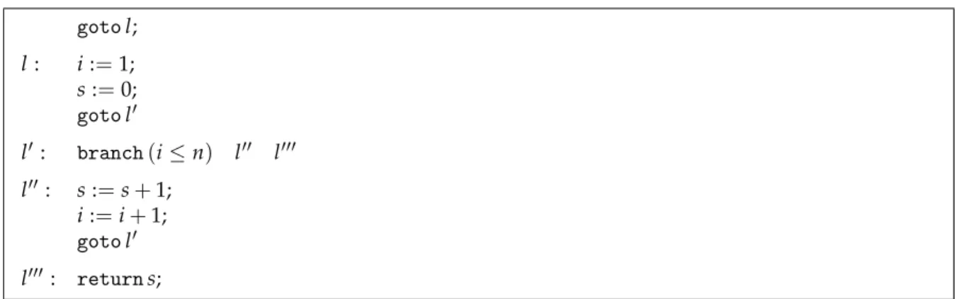
1.2. Compilation process gotol; l : i :=1; s :=0; gotol0 l0 : branch(i≤n) l00 l000 l00: s :=s+1; i :=i+1; gotol0 l000 : returns;
Figure 1.: Example of a imperative program
Note that in imperative programming, as for instance in C, one usually call “functions” to subrou-tines that are not really functions (in the mathematical sense), since they can have side effects that may change the value of the program state and the value they produce may depend on the state also. Be-cause of this, they lack referential transparency, i.e. the same language expression may have different values at different times depending on the state of the program.
An expression is said to be referentially transparent if it can be replaced with its value without changing the behavior of a program. This allows the programmer and the compiler to reason about program behavior as a rewrite system, and is very helpful in the static analysis of the code, proving its correctness or optimizing it.
Functional programming languages have long been popular in academia. More recently, several functional programming languages are being used in industry and became popular for building a range of applications. The first functional-flavoured language was Lisp (developed in 1950s). Since then many different languages emerged (some of them multi-paradigm). Scheme, SML, Ocaml and Haskell are examples of more recent functional programming languages..
We can see, in Figure2a program fragment in Haskell with the functional approach to the sum function displayed on Figure1.
fun:: Int→Int
fun n=ifn≤0 then 0 else n+ (funn−1)
Figure 2.: Example of a functional program
1.2 C O M P I L AT I O N P R O C E S S
For a computer to be able to execute the instructions given by a program written in a (high-level) pro-gramming language, it is necessary to translate the source program into an equivalent target program in machine language (for the specific hardware). This translation is the task of the compiler.
1.3. Single assignment form
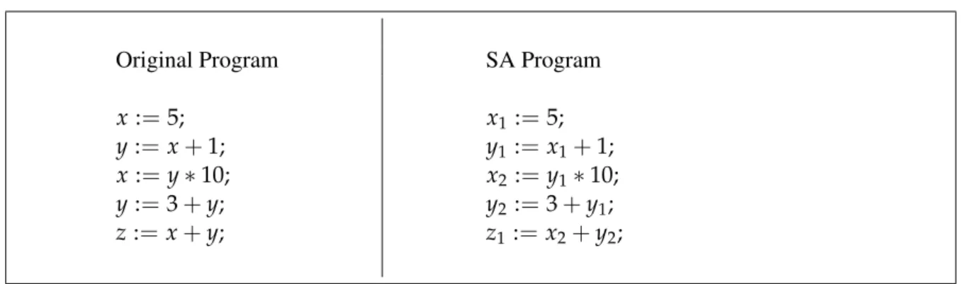
Original Program SA Program
x :=5; x1:=5;
y := x+1; y1 := x1+1;
x :=y∗10; x2:=y1∗10;
y :=3+y; y2 :=3+y1;
z := x+y; z1:= x2+y2;
Figure 3.: Translation in a simple program in SA
Compilers are complex programs that are organized in several phases usually grouped as follows: The front-end performs the syntactic and semantic processing and generates an intermediate repre-sentation of the source code to be then processed by the middle-end. The middle-end performs opti-mizations over the intermediate code generates another intermediate representation for the back-end. The back-end performs more analysis and optimizations for a particular hardware and then generates machine code for a particular processor and operating system. This approach makes it possible to combine front ends for different languages with back ends for different hardware. Examples of this approach are the GNU Compiler Collection (Stallman,2001) and LLVM (Lattner and Adve,2004), which have multiple front-ends, shared analysis and multiple back-ends.
In compiler design, a common practice is to have the intermediate representation of the source code in static single assignment form in order to simplify the code optimization process.
Another style used as an intermediate representation to perform optimizations and program trans-formations is the continuation-passing style. Despite continuations can be used to compile most pro-gramming languages they are more common on the compilation process of functional languages.
1.3 S I N G L E A S S I G N M E N T F O R M
One says that an imperative program is in static single assignment (SSA) form if each variable is assigned exactly once, and every variable is defined before it is used. This restriction makes explicit in the program syntax the link between the program point where a variable is defined and read.
Converting into SSA form is usually done splitting the (original) variables into “versions”, with the new variables typically denoted by the original name with an index, so that every definition gets its own version. The transformation of a program into SSA form has to be semantic preserving. One simply tags each variable definition with an index, and each variable use with the index corresponding to the last definition of this variable. You can see an example in Figure3.
This transformation preserves the semantics of the program in the sense that the final values ofx, y andz in the first program coincide with the values of the final vertions of those variables: x2,y2andz1.
1.3. Single assignment form
The SSA form was introduced in the 1980s by Ron Cytron et al (Cytron et al., 1991) and it is a popular intermediate representation for compiler optimizations. The considerable strength of the SSA form, where variables are statically assigned exactly once, simplifies the definition of many optimizations, and improves their efficiency and the quality of their results. The SSA format plays a central role in a range of optimization algorithms relying on data flow information, and hence, to the correctness of compilers employing those algorithms. Examples of optimization algorithms which benefit from the use of SSA form include, among others, constant propagation, value range propagation, dead code elimination and register allocation. Many modern optimizing compilers, such as the GNU Compiler Collection and LLVM Compiler Infrastructure rely heavily on SSA form.
The apparent simplicity of the SSA conversion of the code snippet example given above is mis-leading. For program with control flow commands (for instance, if and while or goto commands) the translation to SSA form cannot be done solely by tagging variables: to handle it one must insert the so-called φ-functions, which control the merging of data flow edges entering code blocks. For instance, where two control-flow edges join together, carrying different values of some variable, one must somehow merge the two values. This is done with the help of a φ-function, which is a notational trick. In some node with two in-edges, the expression φ(a, b)has the valuea if one reaches this node on the first in-edge, andb if one comes in on the second in-edge. The semantics of φ-functions is in the seminal paper byCytron et al.(1991):
”If control reaches nodej from its kth predecessor, then the run-time support remembers k while executing the φ-functions in j. The value of φ(x1, x2, ...)is just the value of the
kth operand. Each execution of a φ-function uses only one of the operands, but which one depends on the flow of control just before enteringj.”
Let us illustrate the translation to SSA form with an example in Figure4.
There may be several SSA forms for a single control-flow graph program. As the number of φ-functions directly impacts size of the SSA form and the quality of the subsequent optimisations it is important that SSA generators for real compilers produce a SSA form with a minimal number of
φ-functions. Implementations of minimal SSA generally rely on the notion of dominance frontier to
choose where to insert φ-functions, as indicated, for instance, in (Cytron et al.,1991).
The Control Flow Graph (CFG) is a representation, using graph notation, of all paths that might be traversed a program during execution. In a CFG, node A dominates node B if any path from the start to node B must go though A. There is a vast body of work on efficient methods of computing min-imal SSA form and SSA-based optimisations. General references are Appel(1998b) andMuchnick
1.4. Continuation passing style
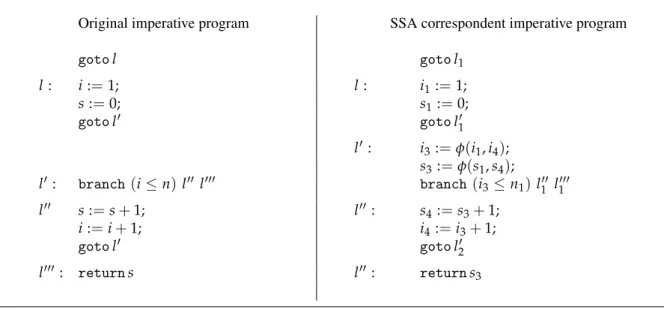
Original imperative program SSA correspondent imperative program
gotol gotol1 l : i :=1; l : i1:=1; s :=0; s1:=0; gotol0 gotol10 l0: i3:=φ(i1, i4); s3:=φ(s1, s4); l0: branch (i≤n)l00 l000 branch(i3≤n1) l001 l0001 l00 s :=s+1; l00: s4:=s3+1; i :=i+1; i4:=i3+1; gotol0 gotol20 l000 : returns l00: returns3
Figure 4.: Example of a transformation into SSA form
Figure 5.: CFG corresponding to example presented in Figure1
1.4 C O N T I N U AT I O N PA S S I N G S T Y L E
In the functional paradigm, continuation-passing style (CPS) is a style of programming in which control is passed explicitly in the form of a continuation. This is not the style usually used by pro-grammers (generally called the direct style). Continuation-passing style is used as an intermediate representation to perform optimisations and program transformations. CPS has been used as an inter-mediate language in compiler for functional languages, seeAppel(2007).
1.5. Contributions and document structure
A function written in CPS takes an extra argument, the continuation function, which is a function of one argument. When the CPS function comes to a result value, it returns it by calling the continuation function with this value as the argument. The continuation represents what should be done with the result of the function being calculated. This feature, along with some other restrictions on the form of expressions, makes a number of things explicit (such as function returns, intermediate values, the order of argument evaluation and tail calls) which are implicit in direct style. λ-calculus in CPS, as an intermediate representation, is used to expose the semantics of programs, making them easier to analyze and the optimization process more efficient for functional-language compilers.
It is well known that the SSA form is closely related to λ-terms . (Kelsey, 1995) pointed to a correspondence between programs in SSA form and λ-terms in CPS. In CPS there is exactly one binding form for every variable and variable uses are lexically scoped. In SSA there is exactly one assignment statement for every variable and that statement dominates all uses of the variable.
InKelsey(1995), Kelsey define syntactic transformation that convert CPS programs into SSA and vice-versa. Some CPS programs cannot be converted to SSA but these are not pro duced by the usual CPS transformation. The transformations from CPS into SSA is especially helpful for compiling func-tional programs. Many optimizations that normally require flow analysis can be performed directly on functional CPS programs by viewing them as SSA programs.
1.5 C O N T R I B U T I O N S A N D D O C U M E N T S T R U C T U R E
In this work we study the central ideas of static single assignment programs in a context of a simple imperative language including jump instructions. The fundamental contribution of this thesis is the proof of correctness of a translation from programs of the base imperative language into the SSA format. In particular,
• we defined small-step operational semantics for the base imperative language and for the corre-sponding SSA language;
• we defined a translation from programs of the base language into SSA-programs, and proto-typed it in Haskell inhttps://goo.gl/PtfqGJ;
• we developed alternative operational semantics, both for the base imperative language and for the SSA language, which split the computation, according to whether it involves a jump or not, and keeps track of information about the variables in order to identify the adequate version of each variable, when relating execution of a base program and of its SSA translation;
• we proved each of these alternative semantics equivalent to the corresponding small-step se-mantics;
1.5. Contributions and document structure
• we proved soundness and completeness results for the translation, relatively to the alternative operational semantics, and from these results we proved correctness of the translation relatively to the initial small-step semantics.
The thesis is organized as follows: In Chapter 2 we formally introduce the syntax and the semantics of the base imperative language and the SSA language that are used in this work. In Chapter 3 we present in every detail a function that translates from base imperative programs into SSA-programs. Chapter 4 is entirely devoted to the proof of correctness of the translation defined. In Chapter 5 we discuss some possible improvements to the translation function and the relation of SSA-programs and the functional programming paradigm. Finally we draw some conclusions and directions for future work.
2
I M P E R AT I V E L A N G U A G E A N D S I N G L E A S S I G N M E N T F O R M
In this chapter we introduce a base imperative language and a SSA language that will be used in our study. For the sake of simplicity we will refer to SSA format just as SA form. We will callGL(short for Goto Language) to the imperative language. Let us begin by introducing some general notation used for functions and lists.
N O TAT I O N: Given a function f , dom ( f ) denotes the domain of f and f[x 7→ a] denotes the function that maps x to a and any other value y to f(y). We also use the notation[x 7→ g(x)| x ∈
A] to represent the function with domain A generated by g. For a set B ⊆ dom(f), f(B) = {f(x) | x ∈B}.
For every A, we let A∗denote the set of lists of elements ofA, and[ ]denote the empty list.~a ranges overA+, ifa ranges over A. #~a denotes the length of~a.~a[n]withn≤#~a denotes the nthelement of~a. For convenience, we will sometimes write non-empty lists in the formh : t, where h denotes the first element of the list (its head) andt the rest of it (its tail).
We use the++ infix operator for the concatenation of two lists.
Given a total function f : X → Y and a partial function g : X * Y, we define f ⊕g : X → Y as follows:
(f⊕g)(x) =
(
g(x) if x∈dom(g)
f(x) if x6∈dom(g)
i.e.,g overrides f but leaves f unchanged at points where g is not defined.
2.1 T H E G O T O L A N G U A G E G L
G Lis a simple “goto” language whose programs are defined as sequences of labeled blocks with an entry point. Blocks are sequences of assignments that end with a jump or a return instruction, if the program ends in the block. Labels are used as names for the blocks.
2.1. The Goto LanguageGL
2.1.1 Syntax
For our imperative language, G L, we have various categories and for each one we have meta-variables that will be used to range over constructs of each category. N u m denotes numerals, i.e. , some set of encoding of integers and we will have letter n to range over N u m . Va r denotes a set of variables which is assumed to be infinite. Small letters such as x , y, z, ... will denote variables and range over Va r . To represent the labels, we have l, l0, l0 0... that will range over L (set of all the labels). Finally, A e x p represents the set of arithmetic expressions and C e x p the set of
condi-tional expressions. The abstract syntax for arithmetic and condicondi-tional expressions is presented in the following definition:
Definition 1 (Abstract syntax for Expressions) Forx ∈ Va r and n ∈ N u m : A e x p 3 a : := n | x | a +a0 | a ×a0 | a −a0
C e x p 3 c : := ¬c | c ∨ c0 | c ∧c0| a = a0| a ≤ a0| a ≥ a0
We will usea , a ’,... to range over A e x p and c , c ’,... to range over C e x p . For a (or c ) an arith-metic (or conditional) expression, we write varsE(a) (or varsE(c)) to denote the set of variables occurring in a (or c ). In the next definition, we will introduce the abstract syntax for programs and blocks for G L. We will use P to denote the set of programs of G Land we will useB to denote the
set of blocks ofG L. In what follows, we will use lettersp, p1, ... to range over programs (in P ) and
letterb, b1... to range over blocks (in B ).
Definition 2 (Abstract Syntax for blocks and programs) Let a ∈ A e x p, c ∈ C e x p and l ∈ L : P 3 p : := b(l : b)∗ B 3 b : := x := a ; b | r e t u r na | g o t ol | b r a n c h c l l0
Informally speaking, a program starts with one block that is not named by a label, representing the entry point of the program. A block is a sequence of assignments that ends with a return , goto or b r a n c h instruction.
An instructionx := a represents an assignment of the arithmetic expression a to variable x and x := a ; b represents a sequence of instructions: first the assignment is performed and then the rest of the block b is executed.
A variablex is read in a block b if there is in b an instruction: • y := a and x ∈ varsE(a)
2.1. The Goto LanguageGL
• return a and x ∈ varsE(a)
• branch c l l0 andx ∈ varsE(c)
We say that a variable is used in a blockb if is read or assigned in that block. The blocks, B , are a sequences of assignments that end with a jump instruction in which:
• goto l represents a jump from the current block to the block labeled l;
• branch c l l0 represents a conditional jump, which means it only jumps to the block labeledl ifc is evaluated to true , otherwise it jumps to the block labeled l0;
• return a instruction finishes execution and returns expression a as “result”.
We say that a label is defined in a program p when it is the identifier/name for some block b. We write(l : b) ∈ p to denote that in program p there is a block b labeled with l. We say that a label is invoked by an instructionin a programp, if there is a goto or branch instruction that uses the label as argument, i.e. , we say that l is invoked in a block b if b contains an instruction branch c l l0, branch c l0 l or goto l . We say that l is invoked in a program p, if it is invoked in a block of p.
We will be interested only in a subset ofP , well formed programs that we define now.
Definition 3 (Well-formed program) Letp∈ P . We say that p is well-formed, denoted wfProg(p), if:
1. each label is defined at most once;
2. each label invoked in an instruction ofp, is defined in p.
Note that, for a well-formed program p, if a label l is defined we use(l : b) ∈ p to identify the block b associated tol.
A control flow graph (CFG) is a graphical representation, of all paths that might be traversed through a program during its execution. Let us give a small example of a well formed program.
2.1. The Goto LanguageGL
Example 1 Bellow we present a very small program p1 inGLand sketched its control flow graph.
Note that the program is well formed since every label is declared only once.
y := w; x :=0; gotol0; l0 : branch y≤4 l00 l000 l00 : x :=y; gotol0 l000: z := x+y; returnz 2.1.2 Semantics
The semantics ofGLprograms will be given using a small-step operational semantics. The focus is on individual steps of the execution.
In this subsection, we will define the operational semantics of the goto language GLin terms of a transition relationon configurations.
Configurations will capture the fundamental information about execution of a program at a given in-stant. Namely, the instruction that is being executed and the values for the variables of the program. The transition relation will then specify how the execution of each instruction changes configurations.
The meaning of conditional and arithmetic expressions depend on the values of variables that may occur in the expressions. The semantics is given in terms of states. In other words, the interpretation of expressions depends on a state which is a function that maps each variable of the program into an integer. We will write
Σ= Var →Z
for the set of states. We lets, s1, s2... range over Σ. As expected, the value of a variable x in some
states is represented by s(x).
In order to interpret expressions we also need to interpret constants inNum . To keep notation
light we simply use the same notation for constants and for its interpretation, an integer. Definition 4 (Semantics of expressions) The meaning of arithmetic expressions is a function:
A : Aexp → (Σ→Z)
2.1. The Goto LanguageGL
Ja K : Σ→Z is recursively defined as:
AJnK(s) = NJnK= n AJxK(s) = s(x) AJa +a0K(s) = Ja K(s) +Ja 0 K(s) AJa ×a0K(s) = Ja K(s) ×Ja 0 K(s) AJa −a0K(s) = Ja K(s) −Ja 0 K(s)
The values for conditional expressions are truth values, so in a similar way we defineC:
C : Cexp → (Σ→ {T, F})
defined recursively as follows:
CJa < a0K(s) = T i f AJa K(s) ≤ AJa0K(s) F otherwise CJa = a0K(s) = T i f AJa K(s) = AJa0K(s) F otherwise CJ¬cK(s) = T i f CJc K(s) =F F otherwise CJc ∨c0K(s) = T i f CJc K(s) =T or CJc0 K(s) =T F otherwise CJc ∧c0K(s) = T i f CJc K(s) =T and CJc0 K(s) =T F otherwise
In general, we write onlyJc K(s)andJa K(s), instead ofCJc K(s)andAJa K(s)when there is no danger of confusion.
The operational semantics ofGL, as previously mentioned, is given through a relationship between two configurations. A configuration is defined as a pairhb, siforb∈ B and s ∈ Σ. Sometimes, we
will use γ to represent a configuration. A terminal configuration has the formhreturna, sifor some a ∈Aexp and s∈Σ.
Next, we will introduce the transition relation inGLis parameterized by a programp. Such a program does not change during execution but it needs to be consulted to perform jump instructions.
Definition 5 (Transition relation forGL) Letp be a program. The transition relation induced by p is a binary relation on configurations and is denoted by;por simply; when it is clear what is the program p in mind.
2.1. The Goto LanguageGL following axioms: atrib hx :=a ; b, si;phb, s[x7→Ja K(s)]i goto (l : b) ∈p hgoto l, si;phb, si branchT (l : b) ∈ p Jc K(s) =T hbranchc l l0, si;phb, si branchF (l0 : b) ∈p Jc K(s) =F hbranchc l l0, si; phb, si
We represent by;∗p the reflexive and transitive closure of;p, that allows to put together a
se-quence of zero or more transitions.
A configurationhb, siis said to be blocked if it is not terminal and there is no configurationhb0, s0i
such thathb, si;phb0, s0i. Note that the cases where the configurations can be blocked are the cases
where labels are not defined.
A sequence of transitions generated by a configuration γ0starting in a states is said to be:
• finite, if γ0 ;∗pγnand where γnis either a terminal configuration or a blocked configuration;
• infinite, if no γnexists.
We write γ0;kpγk to indicate that there arek steps in the sequence of transitions from γ0to γk.
Definition 6 (Execution of program p in a state s inGLw.r.t.;) Let p be a program and b the starting block of p. A execution of the program p in the state s is a sequence of transitions (using the transition relation;) generated byhb, si.
Note that, ifp is not well formed, it is possible to have a non-deterministic execution of p for some states since a label can be declared more than once. Note also that, if p is not well formed, is possible to have a finite execution stopping in a blocked configuration whenever there is an instruction that invoke a label that is not defined.
Definition 7 (Result of an execution of program p in a state s inGL) Letp be a program and s a state. When the execution ofp in state s is finite and the terminal configuration ishreturna , s1i, we
say thatJaK(s1)is the result of the execution.
Lemma 1 Let p be a well formed program. The transition relation;p is deterministic; that is for
2.2. SA language
Proof.If follows from item1 of Definition3and with induction on the derivation. 2
Proposition 1 Let p be a well-formed program.
(i) The execution of programp in state s is deterministic: given a state s ∈ Σ, exists exactly one
sequence of transitions generated byhb, siwhereb is the starting block of program p; (ii) The execution of program p in state is finite: if it ends, it ends in a terminal configuration.
Proof. It follows directly from Lemma1. Also, it is a direct consequence of item2 of Definition3. 2
Example 2 The execution of the programp1of Example1with a initial states0such thats0(w) =5
is: hy :=5; x :=0; goto l0, s0i;p1hx :=0; goto l 0, s 1i;p1 hgotol 0, s 2i;p1 hbranch y≤4 l00 l000, s2i;p1 hz := x+y; return z , s2i;p1 hreturnz , s3i
where:s1 =s0[y7→5],s2 =s1[x7→0]ands3 =s2[z7→5]
In this example, the result of the execution is5.
Example 3 The execution of the programp1of Example1) with a initial states0such thats0(w) =3
is: hy :=3; x :=0; goto l0, s0i;p1hx :=0; goto l 0, s 1i;p1 hgotol 0, s 2i;p1 hbranch y≤4 l00 l000, s2i;p1 hx :=y; goto l 0, s 2i;p1 hbranchy≤4 l 00 l000, s 2i;p1 hx := y; goto l0, s2i;p1 (...) where:s1 =s0[y7→3]ands2= s1[x7→0].
Therefore, the program loops.
2.2 S A L A N G U A G E
We will now present a variant of the programs inP that are in SSA form. For the sake of simplicity,
we will call those single assignment (SA) programs and represent them byPSA. The basic idea in the SA programs is to create versions of variables so that a version of a variable does not get assigned more than once in a SA block.
2.2.1 Syntax
In this subsection, we present a variant of theGLwhere the program is in single assignment form. Syntactically, relatively to theGL, there are essentially three differences:
2.2. SA language
1. Variables now come with an index overN. We let a VarSA = Var ×N be the set of SA
variables and we will writexito denote(x, i) ∈VarSA;
2. Similarly, labels come with an index overN. We let a LSA = L ×N be the set of SA labels
and we will writeli to denote(l, i) ∈LSA;
3. There is a new ingredient that, as usually in the literature, we call φ-functions, which syntacti-cally we write as φ(~xj)where~xjis a vector of SA variables, and semantically will be responsible
to control what is the correct version of a variable to use at a given point of program execution. More specifically, the φ-functions let us decide which version of the variable should we use by knowing from which block came the edge. The k’th argument of φ(~xj)will be used when
control reach the block from gotolk. In the rest of the document, instead of using the word edge we will normally use the word door, so gotolk can be read as: execute the blockl knowing we
arrive at it through doork.
The synchronization of variables will happen at the beginning of the blocks. An SA block will start with a list of assignments of φ-functions, which we generally represent by φ and let Φ denote the set of lists of arguments of φ-functions. We denote by dom(φ)the set of variables
assigned in φ. For instance, dom(x1 := φ(x5, x3), y2:=φ(y1, y4)) = {x1, y2}.
The specification of SA Programs is captured by the abstract syntax: Definition 8 (Abstract syntax for SA programs)
Φ3φ ::= (xi :=φ(~xj))∗ PSA 3 p0 ::= b(l : φb)∗ BSA 3b0 ::= xi :=a ; b |returna |gotoli |branchc li l0j
We will usep0, p00, ... to represent SA programs (in PSA) andb0, b00.. to represent SA blocks (in BSA). Recall that p, p1, ... are used for programs in P .
2.2. SA language y1:=w; x1 :=0; gotol10 l0 : branchy1≤4 l100 l1000 l00 : x2 :=y1; gotol20 ; l000 : x3 :=φ(x2, x1); z1:=x3+y1; returnz1
Definition 9 (Well-formed SA program) Let p0 ∈ PSA. We say that p0 is well-formed, denoted wfSAProg(p0), if:
1. each label is defined exactly once inp0;
2. each labelliinvoked in a goto or branch statement ofp0is unique in p0;
3. if labelli is invoked in a goto or branch statement inp0,l is declared in p0; 4. if labelli is invoked in a goto or branch statement inp0, so islj(and0<j<i);
5. if(l : φb0) ∈ p0, the arity of φ is equal to the number of edges that lead to block b0; 6. every variable is assigned at most once.
These conditions imply that each label is numbered sequentially. Consider the CFG of the program (see example1). Beside the first block, every block can have income and outcome edges. With these conditions, we know that each edge represents a jump. If a block ends with a goto , then it will be one edge out of that block, and if it ends with a branch , there will be two edges out of the block.
2.2.2 Operational semantics in SA programs
The semantics for SA programs will be given in terms of a transition relation in a configuration and its focus in on individual steps. The interpretation of expressions in SA depends on the state and the state, as for the base programs, maps each variable of the program (in SA) inZ.
ΣSA : VarSA →Z
We let s0, s00, ... range over ΣSA. Expressions can also be arithmetic or conditional but now all the variables come with an index. A configuration is a pair hb0, s0ifor b0 ∈ BSA ands0 ∈ ΣSA.
2.2. SA language
A terminal configuration has the same form of a terminal configuration inGL: hreturna , s0ifor s∈ΣSAanda ∈Aexp . For the constants in Num , we will use the same notation: an integer.
Next, we will introduce the transition relation in SA Programs parameterized by a SA program p0. This relation is analogous to the transition relation in GLfor a program p. The difference is in the way of denoting the variables, which now have an index.
Definition 10 (Operational semantics to SA programs) Letp0be a well formed program in SA. The transition relation induced by p0 is binary and is represented by ;p0. The pairs have the form by
hb0, s0i;p0hb00, s00i. This transition relation is defined by the following axioms:
atrib
hxi :=a ; b, si;p0hb, s[xi 7→
Ja K(s)]i
goto (l : φ b
0) ∈ p0
hgoto li, si;p0hb, upd(φ, i, s))i
branchT
(l : φ b0) ∈ p0 Jc K(s) =true
hbranchc li lj0, si;p0hb, upd(φ, i, s))i
branchF
(l : φ b0) ∈p0 Jc K(s) =false
hbranchc li l0j, si;p0hb, upd(φ, j, s))i
whereupd is the update function defined as follows: upd :Φ×N×ΣSA→ΣSA
(φ, n, s) 7−→s[x7→J~x[n]K(s)|x := φ(~x) ∈φ]
The upd function select the right version of the variable in the beginning of each block. Note that, becausep0 ∈PSA is well-formed, the upd function is well-defined (item 5 of Definition9).
Lemma 2 Let p0 be a well formed program. The transition relation;p0 is deterministic; that is for
anyb0 ∈ BSA, s0 ∈ ΣSAifhb0, s0i;
phb00, s00iandhb0, s0i;phb000, s000ithenb00 =b000ands00= s000.
Proof.If follows directly from Item1, 2 and 3 of Definition9. 2
Definition 11 (Execution of program p0in a states0in SAw.r.t.;) Let p0be a SA program andb0 the starting block of p0. Aexecution of the programp0 in the states0is a sequence of transitions using the transition relation; generated byhb0, s0i.
Note that, ifp0 is not well formed, it is possible to have a variable assigned more than once, and it is possible to have variables that were not in the φ domain. Moreover, it is possible to have a jump instruction inp0that leads to no block, since it is possible to invoke a label that is not defined. Similarly to programs inGL, if p0is not well formed it is possible to have a non-deterministic execution of p0 for some states0 since a label can be declared more than once.
2.2. SA language
Definition 12 (Result of an execution of programp in a state s in SA) Let p0 be a program in SA ands0a state. When the execution ofp0in states0is finite and the terminal configuration ishreturna0, s01i, we say thatJa0K(s01)is the result of the execution.
Proposition 2 Let p0 be a well-formed SA program.
(i) The execution of program p0 in states0 isdeterministic: given a states0 ∈ ΣSA, exists exactly one sequence of transitions generated byhb0, s0iwere b’ is the starting point ofp0;
(ii) If the execution of programp0in states0is finite, then it ends in a terminal configuration.
Proof.It follows directly from Lemma2. 2
Example 5 The execution of p01(in Example4) with the initial states0such thats0(w) =5 is:
hy1:=5; x1:=0; goto l10, s0i;p01hx1 :=0; goto l10 , s1i;p01 hgotol10 , s2i;p01
hbranch y1 ≤ 4 l100 l0001 , s2 i ;p01 hx3 := φ(x2, x1); z1 := x3+y1; return z1, s3i ;p01 hz1 :=
x3+y1; return z1, s3i ;p0
1 hreturnz1, s4i, wheres1 = s0[y 7→ 5], s2 = s1[x 7→ 0]ands3 =
3
A T R A N S L AT I O N I N T O S A F O R M
In this chapter we present an algorithm to transform GLprograms into SA format. The algorithm has been implemented in Haskell (the code is in Appendix A). We will prove the correctness of the translation in the next chapter.
Throughout this chapter we assume that the programs inP are always well formed.
3.1 T R A N S L AT I N G I N T O S A F O R M
A program in P has an entrance block (with no label associated) and a sequence of labeled blocks.
In order to uniform the translation algorithm, we will introduce a distinguished label, denoted by•, that we will associate to the entrance block. Of course the special label •can not be invoked in the program.
The programs we translate belong to the classP•defined by: P• 3 p ::= (•: b)(l : b)∗
The SA programs produced by the translation will belong to the classPSA• defined by:
PSA• 3 p0 ::= (•: b0)(l : φb0)∗
The conversion of a program from P to P•and from PSA• to PSA is trivial (just add/remove the label •) and deserve no further comments. We let L•represent the set of labels enriched with the distinguished label•,i.e. , L• =L ∪ {•}. Programs inP•can be seen as elements of(L• ×B)∗.
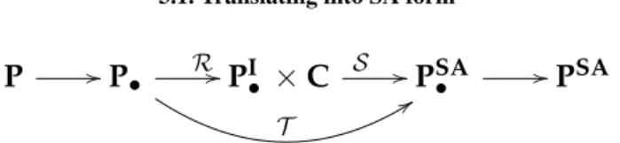
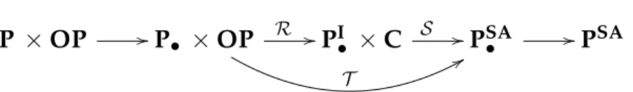
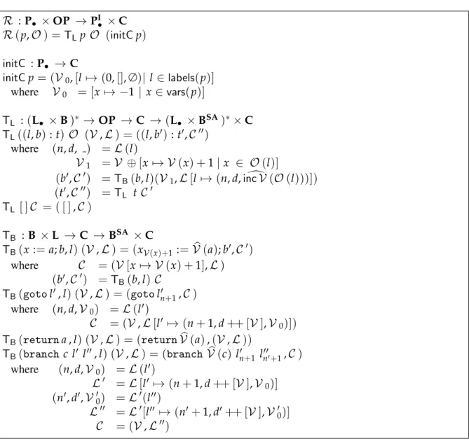
The translation fromP•into PSA• is performed by functionT and is done in two steps. In the first step we create an intermediate structure composed by a quasi SA program (SA program without φ-functions) -PI• = (L• ×BSA)∗ - and a context that registers information of the translation process. The second step uses this intermediate structure to add the φ-functions to the quasi SA program, producing a program inPSA• .The translation process is illustrated in Figure6. We name the first step R(after renaming) and the second stepS(after synchronization).
3.1. Translating into SA form
P //P• R // T
99
PI•
×
C S //PSA• //PSAFigure 6.: Translation into SA format
1. Converts the code of each block to SA form. This is done by tagging the variable with adequate indexes (versions);
2. Assigns a sequential number the incoming edge (or door) of each block.
TheSfunction is devoted to the synchronization task. Its only purpose is to build at the beginning of each block the assignments of φ-functions to the variables.
To implement the first step of the translation, we need to know:
• The current version of each variable. For that we need a function that maps each variable identifier to a non-negative integer. For a programp∈ P we let VSp =Varp →N whereVarp
denotes the set of variables of a programp. For the sake of simplicity, whenever it is clear what is the programp being translated, we drop the subscript p and write simply VS . We letV,V’, ... range overVS . We call version functions to the elements of VS .
Given a functionV = Var →N, we define the functionV =b Var → VarSA as being such that bV (x) = xV (x). bV is lifted toAexp and Cexp in the obvious way, renaming the variables according toV. Given a states and a versionV, bV (s)is the function bV (s) = VarSA →Z
that for allxi ∈VarSA, bV (xi) =s(x). For any labell, bV (l) =l.
Furthermore, given a version functionV ∈VS , we define an auxiliary function inc:: VS →VS
that increments the version of all the variables.
• The current number of edges arriving to a labeled block, i.e. , the number of already discovered doors of a labeled block, the version function associated to each door of a labeled block and the version of the variables to be synchronized. For a program p ∈ P we let LSp = Lp →
N×VS∗p×VSpwhereLpdenotes the set of labels of a programp. For the sake of simplicity,
whenever it is clear what is the programp being translated, we drop the subscript p and write simplyLS . We letL,L’, ... range overLS . We call label functions to the elements in LS .
We aggregate these informations in what we call a context. We letC = VS ×LS and letC,C’, ... range overC .
In the beginning of the translation, the context is initialized (by function initC ) and then incremen-tally built in the translation process, as we go through the given program inP•.
• The version function starts with all variables with version equal to−1. The versions are incre-mented at the beginning of each block, so the first version in use will be0;
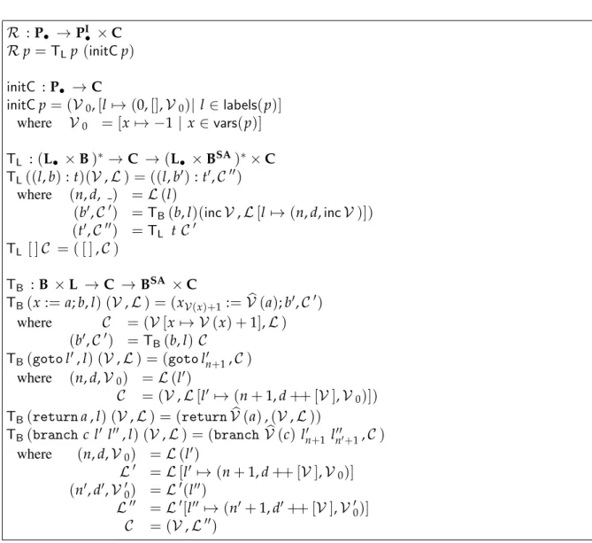
3.1. Translating into SA form R : P• →PI• ×C Rp=TLp (initCp) initC : P• →C initCp= (V0,[l7→ (0,[],V0)| l∈labels(p)] where V0 = [x7→ −1 |x ∈vars(p)] TL :(L• ×B)∗ →C → (L• ×BSA)∗×C TL((l, b): t)(V,L ) = ((l, b0): t0,C00) where (n, d, ) = L (l) (b0,C0) =TB(b, l)(incV,L [l7→ (n, d, incV )]) (t0,C00) =TL t C0 TL [ ] C = ( [ ],C ) TB : B ×L →C →BSA ×C TB(x := a; b, l) (V,L ) = (xV (x)+1:=V (b a); b0,C0) where C = (V [x7→ V (x) +1],L ) (b0,C0) =TB(b, l) C TB(gotol0, l) (V,L ) = (gotol0n+1,C ) where (n, d,V0) = L (l0) C = (V,L [l0 7→ (n+1, d++ [V ],V0)]) TB(returna , l) (V,L ) = (return bV (a),(V,L )) TB(branchc l0 l00, l) (V,L ) = (branch bV (c) l0n+1 l00n0+1,C ) where (n, d,V0) = L (l0) L0 = L [l0 7→ (n+1, d++ [V ],V0)] (n0, d0,V00) = L0(l00) L00 = L0[l00 7→ (n0+1, d0++ [V ],V00)] C = (V,L00)
Figure 7.: FunctionRand its auxiliary functions
• The label function begins with the labels with the respective number of discovered doors equal to0, an empty list of version functions and a version function which we assume to have−1 as-sociated to each variable (although the concrete number asas-sociated to each variable is irrelevant at this point).
The initC function uses auxiliary functions that we omit for the sake of simplicity (one can see the details in Appendix A). For a programp, vars(p)collects every variable of the program and labels(p)
collects every label of the program.
FunctionR, presented in Figure7, is defined using a mixture of mathematical notation and Haskell-like syntax. This function relies on two auxiliary functions: TLand TB. We give a brief description
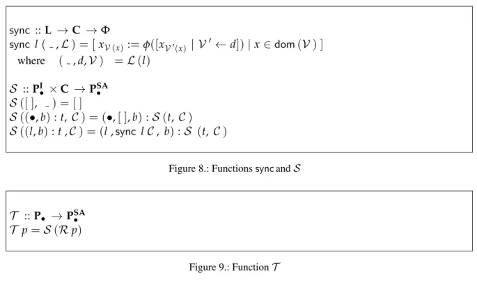
3.1. Translating into SA form sync :: L →C →Φ sync l( ,L ) = [ xV (x):=φ([xV0(x) | V 0 ← d]) |x∈dom(V ) ] where ( , d,V ) = L (l) S :: PI• ×C →PSA• S ([ ], ) = [ ] S ((•, b): t, C ) = (•,[ ], b):S (t, C ) S ((l, b): t ,C ) = (l , sync lC, b):S (t, C )
Figure 8.: Functions sync andS
T :: P• →PSA• T p= S (Rp)
Figure 9.: FunctionT
• TLiterates over the program, translating each block and carrying the corresponding auxiliary
context. It begins by incrementing the version of each variable, in order to spare a version for synchronization. This task is performed by the auxiliary function inc. The synchronization version of the block being translated is registered in the label function, by associating it to the label of the block.
• TBstarts the translation of a labeled block. TBreceives the block to be translated, its label and
the context. TBis responsible for:
(i) tagging the variables according to the version function and the SA format;
(ii) tagging the labels of the goto and branch commands according to the label function. Moreover, it updates the context coherently.
After we get the intermediate program (inPI•), it is necessary to synchronize the variables that can come from different doors. To do that, we must add the φ-functions. This operation is done by the functionS, which can be seen in Figure8. For the sake of simplicity, we assume that the φ-functions sequence follows some predefined order established over the set of variables (any order will do).
The final result of the translation into SA format is obtained by applying firstRand secondly apply the functionSas stated in Figure6,i.e. ,T = S ◦ R. We can see functionT in Figure9.
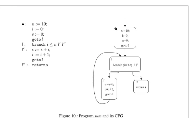
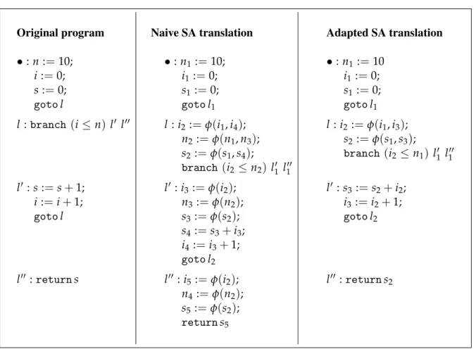
As it can be seen, this translation function synchronizes every variable of the program at the be-ginning of each block. This is obviously very inefficient and can be optimized. Using static analysis techniques it is possible to calculate the optimal placement of φ-functions that leads to a minimum
3.1. Translating into SA form
set of φ-functions. We did not follow that path because our focus is to prove the correctness of the translation with respect to the operational semantics, and we thought it was better to work with a naive version to begin with. However, we think this translation can be adapted to an optimized version if previously one calculates the optimal placement of the φ functions. With this information one would initialize the label function and, in the synchronization phase, the S function would only write the
φ-functions previously calculated. We will say more on this in Chapter8.
Let us now illustrate the translation done by function T with a small program. The following
GLprogram calculates the factorial of5.
Example 6 •: x :=5; f :=1; c :=1; gotol l : branchc≤x l0 l00 l0 : f := f∗c; c :=c+1; gotol l00: return f
We present the intermediate program and final context, after applying functionR.
•: x1 :=5; f1:=1; c1 :=1; gotol1 l : branch (c2 ≤x2)l10 l100 l0 : f4:= f3∗c3; c4 := c3+1; gotol2 l00 : return f5
3.1. Translating into SA form Final Context: Version Function:[(”c”, 5),(” f ”, 5),(”x”, 4)] Label Function: • (0,[],[(”c”, 0),(” f ”, 0),(”x”, 0)] ”l” (2,[[(”c”, 1),(” f ”, 1),(”x”, 1)],[(”c”, 4),(” f ”, 4),(”x”, 3)]],[(”c”, 2),(” f ”, 2),(”x”, 2)]) ”l0” (1,[[(”c”, 2),(” f ”, 2),(”x”, 2)]],[(”c”, 3),(” f ”, 3),(”x”, 3)]) ”l00” (1,[[(”c”, 2),(” f ”, 2),(”x”, 2)]],[(”c”, 5),(” f ”, 5),(”x”, 4)])
The SA version of the program after applying functionS, is the following:
•: x1 :=5; f1:=1; c1 :=1; gotol1 l : c2 := φ(c1, c4); f2:=φ(f1, f4); x2 :=φ(x1, x3); branch c2 ≤x2 l10 l100 l0 : c3 := φ(c2); f3:=φ(f2); x3 :=φ(x2); f4:= f3∗c3; c4 := c3+1; gotol2 l00 : c5 := φ(c2); f5:=φ(f2); x4 :=φ(x2); returnf5
We now show that T preserves the well-formedness of programs.
Proposition 3 Let p∈P•. If p is well formed thenT (p) is also well formed.
Proof.Assumep is a well-formed program in P•. We will now argue about the conditions defined in Definition9:
1. Each label is defined exactly once inT (p), sinceT does not change any name of label and each label was defined exactly one in p;
3.1. Translating into SA form
2. The numbering of the doors of each label is done sequentially, so each labelli invoked in a
goto or branch statement is unique inT (p);
3. Asp is well formed, each label invoked in p is declared so, sinceT does not change any label name,T (p) does not have undeclared labels;
4. As stated before, the numbering of the doors of each label is done sequentially, so if a labelliis
invoked in a goto or branch statement inT (p), so it is everyljwith0< j<i;
5. Inspecting the function sync displayed in Figure8we can see that the arity of φ-functions is equal to the number of edges recorded in the label function L, because the sync function is invoked with the context produced by Rafter processing all the program. Rconstructs coher-ently the context by starting with a context where the number of doors already found for each label is zero and updating this number each time a label is invoked and recording the version function associated to the recorded label;
6. By analyzing function TBdisplayed in Figure7 one can see that whenever there is an
assign-ment, the variable assigned receives the next index available for that variable and the version function is updated accordingly. This way, each variable SA will be assigned at most once in the block;
2 In the next chapter, we will show that functionT is correct, that is, that the translated program preserves the operational semantics of the original program.
4
C O R R E C T N E S S O F T H E T R A N S L AT I O N I N T O S A F O R M
In this chapter we prove that the translation of programs in GLto SA form, defined in the previous chapter, is correct relatively to the defined semantics, that is: the execution of a source program in
GLterminates with a certain result if and only if the execution of its translation into SA terminates with the same result. This will be established in Corollary 3, as a consequence of soundness and completeness results from the translationT (Theorem2and Theorem1)
To prove the correctness of the translation functionT , we separate each of the transition relations ;pdefined in the previous chapter, into two transition relations that will take into account whether
computation continues inside the block or jumps into another block.
In this chapter we will need the auxiliary function that follows. For p ∈ P•, b and b1 ∈ B, x ∈
vars(p)anda∈Aexp , the notation b=−−−−→(x := a); b1will mean that blockb comprises a sequence of
assignments−−−−→(x :=a), followed by blockb1. Also, forVa version function,V [
−−−−→
(x :=a)]will mean a new version functionV1such that:
V1( [ ] ) = V
V1(x :=a;−−−−−→(y := a1)) = V0[x 7→ V0(x) +1]
where
V0 = V1[−−−−→y :=a1]
This corresponds to the evolution of a version function in the process of translating a sequence of
GL-assignments in SA form.
Throughout this chapter we will assume that anyp∈ P• andp0 ∈ PSA• is well-formed.
4.1 S P L I T T I N G T H E T R A N S I T I O N R E L AT I O N O F T H E S O U R C E L A N G U A G E G L
4.1.1 Computation inside block
The new transition relation inG Linside blocks is given through a binary relation on configurations. The configurations are now triples hb, s,V i where b is a block, s is a state and V is a function that keeps the version of each variable. This will be important in the proofs latter in this chapter,
4.1. Splitting the transition relation of the source languageGL
since it allows the connection between execution of a program and execution of its translation into SA form. A terminal configuration inside a block has the form hd, s,V iford = r e t u r na , d =
g o t ol o r d = b r a n c h c l l0, i.e. , a terminal configuration is a configuration that represents jump or return instructions inside a block.
As this relation represents computation steps inside a block, the only rule that defines the relation has to do with assignments, as presented in the next definition.
Definition 13 (Transition relation for G Linside blocks) The transition relation inside blocks inG Lis denoted by →and is the binary relation on configurations given by the following rule:
hx := a ; b, s,V i → hb, s[x 7 → J a K(s) ],V [x 7 → V (x) +1] i
We represent by→∗the reflexive and transitive closure of→, that allows to put together a sequence of zero or more transitions. By→nwe representn transitions in the relation→.
Lemma 3 Let p ∈ P•. Letb1, b2 be two blocks. Lets1, s2 ∈ Σ. LetV 1,V 2 ∈ V S . We have,
for anyn ∈ N0:
hb1, s1,V 1i →n hb2, s2,V 2i =⇒ hb1, s1i;nphb2, s2i
Proof.Easy induction onn having in mind Definition13and Definition5(case atrib). 2
4.1.2 Computation across blocks
We define now the second transition relation to deal with the jump instructions. Here, the configura-tions are hc, s,V iforc := l or c = r e t u r na . Next, we present the definition of this relation in
G L. Before this, we will need an auxiliary function, vrs(l, p), that will produce the correct version of each variable to be used in the block labeled l in program p, which we define next.
Definition 14 (Synchronized versions) Let p ∈ P• and(l : b) ∈ p.
vrs(l , p) = [x 7 →i | xi ∈ dom(φ) a n d (l : φ b0) ∈ T (p) ]
Definition 15 (Transition relation across blocks inG L) Let p ∈ P• be a program in G L. The transition relation across blocks induced by p is a binary relation on configurations and is denoted
4.1. Splitting the transition relation of the source languageGL
by −◦→p, or simply−◦→, when it is clear the program we have in mind. This transition relation is defined by the following rules:
return (l : b) ∈ p hb, s,V i → ∗ hr e t u r na , s0,V 0i hl , s,V i −◦→p hr e t u r na , s0,V 0i goto (l : b) ∈ p hb, s,V i → ∗ h g o t ol0, s0,V 0i hl , s,V i −◦→p hl0, s0, vrs(l0, p) i branchT (l : b) ∈ p hb, s,V i →∗ hb r a n c h c l0 l0 0, s0,V 0i J c K(s 0) = T hl , s,V i −◦→p hl0, s0, vrs(l0, p) i branchF (l : b) ∈ p hb, s,V i →∗ hb r a n c h c l0 l0 0, s0,V 0i J c K(s 0) = F hl , s,V i −◦→p hl0 0, s0, vrs(l0 0, p) i
In a sequence of transitions across blocks, an intermediate configuration has the formhl, s,V iand a terminal configuration across blocks has the formhreturna , s0,V0i. We represent by−◦→∗
p the
reflexive and transitive closure of −◦→p, that allows to put together a sequence of zero or more
transitions. By−◦→n
pwe representn transitions on−◦→p.
Now we establish some basic results relating the transition relations; and−◦→forGLprograms. Lemma 4 Let p∈P• and(l : b1) ∈p. Let s1, s2 ∈Σ. We have one of the following, for some n:
1. hl, s1,V1i −◦→ hreturna , s2,V2i =⇒ hb1, s1i;nhreturna , s2i
2. hl, s1,V1i −◦→ hl0, s2,V2iimplies one of the following rules:
a) hb1, s1i;nhgotol0, s2i
or
b) hb1, s1i;nhbranchc l0 l00, s2iandJc K(s2) =T or
c) hb1, s1i;nhbranchc l00 l0, s2iandJc K(s2) =F
Proof.Follows easily from Definition15and Lemma3. 2
Lemma 5 Let p∈P• and(l : b1),(l0 : b2) ∈p. Let s1, s2∈ Σ. Let n=#
−−−−−→
(x :=e). We have that: 1. Ifb1 =
−−−−−→
(x :=e); return a andhb1, s1i;nhreturna , s2ithen,∀V1∃V2:
1.1. hb1, s1,V1i →n hreturna , s2,V2i
1.2. hl, s1,V1i −◦→ hreturna , s2,V2i
2. Ifb1 =
−−−−−→
4.1. Splitting the transition relation of the source languageGL
2.1. hb1, s1,V1i →n hgotol0, s2,V2i
2.2. hl, s1,V1i −◦→ hl0, s2, vrs(l0, p)i
3. Ifb1 =
−−−−−→
(x :=e); branch c l0 l00, andhb1, s1i;nhbranchc l0 l00, s2ithen,∀ V1∃ V2:
3.1. hb1, s1,V1i →n hbranch c l0 l00, s2,V2i
3.2. Depending on the meaning ofc , we have:
3.2.1. IfJc K(s2) =T ,hl, s1,V1i −◦→ hl0, s2, vrs(l0, p)i
3.2.2. IfJc K(s2) =F ,hl, s1,V1i −◦→ hl00, s2, vrs(l00, p)i
Proof. The parts1 are easy induction on n, and parts 2 follow then from the respective parts 1 and
Definition15. 2
Definition 16 (Execution of program p in a state s inGLw.r.t.−◦→) Let p be a program in P•. Let s ∈ Σ. The execution of the program p in the state s w.r.t.−◦→ is the sequence of transi-tions (using the transition relation−◦→) generated byh•, s,V1i, whereV1corresponds to the initial version function for translationT ,i.e. ,V1 =inc(π1(initCp)). When the execution is finite and has
terminal configurationhreturna , s1,V2i, we say that the result of the execution isJa K(s1)
Throughout this chapter, we assume that when we refer to the execution of aGL-programw.r.t. a state and we do not specify the relation, we refer to an executionw.r.t.;.
Let us prove that indeed the two semantics for aGL-program are equivalent. Proposition 4 Let p∈P• ands0∈ Σ.
1. If the execution of p in state s0 w.r.t.; is finite and has hreturna , sias terminal
configu-ration, then the execution of p in state s0 w.r.t.−◦→ is finite and has terminal configuration
hreturna , s,V ifor someV.
2. If the execution of p in state s0 w.r.t.−◦→ is finite and has hreturna , s,V i as terminal
configuration, then the execution ofp in state s0w.r.t.; is finite and has terminal configuration
hreturna , si.
Proof.Letb be the initial block of p so we have(•: b) ∈ p.
1. If the execution of p in state s0 with respect to the semantics of relation ; is finite and has
hreturna , sias terminal configuration, exists a finite sequence of jump instructions ji such
that hb, s0i;∗hj1, s1i;hbj1, s1i; ∗ hj 2, s2i;hbj2, s2i;· · ·; ∗ h returna , si
4.2. Splitting the transition relation in the SA language
wherejiare the goto or branch instructions in the execution of program p in state s0and each
bji is the block determined by the jumpjiand the statesi. So, by Lemma5, for someV,
h•, s0, π1(initCp)i −◦→ hl1, s1, vrs(l1, p)i −◦→ hl2, s2, vrs(l2, p)i −◦→ · · · −◦→∗ hreturna , s,V i
where theli are the labels determined by the corresponding jump instructionji and statesi. So,
there is a finite execution ofp in state s0w.r.t. the relation−◦→.
2. Conversely, if the execution of p in state s0w.r.t.−◦→ is finite and its terminal configuration
ishreturna , s,V i, then, using Lemma4, we can conclude that the execution of p in state s0
w.r.t.; has terminal configurationhreturna , si.
2
Corollary 1 Let p ∈ P• and s0 ∈ Σ. The execution of p in state s0 w.r.t. to ; is finite iff the
execution ofp in state s0w.r.t.−◦→is finite. Furthermore, when both executions are finite, the results
are the same.
Proof.Follows directly from Proposition4. 2
4.2 S P L I T T I N G T H E T R A N S I T I O N R E L AT I O N I N T H E S A L A N G U A G E
In the SA language, the relation; we defined in Chapter2will also be split in the same manner as for
GL, giving rise to a relation→for computations inside blocks and a relation−◦→for computations across blocks.
4.2.1 Computation inside blocks
The new transition relation inside blocks in SA is given through a binary relation on configurations. The configurations are now tripleshb0, s0,V iwhereb0 is a block in SA, s0 is a state SA and Vis a function that keeps the version of each variable. The transition relation inside blocks is similar to the transition relation inside blocks forGL-programs, which only has one rule related with assignments. Definition 17 (Transition relation for SA programs inside blocks) The transition relation inside blocks in SA programs is denoted by→and is the binary relation on configurations given by the following rule: hxi := a0; b0, s0,V i → hb0, s0[xi 7→Ja 0 K(s 0)] ,V [x7→ i]i
4.2. Splitting the transition relation in the SA language
Lemma 6 Let p0 ∈ PSA• . Letb10, b20 be two SA blocks and lets01, s20 ∈ ΣSA. LetV1,V2∈ VS . For
anyn∈N0, we have:
hb01, s01,V1i →nhb02, s02,V2i =⇒ hb01, s01i;nphb02, s02i
Proof.Easy induction onn having in mind Definition17and Definition10(case atrib). 2
As usual,→∗ represents the reflexive and transitive closure of→and→nrepresentsn transitions
between configurations of→.
4.2.2 Computation across blocks
We define the second transition relation to deal with the jump instructions for SA programs. The configurations are tripleshc0, s0,V iwherec0 = l or c0 = returna0, s0 is a SA state. We will need the function upd defined in Definition10and the following notion of synchronized versions applied to SA programs.
Definition 18 (Synchronized versions for SA programs) Letp0 ∈PSA• and letl be a label of p0. vrs(l, p0) = [x 7→i |xi ∈dom(φ)and (l : φb0) ∈ p0]
Definition 19 (Transition relation across blocks in SA) Let p0 ∈ PSA• . The transition relation in-duced byp0is a binary relation on configurations and is denoted by−◦→p0or simply−◦→when it is
clear the program we have in mind. This transition relation is defined by the following rules:
return (l : φb 0) ∈ p0 hb0, s0,V i →∗ h returna0, s00,V0i hl, s0,V i −◦→ p0 hreturna0, s00,V0i goto (l 0 : φ00b00), (l : φb0) ∈ p0 hb0, s0,V i →∗ hgotol0 i, s00,V 0i hl, s0,V i −◦→ p0 hl0, upd(φ00, i, s00), vrs(l0, p)i branchT (l0 : φ00b00), (l00: φ000b000), (l : φb0) ∈ p0 hb0, s0,V i →∗ hbranchc0 l0i lj00, s00,V0iJc0K(s00) =T hl, s0,V i −◦→ p0 hl0, upd(φ00, i, s00), vrs(l0, p0)i branchF (l0 : φ00b00), (l00: φ000b000), (l : φb0) ∈ p0 hb0, s0,V i →∗ hbranchc0 l0i lj00, s00,V0iJc0K(s00) =F hl, s0,V i −◦→ p0 hl00, upd(φ000, j, s00), vrs(l00, p0)i
It is important to recall that when the execution of a program consists of a jump into a block, an update of the state is required according to the correspondent φ-function.
4.2. Splitting the transition relation in the SA language
Definition 20 (Execution of program p0in a states0in SAw.r.t.−◦→) Letp∈ P• andp0 = T (p). Lets0 ∈ΣSA. Theexecution of the programp0 in the states0w.r.t.−◦→is the sequence of transitions (using the transition relation−◦→) generated byh•, s0,V1i, withV1 =inc(π1(initCp))
Firstly, we will see two lemmas relating the relations; and−◦→for SA programs.
Lemma 7 Let p0 ∈ PSA• ,(l : φb10),(l0 : φ0b0)and(l00 : φ00b00) ∈ p0. Lets01, s02∈ ΣSA. We have that,
for somen∈N0:
1. hl, s10,V1i −◦→ hreturna0, s02,V2i =⇒ hb01, s01i;nhreturna0, s0
2i
2. hl, s10,V1i −◦→ hl0, s02,V2iimplies one of the following: a) hb01, s10i;nhgotol0 i, s0iwheres02=upd(φ0, i, s0) or b) hb01, s10i;nhbranchc0 l0 i lj00, s0iandJc 0 K(s 0 2) =T wheres02=upd(φ0, i, s0) or c) hb01, s10i;nhbranchc0 l00 i l0j, s0iandJc 0 K(s 0 2) =F wheres02=upd(φ0, j, s0)
Proof.Follows easily from Definition19and Lemma6. 2
Lemma 8 Let p0 ∈ PSA• ,(l : φb10),(l0 : φ0b20) and (l00 : φ00b30) ∈ p0. Let s01, s02 ∈ ΣSA. Let
n=#−−−−−→(x :=e0). We have that:
1. Ifb10 =−−−−−→(x :=e0); return a0 andhb10, s01i;nhreturna0, s0
2ithen,∀V1∃V2:
1.1. hb01, s10,V1i →n hreturna0, s0
2,V2i
1.2. hl, s10,V1i −◦→ hreturna0, s02,V2i
2. Ifb10 =−−−−−→(x :=e); goto li0 andhb10, s01i;nhgotol0
i, s02ithen,∀V1∃V2:
2.1. hb01, s10,V1i →n hgotol0
i, s02,V2i
2.2. hl, s10,V1i −◦→ hl0, upd(φ0, i, s02), vrs(l0, p0)i
3. Ifb10 =−−−−−→(x :=e0); branch c0 li0 l00j , andhb01, s01i;nhbranchc0 l0
i l00j , s02ithen,∀V1∃V2:
3.1. hb01, s10,V1i →n hbranch c0 l0
i l00j , s20,V2i
3.2. Depending on the meaning ofc , we have:
3.2.1. IfJc0K(s02) =T ,hl, s01,V1i −◦→ hl0, upd(φ0, i, s20), vrs(l0, p0)i