REM WORKING PAPER SERIES
Financial Crises and Climate Change
João Tovar Jalles
REM Working Paper 0131-2020
May 2020
REM – Research in Economics and Mathematics
Rua Miguel Lúpi 20, 1249-078 Lisboa,
Portugal
ISSN 2184-108X
Any opinions expressed are those of the authors and not those of REM. Short, up to two paragraphs can be cited provided that full credit is given to the authors.
REM – Research in Economics and Mathematics Rua Miguel Lupi, 20
1249-078 LISBOA Portugal Telephone: +351 - 213 925 912 E-mail: [email protected] https://rem.rc.iseg.ulisboa.pt/ https://twitter.com/ResearchRem https://www.linkedin.com/company/researchrem/ https://www.facebook.com/researchrem/
1
Financial Crises and Climate Change
*
João Tovar Jalles
#May 2020
Abstract
We empirically assess by means of the local projection method, the impact of financial crises on climate change vulnerability and resilience. Using a new dataset covering 178 countries over the period 1995–2017, we observe that resilience to climate change shocks has been increasing and that advanced economies are the least vulnerable. Our econometric results suggest that financial crises (particularly systematic banking ones) tend to lead to a short-run deterioration in a country´s resilience to climate change. This effect is more pronounced in developing economies. In downturns, if an economy is hit by a financial crisis, climate change vulnerability increases. Results are robust to several sensitivity checks.
Keywords: climate change; vulnerability; resilience, local projection method, impulse response functions, recessions, financial crises
JEL codes: C23; C83; E30; G10; O30; Q40
* This work was supported by the FCT (Fundação para a Ciência e a Tecnologia) [grant numbers
UID/ECO/00436/2019 and UID/SOC/04521/2019]. The opinions expressed herein are those of the author and not necessarily those of his employers.
# ISEG – University of Lisbon. UECE – Research Unit on Complexity and Economics. Rua Miguel Lupi 20,
1249-078 Lisbon, Portugal. UECE is financially supported by FCT. Economics for Policy and Centre for Globalization and Governance, Nova School of Business and Economics, Rua da Holanda 1, 2775-405 Carcavelos, Portugal. Email:
2 1. Introduction
Climate change already poses a systemic risk to the global economy. The Global Financial Crisis reopened the debate on the compatibility between economic development and environmental protection but has also led to a wider discussion on the usefulness of environmental policies and actions within recovery packages.1 The current Covid19 pandemic, and the recession
that will follow, will do the same. In both these cases, the resulting fall in economic activity did lead to reductions in energy consumption and, thus, carbon dioxide - the major greenhouse gas - emissions.2 Indeed, carbon dioxide has been shown to fluctuate with economic situations and to
be highly (negatively) correlated with GDP and energy consumption (Gierdraitis et al., 2010; Lane, 2011; Stavytskyy et al., 2016).3 More importantly, in contrast with the oil price crises of the 1970s,
the last crisis did not lead to a structural change in the growth of emissions in the years that followed (Peters et al., 2011).4 Against this background, the Paris climate accord in 2015 – the
COP21 – was a landmark effort on the part of countries to set and monitor commitments to mitigate global warming and the effects of climate change.
For some authors, crises tend to lead to deferment and postponement of environmental projects and investments as surviving the crisis (and its subsequent recovery) becomes the aim, rather than becoming a “green” economy (Del Río and Labandeira, 2009). Others advocate the opposite, i.e., that crises provide an opportunity for developing and investing in low-carbon technologies that, in turn, could provide a way out of the downturn (Greenpeace, 2008). This paper aims to empirically test these two conflicting propositions and answer whether crises are environmentally friendly or not. A perusal of the literature reveals no such study.
Specifically, we empirically assess the impact of (financial) crises on climate change taking advantage of a new dataset of climate change vulnerability and resilience developed by the Notre
1 Given the lockdown observed in many countries as consequence of the Covid19 pandemic, polluting emissions have
been falling but many feel it will not fundamentally have a long-lasting impact on climate change.
https://www.bbc.com/future/article/20200326-covid-19-the-impact-of-coronavirus-on-the-environment
2 Several papers assessed the output-emissions decoupling hypothesis and how their cyclical relationship has changed
over time (see e.g. Cohen et al., 2018).
3 “The Panic of 1873” led to a global reduction of carbon dioxide emissions. The Great Depression of the 1930s led
to an even larger reduction of emissions. Siddiqi (2000), looking at the Asian Financial Crisis, defended some positive consequences stemming from it to the global environment.
4 This uncharacteristic bounce back in emissions can be attributed to: (1) the globally coordinated action of central
banks and initial fiscal stimulus; (2) the easing of energy prices reducing pressure for structural changes; (3) the continuing and accelerated increase in coal-fired power (IEA, 2013). In contrast, Dauvergne (1999) looking at the Asian Financial Crisis, concluded that it contributed to extensive environmental changes.
3
Dame Global Adaptation Institute (ND-GAIN). We use a sample of 178 advanced and developing economies between 1995-2017 and we rely on Jorda’s (2005) local projection method to trace the short to medium-term impact of crises on climate change. We find that financial crises (particularly systematic banking ones) tend to lead to a short-run deterioration in a country´s resilience to climate change. This effect is more pronounced in emerging market economies. In downturns, if an economy is hit by a financial crisis, climate change vulnerability increases.
2. Methodology
We estimate and trace out the average response of climate change indices in the aftermath of financial crises following the approach proposed by Jordà (2005).5 The first regression
specification takes the form:
𝑦𝑖,𝑡+𝑘− 𝑦𝑖,𝑡−1 = 𝛼𝑖 + 𝜇𝑡+ 𝛽𝑘𝐹𝐶𝑖,𝑡+ θX𝑖,𝑡+ 𝜀𝑖,𝑡 (1)
in which 𝑦𝑖,𝑡+𝑘 denotes a climate change index in country i in period t+k; 𝛼𝑖 are country fixed effects included to control for unobserved cross-country heterogeneity; 𝜇𝑡 are time effects to control to control for global shocks; 𝐹𝐶𝑖,𝑡 is our financial crisis dummy variable, which takes value 1 when a financial crisis took place and zero otherwise. 𝐹𝐶𝑖,𝑡 takes the value of 1 for the starting year of a given financial crises and 0 otherwise (to improve the identification and minimize reverse causality). X𝑖,𝑡 is a set of controls including two lags of the dependent variable, two lags of the
crisis variable and two lags of real GDP growth. 𝜀𝑖,𝑡 is an i.i.d. disturbance term satisfying standard
assumptions of zero mean and constant variance. Equation (1) is estimated via Ordinary Least Squares (OLS) for each k=0,..,7 with robust standard errors clustered at the country level. Impulse response functions (IRFs) are computed using the estimated coefficients 𝛽𝑘, and the confidence bands are obtained using the estimated standard errors of the coefficients 𝛽𝑘.
York (2012) elaborated on the nonlinear effects of polluting emissions to an increase in income during economic expansions and contractions. For this reason, in a second specification, the dynamic response is allowed to vary with the state of the economy6:
5 This approach has been advocated by Romer and Romer (2017), as a flexible alternative to vector autoregressions. 6 This is equivalent to the smooth transition autoregressive model developed by Granger and Terävistra (1993).
4 𝑦𝑖,𝑡+𝑘− 𝑦𝑖,𝑡−1 = 𝛼𝑖 + 𝜇𝑡+ 𝛽𝑘𝐿𝐹(𝑧𝑖,𝑡)𝐹𝐶𝑖,𝑡+𝛽𝑘𝐻(1 − 𝐹(𝑧𝑖,𝑡))𝐹𝐶𝑖,𝑡+ θ𝑀𝑖,𝑡 + 𝜀𝑖,𝑡 (2) with 𝐹(𝑧𝑖𝑡) = exp (−𝛾𝑧𝑖𝑡) 1+exp (−𝛾𝑧𝑖𝑡), 𝛾 > 0
in which 𝑧𝑖𝑡 is an indicator of the state of the economy normalized to have zero mean and unit variance. Despite substantial progress in methodologies to calculate potential output, there is still not a widely accepted approach (Borio, 2013). Mindful of the criticisms surrounding the use of the Hodrick-Prescott (HP) filter (such as the identification of spurious cycles - Cogley and Nason, 1995), the state of the economy is measured by the output gap computed via the recent Hamilton (2018) filter. Fit is a smooth transition function used to estimate the climate change impact of
financial crisis in expansions versus recessions. Auerbach and Gorodnichenko (2012) set 𝛾 = 1.5. Results do not qualitatively change for alternative positive values of 𝛾. M is the same set of control variables used in the baseline specification, but now including also two lags of 𝐹(𝑧𝑖,𝑡). Equation
(2) is also estimated using OLS.
3. Data
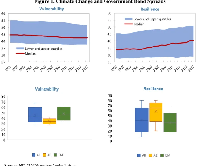
Our dependent variables are vulnerability and resilience to climate change as measured by the ND-GAIN indices, which capture a country’s overall susceptibility to climate-related disruptions and capacity to deal with the consequences of climate change, respectively.7 The composite indices are based on 45 indicators, of which 36 variables contributing to the vulnerability score and 9 variables constituting the resilience score. Vulnerability refers to “a country’s exposure, sensitivity, and capacity to adapt to the impacts of climate change”. Resilience, on the other hand, assesses “a country’s capacity to apply economic investments and convert them to adaptation actions”. Figure 1 shows the time profile and box-whisker plots for both the vulnerability and resilience indices. We observe that resilience to climate change shocks has been increasing, particularly since the early 2000s. From the bottom charts, we see that advanced economies are the least vulnerable (and more resilient) to climate change.
5
Financial crises come from Leaven and Valencia’s (2018) database which was recently updated, and which is publicly available. These include precise dating for (systemic) banking crises, currency crises, debt crises and sovereign debt restructurings. Real GDP is retrieved from the IMFs World Economic Outlook database.
4. Results
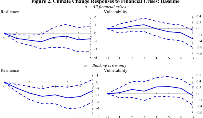
Figure 2 presents the results obtained by estimating equation (1). We observe that financial crises (irrespective of their type) tend to lead to a short-run deterioration in a country´s resilience to climate change (panel a). The resilience index falls by around 1 percent three years after the financial crisis (that is, two standard deviations). This suggests that financial crises negatively affect the ability to do climate friendly investments and/or take actions towards productive capacity
Figure 1. Climate Change and Government Bond Spreads
Source: ND-GAIN; authors' calculations. 25 30 35 40 45 50 55 60 Vulnerability
Lower and upper quartiles Median 25 30 35 40 45 50 55 60 Resilience
Lower and upper quartiles Median
6
adaptation/conversion. The main rationale is that crises, by making access to capital more difficult, negatively affect climate change mitigation efforts through their discouraging effects on investments (including those in low-carbon technologies) (Del Río and Labandeira, 2009). As both governments and the private sector focus on the recovery and on adapting their respective budgets, they shift priorities away from climate policies.8 The effect of crises on the vulnerability index is
not statistically different from zero throughout the horizon considered. In panel b. we see that the negative impact on climate change resilience is driven particularly by the negative effect coming from systemic banking crises (and to a lesser extent, debt crises – not shown).
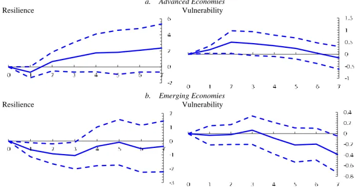
Splitting the sample between 34 advanced and 144 developing countries yields the IRFs in Figure 3. We see that developing economies are those more negatively affected in their resilience capacity by financial crises. In this group of countries, the stock of capital is smaller and, hence, their larger difficulties in adapting existing production structures to mitigate the impacts of climate
8 Our results do not support the findings of Sobrino and Monzon (2014) who looked at the environmental effects of
the Global Financial Crisis in Spain and found that it has led to higher energy efficiency on the road sector.
Figure 2. Climate Change Responses to Financial Crises: Baseline a. All financial crises
Resilience Vulnerability
b. Banking crisis only
Resilience Vulnerability
Note: blue continuous line denotes the impulse response from equation 1. Dotted blue lines are the 90 percent confidence bands. The horizontal axis is expressed in annual frequency. t=0 is the starting year of a financial crisis.
7
change. In the advanced economies subsample climate change vulnerability increases in the very short-run (up to two years after the crisis).
In Figure 4 we present the state-contingent results from estimating equation (2). In bad times, if an economy is hit by a financial crisis, climate change vulnerability increases, while resilience seems to be (statistically) unaffected. Depressed aggregate demand, the fall in the prices of some goods and lower economic capacity may encourage the consumption of goods with an inferior environmental quality (and lower prices) and to an over-exploitation of resources with associated environmental degradation (Del Río and Labandeira, 2009). Governments are also likely to avoid burdening business and industry with extra costs and regulation at a time when the economy is fragile and jobs may be at risk (Wooders and Runnalls, 2008).9 In recessionary times,
9 In fact, economic troubles ahead often prompt governments to loosen regulations. For instance, in the current
Covid19 pandemic, the US´ Environmental Protection Agency has cited the pandemic as justification for a decision to suspend enforcement of pollution rules. https://www.nationalgeographic.com/science/2020/04/pollution-made-the-pandemic-worse-but-lockdowns-clean-the-sky/
Figure 3. Climate Change Responses to Financial Crises: Advanced vs. Emerging Economies
a. Advanced Economies
Resilience Vulnerability
b. Emerging Economies
Resilience Vulnerability
Note: blue continuous line denotes the impulse response from equation 1. Dotted blue lines are the 90 percent confidence bands. The horizontal axis is expressed in annual frequency. t=0 is the starting year of a financial crisis.
8
carbon lock-in is also more likely as lower energy prices, reduce the economic viability for the development and operation of cleaner technologies. In good times, economies hit by a financial crisis see their vulnerability to climate change dropping continuously and persistently (becoming statistically significant in medium-run, that is, six years after the crisis).
We performed several sensitivity exercises. First, as shown by Tuelings and Zubanov (2010), a possible bias from estimating equation (1) using country-fixed effects is that the error term may have a non-zero expected value. This would lead to a bias of the estimates that is a function of k. Equation (1) was re-estimated by excluding country fixed effects. Results (not shown but available upon request) suggest that this bias is negligible. Second, equation (1) was re-estimated for different lags (l) of the control variables. Results (not shown but available upon request) confirm that previous findings are not lag-sensitive. Third, as an alternative variable measuring economic
Figure 4. Climate Change Responses to Financial Crises: The Role of Economic Conditions a. Resilience
Recession Expansion
b. Vulnerability
Recession Expansion
Note: blue continuous line denotes the impulse response from equation 2. Dotted blue lines are the 90 percent confidence bands. The yellow continuous line represents the unconditional baseline IRF from equation 1 (for comparison purposes). The horizontal axis is expressed in annual frequency. t=0 is the starting year of a financial crisis.
9
slack in equation (2), we also considered economic recessions identified using the Harding and Pagan (2002) algorithm to identify turning points. Results remained qualitatively unchanged.
5. Conclusion
We provided empirical evidence on the impact of financial crises on climate change for a sample of 178 countries between 1995-2017. We relied on the local projection method to plot impulse responses to find that crises (particularly banking ones) lead to a short-run fall in countries´ resilience to climate change (driven greatly by developing economies). In recessionary periods, an economy hit by a financial crisis, should expect is vulnerability to climate change to rise.
Econometric evidence presented here has clear policy implications, especially for developing countries that are relatively more vulnerable to risks associated with climate change. For policy makers, it is important so see financial crises as opportunities to make big reductions in emissions that one can then lock in, and ensure that energy pricing, investments and other policies are conducive toward innovations that create low-carbon societies. Although climate change is inevitable, the negative effect of crises on climate resilience shows that enhancing structural resilience through mitigation and adaptation, strengthening financial resilience through macroprudential preventive regulation and insurance schemes and improving economic diversification and policy management can help cope with the consequences of climate change for economic development.
10 References
Auerbach, A., Gorodnichenko, Y. (2012), “Fiscal Multipliers in Recession and Expansion.” In Fiscal Policy After the Financial Crisis, eds. Alberto Alesina and Francesco Giavazzi, NBER Books, National Bureau of Economic Research, Inc., Cambridge, Massachusetts.
Borio C., Disyatat P., Juselius M. (2013), “Rethinking Potential Output: Embedding Information about the Financial Cycle”, BIS Working Papers, n.404
Cogley, T., Nason, J. (1995), “Effects of the Hodrick-Prescott filter on trend and difference stationary time series Implications for business cycle research,” Journal of Economic Dynamics and Control, 19(1-2), 253- 278.
Cohen, G., Jalles, J., Marto, R., Loungani, P. (2018)” The Long-Run Decoupling of Emissions and Output: Evidence from the Largest Emitters”, Energy Policy, 118(c), 58-68
Dauvergne (1999)
Del Río, P., Labandeira, X. (2009), “Climate change at times of economic crisis”, FEDEA Coleccion Estudios Economicos, 05-09.
Gierdraitis, V., Girdenas, S., and Rovas, A. (2010), “Feeling the heat: Financial crises and their impact on global climate change”, Perspectives of Innovations, Economics and Business, 4(1), 7-10.
Granger, C., Teräsvirta, T. (1993), “Modelling Nonlinear Economic Relationships”. New York: Oxford University Press.
Greenpeace (2008), “Energy[r]evolution. A Sustainable EU-27 Energy Outlook”. Greenpeace International. November 2008.
Hamilton, J. (2018), “Why You Should Never Use the Hodrick-Prescott Filter,” Review of Economics and Statistics, 100(5), 831-843.
Harding, D., Pagan, A. (2002), “Dissecting the Cycle: A Methodological Investigation”. Journal of Monetary Economics, 49(2), 365-381.
Jordà, O. (2005), “Estimation and Inference of Impulse Responses by Local Projections.” American Economic Review 95 (1), 161–82.
Laeven, L., Valencia, F. (2018), “Systemic Banking Crises Revisited,” IMF Working Paper No. 18/206 Lane, J.-E. (2011), “CO2 emissions and GDP”. International Journal of Social Economics, 38, 911- 918. Peters, G. P., Marland, G., Le Quéré, C., Boden, T., Canadell, J. G., and Raupach, M. R. (2011), “Rapid growth in CO2 emissions after the 2008-2009 global financial crisis”. Nature Climate Change, 2(1), 2-4.
Romer, C. D., Romer, D. (2017), “New Evidence on the Aftermath of Financial Crises in Advanced Economies”, American Economic Review 107(10), 3072–3118.
Siddiqi, T. A. (2000), “The Asian Financial Crisis: is it good for the global environment?”, Environmental Change, 10, 1-7.
Stavytskyy, A., Giedraitis, V., Sakalauskas, D., and Huettinger, M. (2016), “Economic crises and emission of pollutants: a historical review of selected economies amid two economic recessions”, Ekonomia, 95(1).
Teulings, C., Zubanov, N. (2010), “Economic Recovery a Myth? Robust Estimation of Impulse Responses,” CEPR Discussion Paper 7300 (London: CEPR).
Wooders, P. Runnals, D. (2008), “The Financial Crisis and Our Response to Climate Change”. An IISD Commentary.
York, R. (2012), “Asymmetric effects of economic growth and decline on CO2 emissions”, Nature Climate Change. 2(11), 762-764.