Can we profit from natural disasters? : the role of catastrophe bonds

Can we profit from natural disasters?

The role of catastrophe bonds

Ana Filipa de Sousa Azevedo Simões

152412021

Abstract

We study the profitability of catastrophe bonds from January 2001 to June 2014. Our empirical analysis finds positive returns on catastrophe bonds and shows that they increase right after the Atlantic hurricane season and suffer a major downturn with the occurrence of significant catastrophes. Additionally, seasonality is found, especially during the month of September. When compared with stock and government bond benchmarks, returns on catastrophe bonds show considerably better results. However, when compared to the high yield bond benchmark, they present a similar performance. Finally, when tested for different predetermined variables, both traditional stock and bond market variables as well as liquidity risk do not explain catastrophe bond performance.

Professor José Faias Supervisor

Dissertation submitted in partial fulfillment of the requirements for the degree of International MSc in Finance, at Universidade Católica Portuguesa, February 2015

ACKNOWLEDGMENTS

Writing a master thesis was, without a doubt, the hardest thing I have had to do in all my academic life. The amount of information we gather in such short time is completely overwhelming, and requires a great extent of dedication and self-control in order to deal with all the problems we encounter when doing this work. During my research I found several challenges that I was only able to surpass with the help of some people that stood by my side in these hard moments.

Foremost, I would like to thank Professor José Faias, my thesis supervisor, for all the help and dedication he conceded to my thesis. He was the one who kept encouraging me to do better and never give up. He guided me in the moments I was lost and helped me every time I hit a dead end.

Further, I would also like to thank Swiss Re for their kindness in providing me the information I needed to develop this work; and both Fundação para a Ciência e Tecnologia (FCT) and Católica-Lisbon Research Unit for their financial support.

Additionally, I would like to dedicate this thesis to my good friends Filipa, Alex and Vitor. Their friendship and support were crucial while developing this work. All the stress, brainstorming and laughter we shared during this period made it seem much less difficult and much more gratifying. More importantly, I want to thank them for staying by my side in all the difficult moments and for being a part of my path at Católica.

Finally, I would like to show my sincere gratitude to my family. For all the patience they showed during this period and for believing that I could do great. I believe that it must have been difficult to deal with me during these stressful hard times.

The truth is that you have all contributed with inspiration to my personal and academic life, and without you, this thesis would not have been possible.

TABLE OF CONTENTS

1. Introduction ... 1

2. Background and cat bonds ... 4

3. Data ... 7

4. Empirical results ... 9

4.1. Cat bond returns and natural disasters ... 9

4.2. Monthly performance ... 13

4.3. Cat bonds and benchmarks ... 15

4.4. Market regressions and liquidity ... 19

5. Conclusion ... 30

LIST OF TABLES

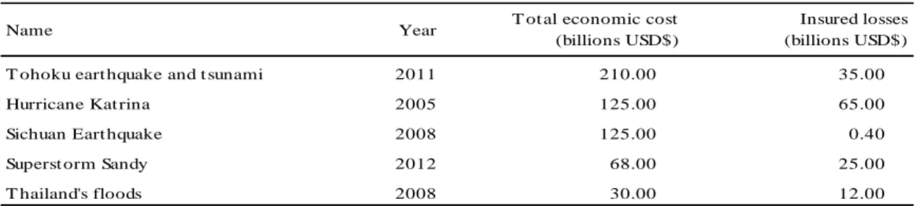
Table 1 –World’s five costliest disasters ... 4

Table 2 – Descriptive statistics of cat bonds ... 18

Table 3 – Explanatory regressions of cat bond returns over the risk free rate ... 23

Table 4 – Explanatory regressions of cat bond returns over LIBOR ... 27

LIST OF FIGURES Figure 1 – Cat bond returns ... 9

Figure 2 – Cat bond returns and events ... 11

Figure 3 – Cat bond average yield and events ... 13

Figure 4 – Cat bonds monthly performance ... 14

Figure 5 – Hurricane cat bonds monthly performance ... 15

1. Introduction

Past decades have shown significant costs arising from natural disasters. The huge concentration of property in catastrophe-prone areas has contributed to an increase in losses, making insurers skeptic when providing protection against catastrophe risk, which summed up with the growth in the number of policy holders, led to a shortage of capacity in the traditional reinsurance markets. Catastrophe bonds (“cat bonds”) were created as a way for insurance companies to transfer to investors’ part of their risks from natural disasters. Known for having low correlation with the stock market, cat bonds allow an increase in the investor’s portfolio diversification [Cummins (2008)].

A question we believe is of long-standing interest to academics and practitioners is whether cat bonds can be profitable. We ask, more specifically, whether the high risks associated with cat bonds are compensated by rewarding returns and whether there are ex ante variables that reliably explain these returns. To find that these securities are lucrative and that this could be explained through the use of common factors would complement modern investigation. Results illustrate that even though cat bonds are linked to high returns, pre-existing variables do not explain them.

Regardless of cat bond’s current growing importance, up until now, only a few number of researchers have shown interest on this subject. For example, Bantwal and Kunreuther (1999) focus on the reasons for the recent appeal of cat bonds and associate it with the attractive Sharpe ratios they uphold, despite their high uncertainty levels. Gurtler et al. (2014) find that right after the occurrence of natural disasters, the premiums on cat bonds increases. Additionally, they notice a dependence level between the cat bond market and the capital market right after the incidence of a natural disaster or financial crisis. Moreover, Ahrens et al. (2009) examine the impact of the hurricane season on cat bonds prices by analyzing if they have a different behavior than junk bonds when exposed to significant risk measures.

What this theme lacks is clearly specified evidence about the reaction of the cat bond market to large impact natural disasters. The relationship between financial crisis and this market is also quite unclear. Though some authors defend that there is no correlation between cat bonds and the financial market [see: Cummins (2008)], others state that a cat bonds’ performance is affected in the presence of a recessive economy. Hence, this thesis pursues two main objectives. First, we study cat bonds returns performance given the occurrence of a major natural disaster. Second, we investigate the relation of these securities with predetermined market variables in order to try to find any seasonality in unconditional expected returns. We also propose to analyze the impact of global financial crisis in cat bonds returns, as well as do a comparison with several benchmarks to test for similar performance.

We find that high impact events have a negative effect on cat bond’s prices. Moreover, the month of September is related with higher returns and, consequently, higher levels of volatility. Indeed, we find seasonality in cat bonds returns during the hurricane season that might suggest a tendency for higher risks around this period. Additionally, financial crises appear to have a very small impact on the prices of cat bonds, contrarily to what happens in the stock and bond market securities. This goes in line with other studies, such as Cummins (2008) and Bantwal and Kunreuther (1999) that defend the lack of correlation between the cat bond market and the capital stock market. We also find that the performance of cat bonds is similar to the one from junk bonds when excluding the period that corresponds to the 2008’s financial crisis, where returns of cat bonds show a better performance. However, a global financial crisis seems to both affect the capital market as well as the cat bond market, due to the increase in the level of risk aversion of potential investors.

In addition, we find that only a small number of variables have a significant explanatory power over returns and, thus, cannot be used to accurately explain them. Several studies have been developed with the purpose of finding factors capable of explaining returns of the stock and bond market, composing an extensive research on the subject [see: Gebhardt et al. (2005),

Fama and French (1993), Carhart (1997), Lin et al. (2011) and Keim and Stambaugh (1986)]. According to Lin et al. (2011), “financial theory suggests that expected asset returns are

related to systematic risk associated with common factors.” Also, the role of liquidity is often

important in determining whether an investment is viable or not. While several studies focus on the effect of this variable in the stock and bond market [see: Amihud (2002), Pástor and Stambaugh (2003), Sadka (2006) and Lin et al. (2011)], there are a very small, if any, number of studies that analyze the impact of liquidity in cat bonds. Hence, we run time-series regressions for cat bonds excess returns over the risk free rate estimation and over LIBOR, which include stock and bond market factors, as well as proxies for liquidity. Given the found seasonality in returns, we control for this effect while running regressions. Results improve when using excess returns over LIBOR, rather than when using excess returns over the monthly risk free rate estimation. Additionally, more variables show statistically significant results when using the LIBOR analysis.

Furthermore, given the high similarity in both assets, we compute a model regression using Merrill Lynch high yield bond index (“junk bonds”) and a dummy variable to control for the 2008’s crisis. Contrarily to what was observed with the previous models, results from this model are better when using the excess returns over the risk free rate instead of over LIBOR. In fact, all variables show a high explanatory power over cat bonds returns in the first analysis. However, this outcome is not linear through all indices and funds, showing a decreasing explanatory power when we narrow our analysis to specific disaster cat bonds (e.g. hurricane and earthquake cat bonds).

The remainder of this thesis is organized as follows. In Section 2, we document a number of facts about cat bonds, during the past decade. In Section 3, we identify the data used in our study and provide a multitude of descriptive statistics. In Section 4, we provide our results, where we analyze the behavior of returns when a major catastrophe occurs, search for

seasonality in performance and try to identify variables that can be used to explain returns. Finally, in Section 5, we draw our conclusions.

2. Background and cat bonds

In 1988, the Centre for Research on the Epidemiology of Disasters created the Emergency Events Database (“EM-DAT”), in order to provide the essential information on the occurrence and effects of the world’s mass disasters and thus, help in disaster alertness.1

Table 1 shows the world’s top five most expensive natural disasters between January 2001 and June 2014, including their corresponding economic costs and insured losses. In 2005, Hurricane Katrina became one of the deadliest and most expensive hurricanes in the history of US, reaching total economic costs of USD 125 billion and total insured losses of USD 65 billion.

Table 1 World’s five costliest disasters2

This table presents the world’s five costliest natural disasters between January 2001 and June 2014. We use the EM- DAT to access total economic costs and total insured losses of all natural disasters events. Data is sort from the world’s most to less expensive natural disaster.

However, the Tohoku earthquake and tsunami, that hit the coast of Japan in 2011, became the most costly natural disaster to ever occur, showing total economic damages of USD 210 billion and total insured losses of USD 35 billion. Moreover, in 2013 alone, total economic losses reached USD 140 billion (down from USD 196 billion in 2012), and global insured losses, from natural catastrophes and man-made disasters, a total of USD 45 billion (down from USD 81 billion in 2012).3

This said, cat bonds were issued and first used in the mid-nineties, after the occurrence of hurricane Andrew, in 1992, and Northridge earthquake, in 1994. They are part of a broader

1 _{See: http://www.emdat.be/database.}

2 _{Even though the Sichuan earthquake was considered one of the most expensive natural disasters of the past 10 years, with total estimated} costs of USD 125 billion, insurance costs were only USD 0.4 billion, the smallest from the group. This is due to the fact that rebuilding costs are cheaper in countries where the largest number of affected people is not covered by insurance

3_{Of this total value, USD 37 billion were generated from natural disasters and USD 8 billion from man-made claims (See:}

Name Year T ot al economic cost

(billions USD$)

Insured losses (billions USD$)

T ohoku eart hquake and t sunami 2011 210.00 35.00

Hurricane Kat rina 2005 125.00 65.00

Sichuan Eart hquake 2008 125.00 0.40

Superst orm Sandy 2012 68.00 25.00

class of assets known as insured-linked securities (“ILS”) and are related to the need of insurance companies to hedge their risk exposure when a major catastrophe occurs. In fact, cat bonds enable insurance companies to protect themselves from the possibility of natural disasters, by providing an alternative to traditional reinsurance. Thus, they became a standardized method of reallocating insurance risk from insurance companies to investors, who bear the risks of a specific catastrophe, within a particular time period, in exchange for attractive rates of investment.

So, how do catastrophe bonds work? Usually, a special purpose vehicle or insurer (“SPV” or “SPI”) enters into a reinsurance agreement with a sponsor for the issuance of cat bonds, in order to provide the necessary coverage. The sponsor receives the principal amount from investors and deposits it into a collateral account, typically investing in risk-free assets to generate money market returns. Thus, the coupons the investor receives are made from the interest the SPV or SPI receives from the collateral account and from the premiums the sponsor pays, which allow the bond to compensate with a significant high spread, typically between 8% to 15%.4 So, if a trigger event occurs, and the risk is materialized, then the investor forgoes all, or part, of its investment, which is liquidated by the SPV and used to reimburse the sponsor according to the terms of the contract. However, if no event happens, the cat bond behaves as a normal bond and the investor receives its payments until the term of the bond, as well as the bond’s principal at maturity.5 Typically, cat bond’s average maturity is between three to five years [Cummins (2008)]. Appendices A and B illustrate the previously described classical bond structure and provide an example of a cat bond’s standard characteristics. There are three types of trigger events that can cause a reduction in a cat bonds’ payment activity. The indemnity trigger is structured so that the actual loss is the one incurred by the issuer after the catastrophic event; the industry loss trigger is designed so that the actual losses of the issuer are aligned with the industry’s; and the parametric trigger is

4 _{See: http://www.schroders.com/globalassets/schroders/sites/pensions/pdfs/catastrophe-bonds-explained.pdf.} 5

structured so that the actual disaster characteristics (e.g. earthquake magnitude, tsunami height, etc.) are the ones used as a trigger.

Cat bonds have been attracting investors’ interest for being largely uncorrelated with the global market, which allows them to diversify their portfolio from more traditional asset classes, and, in extremely uncertain financial conditions, provides protection from market forces. In the supreme crisis of 2008, all assets prices faced a major decrease with the market uncertainty, including cat bonds. However, these securities were one of the few assets that presented positive returns in that year. Being known for carrying high levels of risk, cat bonds are, in their great majority, rated below investment grade bonds, meaning BB and B category ratings, making corporate high-yield bonds the most similar asset class. Nonetheless, since the first cat bond issuance, only ten cat bonds have defaulted, whereas when compared to other corporate bonds is actually a small number. The Tohoku earthquake was one of the last, and few, events where a cat bond, in fact, did default.

The market for cat bonds has been continuously increasing over the past years. In 2007 alone, the number of issued bonds reached a peak of USD 7.18 billion and the number of outstanding capital of USD 13.42 billion. Between 2007 and 2011, the market declined, at which point the increasing trend picked up again. At the end of 2013, total capital outstanding was worth USD 18.58 billion and issued capital was of USD 7.08 billion. Up until June 2014, total capital outstanding reached its all-time maximum with a total of USD 20.54 billion, worth of USD 5.701 billion in issued capital, which compared to single-handedly USD 250 billion in European corporate high-yield bonds makes it a quite small market [Swiss Re (2014)]. Still, the ILS investors’ base also picked up the increasing trend of the cat bond’s market. While ILS fund managers remain the largest group of investors, absorbing around 70% of new issuance, investor’s diversity has been growing as several institutional investors, money managers and pension funds, turn to this assets searching for a market with high returns and high liquidity profile. According to Aon Benfield Securities (2013), catastrophe

funds remain to be the main ILS investor, followed by institutional holders and mutual funds. In spite of the high spreads associated with cat bonds and the expansion of the market, this asset class still remains unavailable to smaller investors.

3. Data

Cat bonds can be structured to cover any type of natural disaster in any catastrophe-prone area. We examine monthly returns, from January 31st 2001 until June 30th 2014, for Swiss Re catastrophe bond indices, Aon Benfield ILS indices and LGT cat bond fund.

Swiss Re Capital Markets (“SRCM”) launched in 2007, the Swiss Re Cat Bond Performance Indices, to track down the returns of the cat bond market as a whole since 2002. They are a series of performance indices designed to track the price return and total rate of return of dollar denominated cat bonds and are updated on a weekly basis, on Friday, based on indicative prices provided by SRCM. Given the restricted basis of cat bonds investors, the investment weights of these indices are only available to those who have access to the SRCM weekly pricing indications. In this study, we choose to examine the Swiss Re Global Cat Bond Performance Index (“Swiss Re global index”), which represents the aggregate performance of all USD and EUR denominated cat bonds; and the Swiss Re US Wind Cat Bond Performance Index (“Swiss Re US wind index”) that tracks the total return for all USD denominated cat bonds exposed exclusively to US Atlantic Hurricane.

Moreover, the Aon Benfield ILS indices are computed by Thomson Reuters using month-end price data provided by Aon Benfield Securities. Aon Benfield Securities launched their indices three years after Swiss Re and they are base-weighted back to December 2000. Each index represents the total return an investor could achieve by allocating an amount of capital weighted to each cat bond available in the market in a particular period. We use the Aon Benfield All bond Index (“Aon all bond index”) that tracks the total rate of return for all outstanding catastrophe bonds; the Aon Benfield US Hurricane bond index (“Aon US hurricane index”) that tracks the total rate of return for all outstanding US hurricane, single

peril, catastrophe bonds; and the US Earthquake bond index (“Aon US earth index”) that incorporates the total rate of return for all outstanding US earthquake, single peril, catastrophe bonds. Both Swiss Re and Aon Benfield indices remain to be the only indices available that capture the performance inherent to cat bonds, with the single objective of improving the transparency of their returns, and thus allow them to be comparable to other financial assets. Finally, in this study, we incorporate a cat bond fund, due to the different characteristics it upholds when compared to cat bond indices. Contrarily to indices, funds are typically structured to incorporate management, subscription and performance fees, which reduce the performance of the bonds’ returns. The typical fee structure of cat funds ranges from a base of 1-2% of management fees and accumulates a performance fee that ranges between 10-15% [Risk Management Solutions (2012)]. The LGT (CH) Cat Bond Fund USD (“LGT cat bond fund”) is an open-end investment fund, incorporated in Switzerland, that invests in a broadly diversified portfolio of catastrophe bonds and whose final objective is a stable return above the money-market yield, with low correlation to the financial market. Contrarily to what was observed in the previous indices, this fund has a global focus. Moreover, total annual fees account for 8.75%, where a maximum of 5% is charged as a subscription fee, a maximum of 2% is charged as a redemption fee and the remaining 1.75% is charged as management fees. The fund requires a minimum investment of one unit and had an average of 59 positions on June 2014. Even though there are a great number of cat bond funds in the market with available information, the great majority only has information since 2009/2010. As such, and given the time-period analysis of our study, we choose to incorporate this fund, since it was the only one which dated back to 2001. The remaining data used in this work is described further as we use it in our analysis.

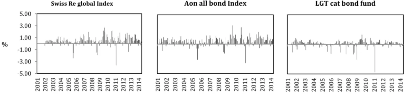
Figure 1 shows cat bonds excess returns. For simplification we present only our analysis for Swiss Re global index (left panel), Aon all bond index (middle panel) and LGT cat bond fund (right panel). The average monthly risk-free rate for this period is 0.14%. Returns show a

consistent pattern over time, although indicating some periods of high volatility where they take large negative jumps. Still, given the transaction costs associated with the fund, the LGT cat bond fund displays a more persistent performance than the two indices and, also, smaller returns.

Figure 1 Cat bond returns

This figure presents monthly excess returns for Swiss Re global index (left panel), Aon all bond index (middle panel) and LGT cat bond fund (right panel) from January 2001 to June 2014. The average monthly risk-free is 0.14%.

4. Empirical Results

The following section consists of several approaches using cat bond returns performance. Our basic objective is to ask whether cat bonds are related to positive returns and a profitable performance and whether these returns can be explained through the use of predetermined variables. In order to answer these questions we first study both the behavior of returns and yields during the occurrence of several high impact natural disasters as well as with the approximation of the hurricane season. Second, we investigate the monthly performance of both global cat bond indices and windstorm cat bond indices to search for any evidence of seasonality in returns. Third, we carry out an analysis to identify a similar pattern between cat bonds returns and the corporate market returns. Finally, we search for the explanatory power of multiple ex ante factors over these returns.

4.1. Cat bond returns and natural disasters

In order to understand the differences in returns, previously seen in Section 3, during the course of a year, and across the indices and fund, we investigate the impact of natural disasters on returns’ performances. Worldwide, tropical cyclone activity tends to be more

20 01 20 02 20 03 20 04 20 05 20 06 20 07 20 08 20 09 20 10 20 11 20 12 20 13 20 14

Aon all bond Index

-5.00 -3.00 -1.00 1.00 3.00 5.00 20 01 20 02 20 03 20 04 20 05 20 06 20 07 20 08 20 09 20 10 20 11 20 12 20 13 20 14 %

Swiss Re global Index

20 01 20 02 20 03 20 04 20 05 20 06 20 07 20 08 20 09 20 10 20 11 20 12 20 13 20 14

concentrated in late summer due to the differences in the temperature aloft and sea surface. There are two main hurricane seasons during a year: the Atlantic hurricane season, which runs from June 1st until November 30th, and typically peaks from late August to the end of September, and the Eastern Pacific hurricane season, which runs from May 15th until November 30th.6

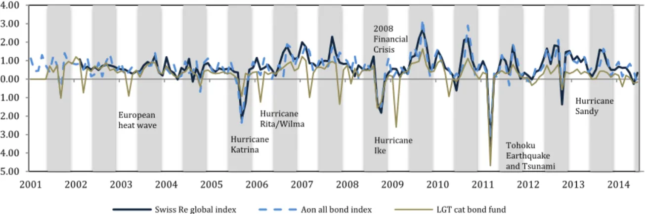
Figure 2 illustrates the behavior of returns for Swiss Re global index, Aon Benfield all bond index and LGT cat bond fund during the occurrence of natural catastrophes and with the approximation of the hurricane season. Given the areas of exposure of our cat bonds, we define as the hurricane season the period ranging between the months of June and November. In addition, we focus on the events that are historically known for having higher total estimated damages and a greater impact on market returns. We use EM-DAT to access the complete list of natural disasters and their respective total estimated damages.

Every year cat bonds suffer a major decrease during hurricane season. In 2005, the Atlantic hurricane season, that included three of the six most intense hurricanes, had a significant impact on bonds’ returns. From July to September, period corresponding to the appearance of hurricane Katrina, in August, and hurricanes Rita and Wilma, in September, returns decreased on average a total of 3 pp. However, when we narrow our focus to hurricane catastrophe bonds, returns do not suffer as much as previous ones. In fact, contrarily to what was expected, the average drop in hurricane bonds’ returns in this period is lower than the one verified before – Swiss Re US wind index registers a drop of 0.26 pp and Aon US hurricane index a drop of 2.37 pp. Thus, despite being considered one of the worst natural disasters in the US history in terms of insured losses, Hurricane Katrina had limited impact on hurricane cat bonds principal losses. This was due to the fact that the risks associated with these bonds were re-priced right after the incidence of Katrina, allowing returns to rise and, thus, offset the corresponding short-term losses.

-5.00 -4.00 -3.00 -2.00 -1.00 0.00 1.00 2.00 3.00 4.00 2001 2002 2003 2004 2005 2006 2007 2008 2009 2010 2011 2012 2013 2014 %

Swiss Re global index Aon all bond index LGT cat bond fund Hurricane Katrina Hurricane Sandy Hurricane Ike Hurricane Rita/Wilma 2008 Financial Crisis Tohoku Earthquake and Tsunami European heat wave

Figure 2 Cat bond returns and events

This figure shows the monthly returns of catastrophe bonds, given the occurrence of natural disasters, from January 2001 to June 2014. We choose the natural disasters that had a higher impact on the market. The shaded area represents the hurricane season defined from June until November.

The same situation materializes with the 2008’s hurricane season. The year of 2008 was particularly active in terms of hurricane manifestations, including sixteen named storms formed, of which five were major hurricanes, and over USD 47.5 billion in total damages. In September, hurricane Ike caused an average decrease of 2 pp on global returns and, contrarily to what was observed with hurricane Katrina, higher losses in hurricane bonds, which registered an average decrease of 4 pp. Additionally, the collapse of Lehman Brothers two days after the incidence of Hurricane Ike contributed to a difficult year for the ILS market. The bankruptcy of the well-known investment bank was the largest influencer on cat bonds market, causing a change in both cat bonds and typical bonds structures. No bonds were issued for the six months after the investment bank’s economic failure and, for the first time, the cat bond market lost its independence from the financial market.

However, the largest drop in returns happens in March 2011, marked by the appearance of the Tohoku’s earthquake and tsunami. The 2011’s Tohoku earthquake is known for being the most powerful earthquake ever recorded to have hit Japan and the fifth most powerful earthquake in the world’s history. Insured losses from the earthquake alone were between USD 14.5 billion and USD 34.6 billion and estimated total economic costs of USD 235 billion, making it the world’s most expensive natural disaster. Hence, total returns from cat bonds registered an average decrease of 4 pp from February to March and earthquake exposed

cat bonds a decrease of 1 pp. Despite the hard fall of returns in the aftermath of this powerful natural disaster, the market recovered strongly and was able to register a positive return for the full year – average return of 10%. The reason for this strong recovery is related to the fact that losses were mainly isolated on bonds exposed to Japan earthquake risk and so, had a small impact on US cat bonds.

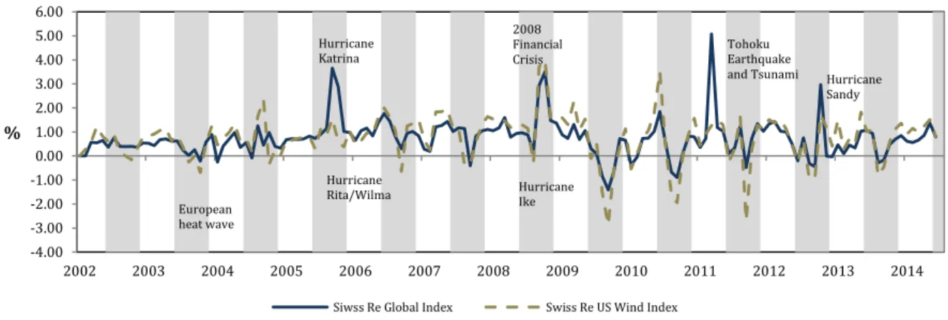
We present the same analysis for yields of cat bonds. Pricing of cat bonds depends on reinsurance prices and so, depends on the frequency and severity of natural disasters. As we saw, cat bonds’ prices tend to decrease in the aftermath of natural disasters, making yields of cat bonds rise and, thus, encouraging new issues to bring higher coupons to the market. Following the same reasoning, when a cat bond is in great demand – typically before the hurricane season, when prices on bonds are high – investors tend to pay more for the bond, and end up losing money, given that yields will be low or even negative. So, insurance companies typically issue cat bonds right after the occurrence of catastrophic events, when the price is down, in order to compensate for the loss in capital. This said, Figure 3 shows our analysis for the average annual yield of cat bonds following the occurrence of high impact natural disasters. Given the restricted amount of information in the market about the yields of cat bonds, we can only present Swiss Re global index and Swiss Re wind index in this analysis. Results show that fluctuations on yields and returns occur simultaneously, although, as expected, they behave in an opposite way. Hence, during the incidence of natural disasters yields typically increase. In October 2005, following the destructive hurricane season, yields rose from 1.16% to 3.65% for Swiss Re global index. Curiously, in the Swiss Re wind index, yields do not rose half as much, showing a more modest increase - from 0.3% to 1.55%. Nevertheless, as we progress throughout the years, the two indices yields tend to converge. With the 2008’s hurricane season, the variation on global cat bonds and wind bonds is quite similar, shifting from a negative yield of 0.29% to a remarkably positive yield of 3.7% for Swiss Re global index and 3.9% for Swiss Re wind index.

Figure 3 Cat bond average yield and events

This figure shows the annualized yield of catastrophe bonds, from January 2001 to June 2014. We present the natural disasters that had a higher impact on the market. Shaded area represents the hurricane season defined from June until November.

Once again, the biggest impact on the market is registered in March 2011, a consequence of Tohoku’s earthquake and tsunami. Following this calamity, yields changed more than 1000% - increasing from merely 0.4% to 5% -, from February to April.

4.2. Monthly performance

The results obtained in the previous section illustrate the existence of a cyclical pattern associated with cat bonds’ performance. Previous studies report evidence of several seasonal effects in assets returns like the January effect, the Monday effect, the Friday effect or the Sell

in May effect [see for example: Ritter (1988), Bouman and Jacobsen (2002), Schneeweiss and

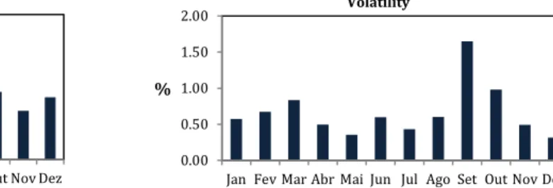
Woolridge (1979) and Keim (1983)]. Hence, we now focus our study on the monthly performance of cat bonds, with the purpose of trying to identify seasonality in cat bonds returns. In order to do this, we first compute the monthly mean and standard deviation of each index/fund and then we do a cross-sectional average of monthly returns and their respective volatility. Figure 4 shows the monthly performance of our catastrophe bonds. We find the same seasonality in returns as the one verified in previous studies. Returns are significantly larger between June and October and especially large in September (e.g. 1.10%). Moreover, volatility also shows a noteworthy increase during this month, which goes in line with the occurrence of the hurricane season.

-4.00 -3.00 -2.00 -1.00 0.00 1.00 2.00 3.00 4.00 5.00 6.00 2002 2003 2004 2005 2006 2007 2008 2009 2010 2011 2012 2013 2014 %

Siwss Re Global Index Swiss Re US Wind Index Hurricane Katrina Hurricane Sandy Hurricane Rita/Wilma 2008 Financial

Crisis Tohoku Earthquake and Tsunami

European heat wave

Hurricane Ike

0.00 0.50 1.00 1.50

Jan Fev Mar Abr Mai Jun Jul Ago Set Out Nov Dez

% Average 0.00 0.50 1.00 1.50 2.00

Jan Fev Mar Abr Mai Jun Jul Ago Set Out Nov Dez

%

Volatility Figure 4 Cat bonds monthly performance

This figure shows the monthly performance of catastrophe bonds. We compute the monthly mean and standard deviation of each index/fund and then we do a cross-sectional average of these statistics.

May, on the other hand, is the month where returns are smaller, showing an average return of 0.28%. Still, contrarily to what was verified in September, this is the second month where volatility is at its lowest (e.g. 0.35%), being December the first, with 0.32%. Given that the end of the Atlantic hurricane season is typically registered in the last days of November, returns decrease on average between the latter and May. The high percentage of hurricane cat bonds in total outstanding cat bonds – roughly 70% of all bonds - may be related to this evidence.

Previous results show a pattern in returns, where they achieve the highest value in September, which corresponds to the typical peak during the hurricane season. Thus, we now investigate whether average global returns behave this way due to the influence of hurricane cat bonds or, instead, all returns are swayed in this particular period. To do this, we replicate the previous analysis but now focus only on hurricane catastrophe bonds. Several hurricanes are known in the history of US for the mass destruction they caused as well as for the high values in damaged property they produced. For example, in August 23th 2005, the hurricane Katrina reached the coast of US and crossed southern Florida causing severe destruction along the Gulf coast. After destroying approximately a total of USD 125 billion in property, Katrina ended in August 31st 2005. Additionally, hurricane Sandy was formed on October 2012 in the western Caribbean Sea and became the second costliest hurricane in the history of US, affecting 24 US states, with particularly severe damage in New Jersey and New York. Total damages accounted for USD 68 billion, being USD 65 billion in US alone.

Figure 5 shows our results for this particular study. The differences in returns distribution is much more heightened on hurricane cat bonds than before. Still, September remains to be the month with the highest value of average returns and volatility – 1.93% and 1.95%, respectively. Furthermore, both the months of April and May show on average near zero returns, which did not happen in our previous analysis. Even so, when we narrow to hurricane cat bonds, volatility shows only a significant increase between August and October, remaining quite persistent in the other months.

Figure 5 Hurricane cat bonds monthly performance

This figure shows the monthly performance of hurricane catastrophe bonds. We compute the monthly mean and standard deviation of each index/fund and then we do a cross-sectional average of these statistics.

For each analysis, we do two hypothesis tests to check for the monthly equality between September returns and non-September returns and to check for the equality between September returns and all year’s average returns. The results obtained for the first analysis were for the non-rejection of the null hypothesis in both tests. However, for the second analysis, in the first test, only the months of June, August and October resulted in the non-rejection of the equality between the average of each month and the month of September. 4.3. Cat bonds and benchmarks

Usually, the approximation of the hurricane season creates a pressure for insurers to start issuing cat bonds, in order to cover the financial risks they will face with the upcoming disasters. Up until June 2014, total outstanding cat bonds hit a record level of USD 22 billion, allowing insurance companies to take advantage of the increasing search for a type of debt that offers high yields and has no correlation with the financial market. It is widely accepted in literature that cat bonds offer higher returns than the stock and bond market. As such, in this section, we present a comparison between cat bonds and three types of benchmarks, with

0.00 0.50 1.00 1.50 2.00 2.50

Jan Fev Mar Abr Mai Jun Jul Ago Set Out Nov Dez

% Average 0.00 0.50 1.00 1.50 2.00 2.50

Jan Fev Mar Abr Mai Jun Jul Ago Set Out Nov Dez

%

the objective of trying to identify the spread between cat bonds and several different assets. To do this, we use the S&P 500 index (“S&P500”), the 3-years Government bond index (“3y GB”) and the 3-years Merrill Lynch high-yield bond index (“junk bond”), all obtained from Bloomberg. Since the majority of the cat bonds included in the indices and funds are BB-rated - around 55% -, we choose to use a BB-rated high yield benchmark. High yield bonds or junk bonds are bonds that carry high probabilities of default and, thus, pay higher yields than normal fixed income. Yet, even though they present the same lack of correlation with the market as cat bonds, they carry higher probabilities of performing poorer than normal bonds when the equity market goes down.

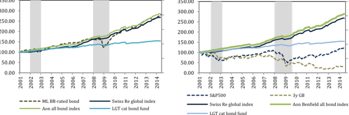
Figure 6 shows the comparison between cat bonds performance and the three different benchmarks. Given the high volatility associated with these assets, we choose to present cumulative returns for this analysis. On one hand, the right panel shows the comparison between S&P500, 3y GB and cat bonds cumulative returns. On the other hand, left panel presents the comparison between cat bonds and junk bonds cumulative returns.

Throughout the years, returns of all benchmarks have been decreasing, contrarily to what occurs with cat bonds, though presenting extremely high levels of volatility. When looking at the right panel, both S&P500 and 3y GB suffer with the occurrence of financial crises. The 2008 supreme crisis had a large impact on these securities, making their returns decrease by more than a half. The same, however, does not happen with cat bonds, which continue to increase despite both global economic recessions. Even though bearing high transaction costs, the cat bond fund also shows a tendency to rise, like the remaining cat bonds’ indices, yet showing a more persistent performance.

When we focus on the left panel, junk bonds show a similar performance to cat bonds than the other two benchmarks. However, as expected, and as we already saw with the other benchmarks, volatility is also higher in this index. During 2008’s financial crisis junk bonds cumulative returns decrease almost 70%. In fact, up until 2008, the spread between junk and

cat bonds was on average 0.13%, increasing to almost 9.73% during this period. So, returns of cat bonds became higher, between August 2008 and March 2010, than the ones from junk bonds. Again, the same impact did not happen with the cat bond fund, which performance only surpassed junk bonds between August 2008 and November 2008.

Figure 6 Cat bond returns and market benchmarks

This figure shows a comparison between cat bonds and three different benchmarks cumulative returns. Right panel shows the comparison between Swiss Re global index, Aon all bond index, LGT cat bond fund, S&P500 index and 3y GB index cumulative returns. Left panel presents the comparison between Swiss Re global index, Aon all bond index, LGT cat bond fund and junk bonds cumulative returns. Shaded area shows the occurrence of financial crises. We choose to present cumulative returns in order to eliminate the volatility noise associated with benchmarks.

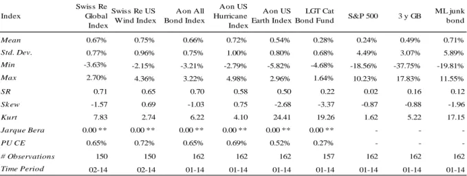
Additionally, descriptive statistics for catastrophe bonds and benchmarks are presented in Table 2. We compute all statistics using monthly returns. Sharpe ratio (“SR”) is computed by dividing the monthly’s excess return by its corresponding standard deviation. We use Fama-French monthly risk free rate in order to compute the monthly excess return. The average risk free rate for our study period is 0.14%.

Confirming what we previously observed, returns on cat bonds indices are higher than the ones from S&P500 and 3y GB, showing a positive average of 0.68%. Even returns for LGT cat bond fund, which are subject to high transaction costs, register a positive 0.28%.

Volatility, on the other hand, is also smaller for cat bonds. Even though hurricane bonds present a higher volatility than the rest of the cat bonds, it remains quite small when compared to the benchmarks. This said, and given the level of risk associated with cat bonds, returns are actually quite rewarding. This can be perceived trough the values of SR and Certainty Equivalent (“CE”). Even though Swiss Re and Aon Benfield indices show a higher SR than

0.00 50.00 100.00 150.00 200.00 250.00 300.00 350.00 20 01 20 02 20 03 20 04 20 05 20 06 20 07 20 08 20 09 20 10 20 11 20 12 20 13 20 14

ML BB-rated bond Swiss Re global index Aon all bond index LGT cat bond fund

0.00 50.00 100.00 150.00 200.00 250.00 300.00 350.00 20 01 20 02 20 03 20 04 20 05 20 06 20 07 20 08 20 09 20 10 20 11 20 12 20 13 20 14 S&P500 3y GB

Swiss Re global index Aon Benfield all bond index LGT cat bond fund

the cat bond fund, all cat bonds show a much better performance than the market, who’s SR are barely positive for S&P500 and slightly higher for 3y GB. As for the junk bond index, SR is quite similar to the one verified in the fund, although smaller than the rest of the sample. Moreover, a negative skewness is also present for the majority of the indices, with the exception of the two indices associated with the hurricane season (e.g. Swiss Re US wind index and Aon US hurricane index). This means that there is a higher probability for negative jumps in returns of these bonds, which can also be seen in Figure 1. Kurtosis, on the other hand, presents high values in our sample, especially for the earthquake cat bonds and for the fund. This may be explained by the fact that returns of cat bonds deviate strongly from the normal distribution, as we can see in Jarque Bera test. In fact, cat bonds usually provide a stable income, showing from time to time, when a major catastrophe occurs, large and unstable losses. This performance leads to heavy tails and a skewed distribution as we previously saw.

Table 2 Descriptive Statistics of cat bonds

This table presents descriptive summary statistics for catastrophe bonds, S&P 500, 3-years Government bonds and ML high-yield bonds monthly raw returns between January 2001 and June 2014. Mean is the mean return for each index monthly observations; Std. Dev. is the standard deviation of the indices monthly observations; Sharpe ratio and PU CE are respectively the Sharpe ratio and power utility certainty equivalent; Skew and Kurt measure respectively the skewness and kurtosis of the monthly observations; Jarque Bera represents the p-value obtained for the Jarque Bera test of returns. The symbol ** represents a rejection at a five percent significant level for returns following a normal distribution. We assume a relative risk aversion level of 5 to compute the certainty equivalent of the power utility function. Time period represents, in years, the period between the inception date of each index/fund until the end of our study period. The average risk free rate for our analysis period is 0.14%.

Additionally, we compute both Mean-Variance Certainty Equivalent and Power Utility Certainty Equivalent. In order to do this, we follow Brandt et. al (2009) and use a relative risk

Index Swiss Re Global Index Swiss Re US Wind Index Aon All Bond Index Aon US Hurricane Index Aon US Earth Index LGT Cat

Bond Fund S&P 500 3 y GB

ML junk bond Mean 0.67% 0.75% 0.66% 0.72% 0.54% 0.28% 0.24% 0.49% 0.71% Std. Dev. 0.77% 0.96% 0.75% 1.00% 0.80% 0.68% 4.49% 3.07% 5.89% Min -3.63% -2.15% -3.21% -2.79% -5.82% -4.68% -18.56% -37.75% -19.81% Max 2.70% 4.36% 3.22% 4.98% 2.96% 1.64% 10.23% 17.83% 11.55% SR 0.71 0.65 0.70 0.58 0.50 0.22 0.02 0.16 0.12 Sk ew -1.57 0.69 -1.03 0.75 -2.68 -3.37 -0.87 -0.88 -1.96 Kurt 7.83 2.74 6.22 4.10 24.41 19.26 1.62 5.22 17.15 Jarque Bera 0.00 ** 0.00 ** 0.00 ** 0.00 ** 0.00 ** 0.00 ** - - -PU CE 0.65% 0.72% 0.65% 0.69% 0.52% 0.27% - - -# Observations 150 150 162 162 162 157 162 162 162 Time Period 02-14 02-14 01-14 01-14 01-14 01-14 01-14 01-14 01-14

aversion level of five.7 For all bonds, CE decreases when the level of risk aversion increases and, again, statistics are higher in hurricane bonds. Further, when compared to the estimated risk free rate, CE is much higher, meaning that investors require rates of return greater than the risk free in order to bear the risk associated with natural disasters.

4.4. Market regressions and liquidity

In this section, we investigate whether a cat bonds expected return is positively related to market factors and liquidity risk. Previous studies show that there are several factors that have a strong explanatory power on corporate bonds returns. Thus, in this thesis we study whether these factors also explain cat bonds returns.

In 1993, Fama and French discover that both a term premium factor and a default premium factor capture most of the variation in returns of corporate and government bonds. Additionally, they find that when used alone the equity factors capture the majority of common deviation in bond returns, yet losing all explanatory power when the two-term structure factors are included. Elton et al. (2001) show that the change in corporate bonds spreads is related to systematic stock market factors. They incorporate Fama-French three factors in their regressions and find that the return in corporate bonds is related to both size and book-to-market factors. Lin et al. (2011) discover that liquidity risk has significant impact on corporate bond returns, even after controlling for the different stock and bond factors characteristics.

As such, in order to examine the impact of the stock and bond market, as well as liquidity risk, on cat bonds returns, we first specify a general model

r𝑡− rf𝑡=∝ + ∑ βj jfjt+ εt (1)

where r-rf is the monthly excess return during month t; βj is the sensitivity of changes in returns to factor j; and f is the return on factor j during month t.

7 _{Both statistics were computed using risk aversion levels of two, five and ten. However, given that results didn't diverge significantly as we} increased the level of risk aversion, we chose to only present our analysis for a risk aversion level of 5.

We divide this section as follows. First, we adapt Fama and French (1993) to our returns to try to identify if stock market returns can have an explanatory power on catastrophe bonds. We include in the previous methodology the momentum factor, formerly discussed by Carhart (1997), in order to capture momentum returns8

r𝑡− rf𝑡= α + β1. MKT + β2. SMB + β3. HML + β4. MOM + β5. SEP + ε (2)

where MKT is the stock market excess returns, SMB is the size factor, HML is the book-to-market factor and MOM is the momentum factor. We obtain all factors from K. French website and the sample period for these factors ranges between January 2001 and June 2014. Next, we include both a term and default premium factor, as proxies for the bond market returns

r𝑡− rf𝑡= α + β1. MKT + β2. SMB + β3. HML + β4. MOM + β5. TERM + β6. DEF + β7. SEP + ε (3)

where TERM is the term premium factor and DEF is the default premium factor. We obtain the term premium factor by subtracting the one-month Treasury bill return from the monthly long-term government bond return. Moreover, we obtain the default premium factor from the difference between the return on the market portfolio of long-term corporate bonds and the long-term government bond returns.

Finally, we follow Lin et al. (2011) by introducing three different liquidity measures

r𝑡− rf𝑡= α + β1. MKT + β2. SMB + β3. HML + β4. MOM + β5. TERM + β6. DEF + β7. L + β8. SEP + ε

where L is the liquidity factor, that can be either the Pástor-Stambaugh measure, the Amihud measure or the Sadka both permanent variable and transitory fixed variable. The Pástor-Stambaugh liquidity innovation measure focuses on temporary price changes related to the order flow [Pástor and Stambaugh (2003)]. Additionally, the Amihud illiquidity measure focuses on the price impact of trades and follows the idea that if liquidity is low, then a higher return should be expected, given a lower volume [Amihud (2002)]. Finally, Sadka (2006) identifies both a variable (informational) and a fixed (noninformational) component of price

impacts, induced by trades. We obtain all data from each author’s website.9 The sample period for Pástor-Stambaugh liquidity measure ends in December 2013 and Sadka’s liquidity components end in December 2010. In all equations we control for the previously observed returns seasonality (“September effect”), by using a dummy variable (“SEP”) that adopts the value 1 when in the presence of the month of September.

In its 2002 paper, Amihud describes liquidity as: “…an elusive concept. It is not observed

directly but rather has a number of aspects that cannot be captured in a single measure.”

Additionally, Lin et al. (2011) state that investors require higher profits on assets whose returns have greater sensitivities to marketwise liquidity. Hence, in this thesis we investigate whether cat bonds prices can be explained by several predetermined variables that reflect bond and stock prices as well as liquidity risk.

Given the similar results we obtained in Section 4.3. between the performance of cat bonds and junks bonds, we also construct a model regression using the junk bonds index (“ML”), previously discussed, and a dummy variable controlling for 2008’s financial crisis (“FC2008”).

r𝑡− rf𝑡= α + β1. ML + β2. FC2008 + ε

Therefore, we conduct time-series regression tests for all cat bonds monthly returns observations using these models. R2 is the R-squared statistic we achieve when computing each regression. The symbols ***, ** and * represent statistical significance at 1%, 5% and 10%, respectively.

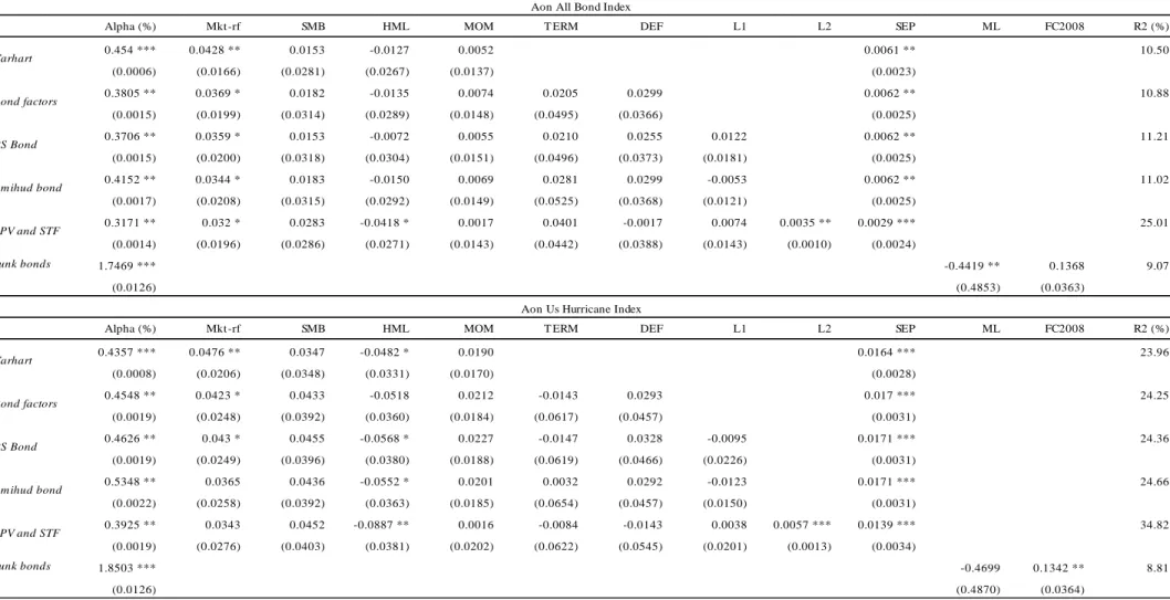
The results illustrated in Table 3 do not support the existence of statistically significant explanatory factors for cat bonds excess returns. As we increase the number of factors, alpha also increases, though showing modest changes. Moreover, the majority of these alphas are significantly different from zero, suggesting that the models are properly specified.

9 _{For Pástor-Stambaugh liquidity measure, see: http://faculty.chicagobooth.edu/lubos.pastor/research/. For Sadka’s liquidity components, see:} https://www2.bc.edu/ronnie-sadka/. For the Amihud liquidity measure I thank Maria Carolina Perry da Câmara for granting me access to this data.

The explanatory ability of these ex ante variables is seasonal, since the performance of the models is not half as strong when taking the SEP variable. Nevertheless, results show that expected excess returns are not significantly related to all betas, indicating that only three factors do a reasonably good job at explaining catastrophe bond returns – the market excess return, the September effect and Sadka’s liquidity measures. Additionally, they prove that contrarily to what was verified in the past with corporate bonds, both the term premium and the default premium are not significantly related to catastrophe bond’ excess returns. As for the poor performance of the remaining liquidity measures, this can be explained by the fact that both variables are not associated with bond returns, but instead with stock returns, given that the latter was not readily available. The R2 value of the regressions also increases as we change from one model to the other, having a significant change when we add the Sakda’s liquidity variables – ranging between 19.30 and 39.73. So, this strongly suggests that past discussed corporate bond factors do not show an explanatory power over cat bond returns and that liquidity risk is not an important factor for these bonds’ excess returns, when controlling for the September effect. As for our last model, using the junk bond index, it shows a strong explanatory power for global indices and both variables show a significance level either at 1% or 5%. However, when we narrow our model for specific cat bonds (e.g. hurricane and earthquake bonds), results lose their strength.

In the light of these findings, we finally conduct time-series regressions using cat bonds monthly excess returns over LIBOR. Cat bonds are known for providing high yields as compensation for the high risk they carry, usually related to a spread above LIBOR [Cummins 2008)]. Due to the high attractiveness of these securities, associated with the increase in diversification of portfolios, the spreads over LIBOR are typically low. Hence, we adapt the previously discussed models in order to introduce the LIBOR rate, instead of the risk free rate (Eq. 6).

Table 3 Explanatory regressions of cat bond returns over the risk free rate

This table shows coefficient estimations for Swiss Re global index, Swiss Re US wind index, LGT cat bond fund, Aon all bond index, Aon US Hurricane bond index and Aon US Earth bond index using Lin et. al (2011) methodology. We use French risk-free rate estimation to compute the excess return for all catastrophe bonds. The average estimation for the monthly risk-free rate is 0.14%. All regressions are computed using Fama-French’s four-factors. The term factor (TERM) is the monthly difference between the long-term government bond and the one-month T-bill rate. The default factor (DEF) is the monthly difference between the return of long-term investment grade bonds and the return of long-term government bonds. We use the Pástor-Stambaugh’s corporate bond liquidity factor, Amihud’s equity liquidity factor and Sadka’s permanent variable and transitory fixed stock market liquidity components as proxies for liquidity measures. We control for the September effect by using a dummy variable in our models that adopts the value one when in the presence of the month of September. R2 represents the R-squared statistic we obtain by computing each regression. Additionally, the ML factor is the Merrill Lynch high yield bond index. We also control for the 2008’s financial crisis by using a dummy variable that adopts the value one when in the presence of the financial crisis. Both alpha and R2 _{variables are presented in percentage. Brackets show the standard error for each coefficient. The symbols} ***, **, * show the significance level for 1%, 5% and 10% respectively.

Alpha (%) Mkt-rf SMB HML MOM T ERM DEF L1 L2 SEP ML FC2008 R2 (%)

0.4917 *** 0.042 ** -0.0077 -0.0082 -0.0007 0.0046 ** 7.49 (0.0007) (0.0169) (0.0286) (0.0272) (0.0140) (0.0023) 0.4812 ** 0.0388 * -0.0093 -0.0040 0.0003 -0.0005 0.0189 0.0045 * 7.45 (0.0016) (0.0203) (0.0321) (0.0295) (0.0151) (0.0505) (0.0374) (0.0025) 0.463 ** 0.0371 * -0.0144 0.0076 -0.0032 0.0003 0.0108 0.0223 0.0044 * 8.55 (0.0016) (0.0203) (0.0323) (0.0309) (0.0153) (0.0504) (0.0379) (0.0184) (0.0025) 0.5839 *** 0.0314 * -0.0088 -0.0084 -0.0012 0.0220 0.0188 -0.0157 0.0045 * 8.69 (0.0018) (0.0211) (0.0320) (0.0296) (0.0151) (0.0533) (0.0373) (0.0123) (0.0025) 0.4215 ** 0.0499 ** -0.0061 -0.0299 0.0105 0.0173 -0.0102 0.0296 ** 0.0021 ** 0.0012 19.30 (0.0014) (0.0196) (0.0285) (0.0270) (0.0143) (0.0440) (0.0386) (0.0142) (0.0010) (0.0024) Junk bonds 0.8144 *** -0.3661 *** 0.1453 * 10.29 (0.0133) (0.4986) (0.0369)

Alpha (%) Mkt-rf SMB HML MOM T ERM DEF L1 L2 SEP ML FC2008 R2 (%)

0.5159 *** 0.0524 ** -0.0152 -0.0214 0.0002 0.0111 *** 14.58 (0.0008) (0.0200) (0.0337) (0.0320) (0.0164) (0.0027) 0.6909 *** 0.0474 ** -0.0140 -0.0143 0.0029 -0.0647 0.0461 0.0112 *** 16.43 (0.0018) (0.0235) (0.0372) (0.0342) (0.0175) (0.0585) (0.0433) (0.0029) 0.6746 *** 0.0459 ** -0.0186 -0.0039 -0.0003 -0.0639 0.0388 0.0201 0.0111 *** 17.03 (0.0018) (0.0236) (0.0375) (0.0359) (0.0178) (0.0585) (0.0441) (0.0214) (0.0029) 0.795 *** 0.0399 * -0.0135 -0.0188 0.0014 -0.0419 0.0460 -0.0159 0.0112 *** 17.28 (0.0020) (0.0244) (0.0371) (0.0344) (0.0175) (0.0619) (0.0433) (0.0142) (0.0029) 0.6443 *** 0.0708 ** -0.0175 -0.0491 0.0104 -0.0588 -0.0102 0.0323 * 0.0026 ** 0.0064 ** 21.98 (0.0018) (0.0261) (0.0381) (0.0361) (0.0191) (0.0588) (0.0516) (0.0190) (0.0013) (0.0032) Junk bonds 0.9153 *** -0.3649 ** 0.1433 10.01 (0.0133) (0.4999) (0.0370)

Swiss Re US Wind Index

PS Bond

Am ihud bond

SPV and STF

Swiss Re Global Index

PS Bond Am ihud bond SPV and STF Carhart Bond factors Carhart Bond factors

Table 3 Explanatory regressions of cat bond returns over the risk free rate (continued)

This table shows coefficient estimations for Swiss Re global index, Swiss Re US wind index, LGT cat bond fund, Aon all bond index, Aon US Hurricane bond index and Aon US Earth bond index using Lin et. al (2011) methodology. We use French risk-free rate estimation to compute the excess return for all catastrophe bonds. The average estimation for the monthly risk-free rate is 0.14%. All regressions are computed using Fama-French’s four-factors. The term factor (TERM) is the monthly difference between the long-term government bond and the one-month T-bill rate. The default factor (DEF) is the monthly difference between the return of long-term investment grade bonds and the return of long-term government bonds. We use the Pástor-Stambaugh’s corporate bond liquidity factor, Amihud’s equity liquidity factor and Sadka’s permanent variable and transitory fixed stock market liquidity components as proxies for liquidity measures. We control for the September effect by using a dummy variable in our models that adopts the value one when in the presence of the month of September. R2 represents the R-squared statistic we obtain by computing each regression. Additionally, the ML factor is the Merrill Lynch high yield bond index. We also control for the 2008’s financial crisis by using a dummy variable that adopts the value one when in the presence of the financial crisis. Both alpha and R2 _{variables are presented in percentage. Brackets show the standard error for each coefficient. The symbols} ***, **, * show the significance level for 1%, 5% and 10% respectively

Alpha (%) Mkt-rf SMB HML MOM T ERM DEF L1 L2 SEP ML FC2008 R2 (%)

0.454 *** 0.0428 ** 0.0153 -0.0127 0.0052 0.0061 ** 10.50 (0.0006) (0.0166) (0.0281) (0.0267) (0.0137) (0.0023) 0.3805 ** 0.0369 * 0.0182 -0.0135 0.0074 0.0205 0.0299 0.0062 ** 10.88 (0.0015) (0.0199) (0.0314) (0.0289) (0.0148) (0.0495) (0.0366) (0.0025) 0.3706 ** 0.0359 * 0.0153 -0.0072 0.0055 0.0210 0.0255 0.0122 0.0062 ** 11.21 (0.0015) (0.0200) (0.0318) (0.0304) (0.0151) (0.0496) (0.0373) (0.0181) (0.0025) 0.4152 ** 0.0344 * 0.0183 -0.0150 0.0069 0.0281 0.0299 -0.0053 0.0062 ** 11.02 (0.0017) (0.0208) (0.0315) (0.0292) (0.0149) (0.0525) (0.0368) (0.0121) (0.0025) 0.3171 ** 0.032 * 0.0283 -0.0418 * 0.0017 0.0401 -0.0017 0.0074 0.0035 ** 0.0029 *** 25.01 (0.0014) (0.0196) (0.0286) (0.0271) (0.0143) (0.0442) (0.0388) (0.0143) (0.0010) (0.0024) Junk bonds 1.7469 *** -0.4419 ** 0.1368 9.07 (0.0126) (0.4853) (0.0363)

Alpha (%) Mkt-rf SMB HML MOM T ERM DEF L1 L2 SEP ML FC2008 R2 (%)

0.4357 *** 0.0476 ** 0.0347 -0.0482 * 0.0190 0.0164 *** 23.96 (0.0008) (0.0206) (0.0348) (0.0331) (0.0170) (0.0028) 0.4548 ** 0.0423 * 0.0433 -0.0518 0.0212 -0.0143 0.0293 0.017 *** 24.25 (0.0019) (0.0248) (0.0392) (0.0360) (0.0184) (0.0617) (0.0457) (0.0031) 0.4626 ** 0.043 * 0.0455 -0.0568 * 0.0227 -0.0147 0.0328 -0.0095 0.0171 *** 24.36 (0.0019) (0.0249) (0.0396) (0.0380) (0.0188) (0.0619) (0.0466) (0.0226) (0.0031) 0.5348 ** 0.0365 0.0436 -0.0552 * 0.0201 0.0032 0.0292 -0.0123 0.0171 *** 24.66 (0.0022) (0.0258) (0.0392) (0.0363) (0.0185) (0.0654) (0.0457) (0.0150) (0.0031) 0.3925 ** 0.0343 0.0452 -0.0887 ** 0.0016 -0.0084 -0.0143 0.0038 0.0057 *** 0.0139 *** 34.82 (0.0019) (0.0276) (0.0403) (0.0381) (0.0202) (0.0622) (0.0545) (0.0201) (0.0013) (0.0034) Junk bonds 1.8503 *** -0.4699 0.1342 ** 8.81 (0.0126) (0.4870) (0.0364) PS Bond Am ihud bond SPV and STF Carhart Bond factors

Aon All Bond Index

Am ihud bond

SPV and STF

Aon Us Hurricane Index

Carhart

Bond factors

Table 3 Explanatory regressions of cat bond returns over the risk free rate (continued)

This table shows coefficient estimations for Swiss Re global index, Swiss Re US wind index, LGT cat bond fund, Aon all bond index, Aon US Hurricane bond index and Aon US Earth bond index using Lin et. al (2011) methodology. We use French risk-free rate estimation to compute the excess return for all catastrophe bonds. The average estimation for the monthly risk-free rate is 0.14%. All regressions are computed using Fama-French’s four-factors. The term factor (TERM) is the monthly difference between the long-term government bond and the one-month T-bill rate. The default factor (DEF) is the monthly difference between the return of long-term investment grade bonds and the return of long-term government bonds. We use the Pástor-Stambaugh’s corporate bond liquidity factor, Amihud’s equity liquidity factor and Sadka’s permanent variable and transitory fixed stock market liquidity components as proxies for liquidity measures. We control for the September effect by using a dummy variable in our models that adopts the value one when in the presence of the month of September. R2 represents the R-squared statistic we obtain by computing each regression. Additionally, the ML factor is the Merrill Lynch high yield bond index. We also control for the 2008’s financial crisis by using a dummy variable that adopts the value one when in the presence of the financial crisis. Both alpha and R2 _{variables are presented in percentage. Brackets show the standard error for each coefficient. The symbols} ***, **, * show the significance level for 1%, 5% and 10% respectively

Alpha (%) Mkt-rf SMB HML MOM T ERM DEF L1 L2 SEP ML FC2008 R2 (%)

0.3892 *** 0.0449 ** -0.0035 -0.0582 ** 0.0131 -0.0018 8.31 (0.0006) (0.0161) (0.0271) (0.0258) (0.0132) (0.0022) 0.3967 ** 0.0253 -0.0047 -0.0576 ** 0.0185 -0.0024 0.0981 ** -0.0012 14.28 (0.0014) (0.0188) (0.0297) (0.0273) (0.0140) (0.0467) (0.0346) (0.0024) 0.4004 ** 0.0257 -0.0036 -0.06 ** 0.0193 -0.0026 0.0998 ** -0.0045 -0.0012 14.33 (0.0015) (0.0189) (0.0300) (0.0288) (0.0143) (0.0469) (0.0353) (0.0171) (0.0024) 0.4192 ** 0.0237 -0.0046 -0.0586 ** 0.0182 0.0025 0.0981 ** -0.0034 -0.0012 14.34 (0.0016) (0.0196) (0.0298) (0.0276) (0.0140) (0.0496) (0.0347) (0.0114) (0.0024) 0.415 ** 0.0151 -0.0098 -0.0853 *** 0.0013 -0.0148 0.0852 ** -0.0021 0.0052 *** -0.0042 * 39.73 (0.0014) (0.0196) (0.0285) (0.0270) (0.0143) (0.0440) (0.0386) (0.0142) (0.0010) (0.0024) Junk bonds 1.6423 *** -0.4819 0.1375 9.14 (0.0127) (0.4888) (0.0365)

Alpha (%) Mkt-rf SMB HML MOM T ERM DEF L1 L2 SEP ML FC2008 R2 (%)

0.0988 0.0305 ** -0.0119 0.0320 -0.0056 0.0028 7.45 (0.0006) (0.0149) (0.0251) (0.0239) (0.0123) (0.0020) -0.0321 0.0263 * -0.0207 0.0354 -0.0012 0.0480 0.0412 0.0032 10.00 (0.0014) (0.0179) (0.0283) (0.0260) (0.0133) (0.0445) (0.0330) (0.0022) -0.0315 0.0264 * -0.0206 0.0350 -0.0011 0.0480 0.0415 -0.0008 0.0032 10.01 (0.0014) (0.0180) (0.0286) (0.0274) (0.0136) (0.0447) (0.0336) (0.0163) (0.0022) -0.0693 0.029 * -0.0209 0.0370 -0.0007 0.0399 0.0412 0.0057 0.0032 10.21 (0.0016) (0.0187) (0.0283) (0.0262) (0.0134) (0.0472) (0.0330) (0.0108) (0.0022) -0.0646 0.0288 * -0.0087 0.0265 0.0052 0.0669 * 0.0471 0.0042 0.0011 0.0016 19.94 (0.0012) (0.0172) (0.0250) (0.0237) (0.0125) (0.0386) (0.0339) (0.0125) (0.0008) (0.0021) Junk bonds 1.0903 *** -0.5184 ** 0.1393 * 9.68 (0.0128) (0.4915) (0.0366) SPV and STF PS Bond Am ihud bond SPV and STF Carhart Bond factors Carhart Bond factors

Aon US Earth Index

LGT Cat Bond Fund

PS Bond

Table 4 reports the results for the adapted time-series regressions. We use the one-month LIBOR, extracted from Bloomberg, to compute the monthly catastrophe bond returns above LIBOR.

The results obtained when implementing equation 6 are much better than previous ones. Contrarily to what was observed before, the majority of liquidity betas are significant at a 1% and 5% levels and both the default premium factor and the momentum factor show significance at a 5% and 10% level, respectively, for almost all bonds. Thus, we can conclude that five out of eight factors have a significant impact on cat bonds excess returns over the one-month LIBOR. Also, size and term premium are the variables demonstrating the worst results for our models. As for the dummy variable, controlling for the September effect, it presents completely opposite results from before, showing no explanatory power. Moreover, the intercepts display a better performance with this model, yet not showing, in their great majority, any significance level, with the exception of the alpha obtained when using the Carhart model.

Nonetheless, the R2 statistic presents now higher values, though still showing the same behavior as before, meaning it tends to increase as we pass from one model to the other, presenting the highest value when we use Sadka’s liquidity measure – now with results ranging from 46.65 to 48.16. Curiously, when we compute Eq. 5, results are worse when we subtract LIBOR than when we subtract the risk free rate. In all bonds, both alpha and junk bonds show no significance. Additionally, the model presents no explanatory power over cat bonds returns. Overall, results strongly suggest that expected cat bonds excess returns over LIBOR are affected by betas of market risk, default premium and liquidity factors.