Classification of new electricity customers based on
surveys and smart metering data
Joaquim L. Viegasa,∗, Susana M. Vieiraa, R. Mel´ıcioa,b, V. M. F. Mendesb,c, Jo˜ao M. C. Sousaa
aIDMEC, LAETA, Instituto Superior T´ecnico, Universidade de Lisboa,
Av. Rovisco Pais, 1, 1049-001 Lisbon, Portugal
bDep.de F´ısica, Escola de Ciˆencias e Tecnologia, Universidade de ´Evora, Portugal cInstituto Superior de Engenharia de Lisboa
Abstract
This paper proposes a process for the classification of new residential elec-tricity customers. The current state of the art is extended by using a combi-nation of smart metering and survey data and by using model-based feature selection for the classification task. Firstly, the normalized representative consumption profiles of the population are derived through the clustering of data from households. Secondly, new customers are classified using survey data and a limited amount of smart metering data. Thirdly, regression anal-ysis and model-based feature selection results explain the importance of the variables and which are the drivers of different consumption profiles, enabling the extraction of appropriate models. The results of a case study show that the use of survey data significantly increases accuracy of the classification task (up to 20%). Considering four consumption groups, more than half of the customers are correctly classified with only one week of metering data, with more weeks the accuracy is significantly improved. The use of model-based feature selection resulted in the use of a significantly lower number of features allowing an easy interpretation of the derived models.
Keywords:
Data-driven energy efficiency, Electricity customer clustering, Classification of new residential customers, Customer feature selection, Smart metering data, Customer surveys data
∗Corresponding author.
1. Introduction 1
A game-changing shift has been happening in the utility industry and 2
energy markets. Policy focused on energy efficiency and sustainability is 3
growing fruit of the awareness of current environmental challenges. Liber-4
alization, growing competition between utilities, technological advancements 5
and policy towards a sustainable use of energy sources are pushing utilities 6
to seek innovation and new market related insights. 7
Electricity is a main energy carrier used around the world for supporting 8
the primary, secondary and tertiary sectors. The commercial and residential 9
energy demand is expected to continue to shift towards electricity and away 10
from primary fuels. By 2040, forecasts indicate that electricity generation 11
will account for more than 40% of global energy consumption and, from 2010 12
to 2040, global electricity demand is projected to increase by about 85% [1–3]. 13
Technological advancement in the fields of metering, communications and 14
computation are enabling utilities to monitor and save huge amounts of data 15
related to their operation. The deployment of electricity meters with two-16
way communication capabilities is enabling the logging of the consumption of 17
users with high resolution. The number of advanced metering infrastructure 18
(AMI) installations, also known as smart meters, has surpassed the number 19
of traditional one-way communication meters in the United States [4]. Close 20
to 45 million smart meters are already installed in three Member States 21
(Finland, Italy and Sweden) of the European Union (EU), representing 23 22
percent of the envisaged installation in the EU by 2020 [5]. 23
The consumption data of customers has the potential to give insights of 24
great importance for utilities and policy makers. Valuable insights can be 25
derived by the knowledge of typical consumption curves of different consumer 26
groups and understanding what are the main drivers of consumption. This 27
knowledge can assist decision makers in the electricity utility industry in de-28
veloping demand side management (DSM) programs, consumer engagement 29
strategy, marketing, alternative tariff setting methods and demand forecast-30
ing tools [6]. Knowledge on the way different demographic groups consume 31
electricity is valuable to study the effect of energy policy on different popu-32
lation groups. 33
The high number of consumers and desired high sampling frequencies in 34
smart metering implies that huge amounts of data have to be stored and 35
processing grows in complexity. Computational intelligence techniques in
36
the fields of machine learning are starting to be extensively used in order
to extract knowledge from the data coming from the grid. These techniques
38
can provide decision makers with predictive models and the ability to extract
39
valuable knowledge.
40
In order to characterize the behaviour of electricity customers, the clus-41
tering of electricity consumption data has been the focus of a considerable 42
amount of research in the past years. The usual stated applications range 43
from the design and simulation of DSM [7, 8], load forecasting [9–11], tariff 44
setting [12–14], marketing and bad data detection. The clustering meth-45
ods found to be used are mostly the K-means algorithm [8, 15–18]. Fuzzy 46
clustering [19] has shown promise in the field. Data preparation is of high 47
importance in these applications, dictating what information is desired to be 48
extracted from the clustering and the ability of the used methods to achieve 49
good results. Normalization, parametric modelling [10], temperature based 50
normalization [16, 20] and wavelet transformation [9] have been found to be 51
used in the literature. 52
The use of static data related to household characteristics, e.g., income, 53
number of inhabitants, education, construction year and appliances in rela-54
tion to static or dynamic energy consumption data is being studied in order 55
to find the main drivers of residential energy consumption. In [21–23] fac-56
tor analysis and linear regression are used to find the main determinants of 57
energy consumption in residential settings, such as weather data, household 58
characteristics and demographics. In [24] demographic data and psychologi-59
cal and belief related data is studied in comparison to energy consumption. 60
[25, 26] presents studies on the prediction of household information based 61
on smart meter data. In [27, 28] consumptions profiles obtained via clus-62
tering are correlated to household characteristics. In [29] a methodology 63
is presented for the characterization of medium voltage electricity customers 64
through clustering and posterior modelling for which the classification of new 65
customers is stated as a possible application. 66
Classifying new customers is crucial for marketing purposes, as customers 67
with lengthy relationships are less likely to defect and are less affected by new 68
information and offers. Thus, a greater impact of marketing strategies and 69
engagement is expected with new customers [30, 31]. 70
This paper extends the current state of the art by developing a process 71
for the classification of new electricity customers using not only metering 72
data but also using static data on household characteristics. The use of a 73
limited amount of metering data is done in order to emulate the analysis of 74
new electricity customers for which only a small amount of data is available. 75
The use of model-based feature selection for the discovery of the consumption 76
drivers shows promise in the field. 77
Based on the clustering of customers’ electricity consumption data, the 78
consumption profile of new customers is predicted using survey data and 79
a limited amount of smart metering data. Classification models in combi-80
nation with model-based and filter feature selection are compared for the 81
classification task, selection and analysis of variables. 82
The developed process aims to provide an interpretable classification 83
modelling method for the classification of electricity customers and discovery 84
of the drivers of different electricity consumption profiles. The presented
re-85
sults aim to illustrate the application of the proposed process, using data that
86
resulted from smart metering trials encompassing more than three thousand
87
households in Ireland [32]. Requirements for the classification of customers
88
and insights on the drivers of residential electricity consumption are
pre-89
sented.
90
This paper is organized as follows: Section 2 discusses the uses of the 91
proposed process in the context of the smart grid. Section 3 presents the 92
method for the generation of the populations representative consumption 93
profiles. Section 4 presents the techniques used for modelling, feature selec-94
tion and model evaluation. Section 5 presents the experimental results and 95
presents the discussion and Section 6 presents the conclusions. 96
2. Classification of customers in the smart grid 97
The smart grid is a concept with the purpose of intelligently integrating 98
the generation, transmission and consumption of electricity through techno-99
logical means [33–37]. A smart electricity grid enables an efficient manage-100
ment of the whole electricity supply chain through innovative applications. 101
The applications can provide the capacity to: securely integrate more re-102
newable energy sources and distributed generation; deliver power in a more 103
efficient and secure manner through advanced control and monitoring; auto-104
matically reconfigure the grid to prevent and restore outages; better integrate 105
consumption through DSM; enable consumer engagement in the market [38– 106
41]. 107
Smart metering roll-outs and pilots are paving the way for the develop-108
ment of the smart grid. Meters with two-way communication capabilities 109
are expected to empower consumers by enabling the creation of consumer 110
services and engaging them to actively participate in the electricity market. 111
In Europe the total investment of smart grids amounted to e 3.15 billion in 112
2014 and smart metering projects account for most of the total investment 113
[38]. 114
The imperative for consumers to be on board is defended in order not
115
only to reap the benefits of a smart grid, but also to make smart metering
116
projects profitable. The extent of the transformation of the grid rests on
117
the needs and the willingness of consumers to pay for the implementation
118
[38, 41]. The right consumers need to be identified, engaged and motivated 119
in order to reap the benefits of smart metering in terms of electricity cost 120
savings, through, e.g., load shifting [42]. 121
Knowledge on the ways electricity is consumed in a population and what 122
are the drivers of consumption dynamics, e.g., demographics, household char-123
acteristics and the use of appliances is essential in order to personalize ap-124
plications, energy services and policy towards a smarter grid. 125
In the context of the smart grid, the ability to effectively group customers 126
into similar behaviour market segments and to find the segment of new cus-127
tomers is very valuable, e.g., in the following applications: 128
• Proposing tariff offers or DSM schemes taking into account the expected 129
consumption behaviour of the customers; 130
• Planning and studying the potential impact of personalized services 131
and offers; 132
• Offering the energy saving and sustainability services the customers are 133
most likely to be interested in. 134
The proposed process for clustering and classification of electricity
cus-135
tomers enables more effective customer engagement on the part of utilities
136
and smart grid operators. Customer engagement is essential to maximize the
137
willingness of customers to pay for the implementation of this type o grid,
138
either directly or indirectly by increasing the grids efficiency through DSM
139
programs and energy efficiency solutions.
140
3. Clustering 141
Clustering methods attempt to group objects based on a definition of 142
similarity. The objective is to find groups of objects with greater similarity 143
between them than to the objects of other groups. 144
In the scope of this paper and the analysis of customers’ representa-145
tive consumption profiles, clustering methods are used to find which are the 146
groups of customers which have similar consumption curves in some context, 147
e.g., season, type of day. These groups are represented by the populations 148
representative consumption profiles, resulting from aggregating the profile of 149
all the customers of a group, equivalent to the cluster centroid. 150
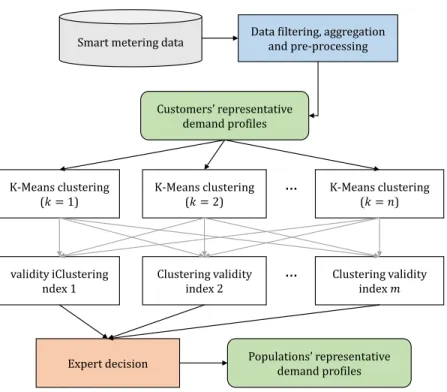
The methodology followed to find the customer groups and respective 151
representative consumption profiles is in Figure 1. The clustering process 152
is similar to the one proposed in [29]. Firstly, smart metering data is pro-153
cessed in order to obtain the customers’ representative consumption profiles, 154
secondly, various clustering configurations are tested. Configurations are 155
evaluated using multiple clustering validity indexes (CVI) which are used, 156
together with careful visual evaluation, to chose the final configuration and 157
obtain the customer groups and profiles. 158
3.1. Customers’ normalized representative consumption profiles 159
Smart metering consumption data is composed of a large set of times-160
tamped intervals with consumption values. In order to obtain consumption 161
profiles which can be easily interpreted, visualized and manipulated, the data 162
goes through a process of context filtering, aggregation and pre-processing. 163
The process of context filtering consists on selecting data which represents 164
a specific context, defined, for example, by a temporal window (e.g. Winter, 165
Summer), type of day (e.g. working day) and location. 166
Let xi be the feature vector (list of variables) associated to customer i. 167
xi = (xmi , xsi) where xmi has dimension r equal to the number of variables 168
which characterize a customers representative load profile (LP) or derived 169
load indices (LI) and xsi has dimension t equal to the number of survey vari-170
ables used. The dimension of a customers feature vector xiis p = r+t. The LI 171
and survey variables are presented in 5.1 and 5.3. X = {x1, x2, ..., xN} ⊆ <p 172
is the feature dataset of N customers. 173
After filtering, the consumption data is aggregated in order to reduce the 174
dimension and obtain a curve representative of the whole temporal window. 175
The aggregation is characterized by the period used, e.g., hourly, daily and 176
operator, e.g., mean, median. For example, doing an hourly mean aggrega-177
tion of the consumption data of customer i will generate a vector xm i ∈ <24 178
in which each element represents the mean consumption in a certain hour. 179
The final pre-processing consists on the normalization of the data for eas-180
ier clustering, modelling and representation of different information. This 181
paper focuses on the case of normalization for each customer in which each 182
representative profile is normalized with the maximum value of the profile 183
as normalization factor. The normalization is done with the intent of trans-184
lating the consumption dynamic in relation to the maximum. This is done 185
in [27–29]. The clustering of absolute representative consumption profiles 186
results, using the same kind of data, on a separation of groups by amount of 187
consumption.Without normalization the different shapes of curves are seem-188
ingly overshadowed by the mean absolute consumption while clustering [43]. 189
Figure 2 pictures an example of the clustering results, showing clusters
190
centroids for hourly aggregated absolute and normalized representative
pro-191
files. The curves behave in a similar way for different scales in absolute
pro-192
files. For normalized consumption profiles the curves are distinct in terms of
193
linearity and consumption between different times of the day.
194
3.2. K-means clustering 195
The K-means algorithm [44] is used due to its simplicity, efficiency and 196
scalability. The algorithm has been proven to be adequate for this type of 197
application in the literature [8, 15–18, 45, 46]. Let S = {S1, ..., SJ} be the 198
groups (sets) of customers clustered together, J the number of clusters and 199
de a chosen distance measure. The centroid of a cluster Skis its mean vector, 200
µk = |S1
k|
P
x∈Skx. The algorithm is an iterative refinement method which, in 201
this application, minimizes the distance between the customers’ consumption 202
profiles x and the populations µk, as given by (1). 203 arg min S J X k=1 X x∈Sk de(x, µk)2 (1)
The difficulty associated with this algorithm is the need to determine the 204
number of clusters and their initial centres. The choice of the number of 205
cluster centres is detailed in the following Section 3.3. The initial cluster 206
centres are generated randomly and the best clustering result of an high 207
number of runs is used. 208
3.3. Clustering evaluation 209
A clustering in X is a set of disjoint clusters that partition X into k 210
groups: S where ∪Sk∈SSk = X, Sk∩ Sl = ∅ ∀ k 6= l. The euclidean distance 211 is used and de(xi, xk) = q Pp j=1(xij − xkj)2. 212
As pictured in Figure 1, multiple CVI are used to evaluate a number 213
of different clustering configurations. If there is no consensus between the 214
different CVI the expert chooses the best configuration based on the analysis 215
of the CVI and visualization of the clustering results. 216
Three different CVI are used in this work, they evaluate the goodness 217
of the clustering in terms of maximization of inter cluster distances and 218
minimization of intra cluster distances [47]. 219
The Dunn index (D) [48] is a ratio-type index where the cohesion is esti-220
mated by the nearest neighbour distance and the separation by the maximum 221
cluster diameter. The original index is defined as, 222 D(S) = minSk∈S{minSl∈S\Sk{δ(Sk, Sl)}} maxSk∈S{∆(Sk)} (2) where, 223 δ(Sk, Sl) = min xi∈Sk min xj∈Sl {de(xi, xj)} (3) ∆(Sk) = max xi,xj∈Sk {de(xi, xj)}. (4)
The Davis-Bouldin index (DB) [49] estimates the cohesion based on the 224
distance from the points in a cluster to the centroid and the separation based 225
on the distance between centroids. The DB index is defined as: 226 DB(S) = 1 J X Sk∈S max Sl∈S\Sk nF (Sk) + F (Sl) de(µk, µl) o (5) where, 227 F (Sk) = 1 |Sk| X xi∈Sk de(xi, µk). (6)
The silhouette index (Sil) [50] is a normalized summation-type index. 228
The cohesion is measured based on the distance between all the points in the 229
same cluster and the separation is based on the nearest neighbor distance. 230
The silhouette index is defined as: 231 Sil(S) = 1 N X Sk∈S X xi∈Sk b(xi, Sk) − a(xi, Sk) max{a(xi, Sk), b(xi, Sk)} (7)
where, 232 a(xi, Sk) = 1 |Sk| X xj∈Sk de(xi, xj) (8) b(xi, Sk) = min Sl∈S\Sk n 1 |Sl| X xj∈Sl de(xi, xj) o . (9) 4. Modelling 233 4.1. Classification 234
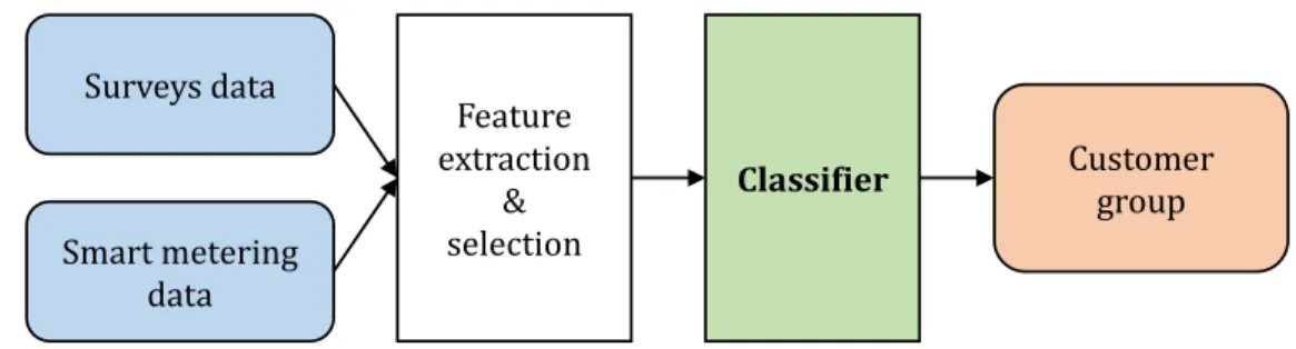
This work intends to train models to predict the group of a new customer, 235
characterized by a representative consumption profile. Figure 3 pictures the 236
electricity customer classifier. 237
Features are extracted from the survey responses and smart metering data 238
of the customer. Based on the features the classifier returns a categorical 239
variable y indicative of the customer group in which the customer best fits. 240
The classifier is a function ϕ which maps the features of a customer to 241
a categorical variable y, representing one of the J customer groups. It is 242
defined as: 243
ϕ : <p 7→ y (10)
y ∈ {c1, c2, ..., cJ} (11)
Classifiers are trained using the group labels extracted through the clus-244
tering of a full year of smart metering data, considered as the ground truth to 245
be inferred from features extracted from a limited amount of smart metering 246
data and survey data. 247
The two following sections present the modelling approaches used in this 248
methodology. 249
4.1.1. Logistic regression 250
The logistic regression (LR) models the posterior probabilities of the 251
J classes via linear function in x while ensuring the sum to one and re-252
maining in [0, 1]. The LR model has the form presented in (12), where 253
D represents the input vector [51, 52]. The parameter set of the model is 254
θ = {β10, β1T, ..., β(J −1)0, β(J −1)T }. 255
log Pr(y = 1|D = x) Pr(y = J |D = x) = β10+ β T 1x log Pr(y = 2|D = x) Pr(y = J |D = x) = β20+ β T 2x (12) .. . log Pr(y = J − 1|D = x) Pr(y = J |D = x) = β(J −1)0+ β T (J −1)x
Using the LR model, if the clustering analysis results in J customer 256
groups, the classifier linearly separates each one of J − 1 customer groups to 257
the J customer group. 258
LR is usually fit by maximum likelihood, in the case of the results pre-259
sented in this paper the Newton-Raphson optimization method is used. For 260
the case of two classes the parameters of the model can be easily interpreted 261
through the significance and sign. In the case of multiple classes the inter-262
pretation of the model parameters is more complex due to a total set of J − 1 263
parameters for each variable. 264
The LR model is chosen due to the simplicity (explained by linear func-265
tions) and interpretability, enabling the understanding of the role of the dif-266
ferent input variables in explaining the outcome [51]. Models with increased 267
complexity, such as artificial neural networks or support vector machines, 268
may provide higher accuracy but lack the transparency of the LR model 269
[53]. 270
4.1.2. Decision trees 271
Binary decision tree (DT) learning consists on fitting data to a tree-like 272
structure. This type of method partitions the feature space into a set of 273
rectangles and usually fits a constant in each one. This paper makes use 274
of the popular tree-based regression and classification method called CART 275
(Classification And Regression Tree) [51]. Tree-based methods have the ad-276
vantage of an easy interpretation and can be transformed into a simple set 277
of rules if the number of branches is low. 278
In order to grow a classification DT the learning algorithm automatically 279
splits the data into two sets at each level, optimizing some criterion which 280
translates the model accuracy. In this paper the Gini index is used, which is 281
a measure of how often a randomly chosen element from the set is incorrectly 282
labelled if it is randomly labelled according to the distribution of labels in 283
the subset. The learning algorithm minimizes the difference of this measure 284
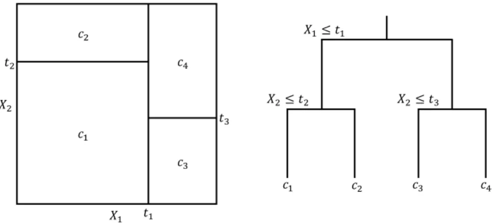
between tree levels through the growth of the DT. Using DT in the multiple 285
class case is straightforward and each end node of the tree will give a proba-286
bility for the J labels. Figure 4 pictures an example of a partition obtained 287
by binary splitting and corresponding DT. 288
A classification DT model is chosen, similarly to the LR model, due to 289
its interpretability, providing a popular binary tree representation [51]. 290
4.2. Feature selection 291
The objective of feature selection (FS) is to choose a subset of the avail-292
able features by eliminating features with little or no predictive information 293
and also redundant features that are strongly correlated [54]. FS techniques 294
are usually divided into filter, wrapper and embedded methods. Wrapper 295
and embedded are usually referred to as model-based methods and filter 296
techniques as model-free methods. 297
Filter techniques assess the relevance of features by looking only at the 298
intrinsic properties of the data. Filter techniques are normally easily scalable
299
to very high-dimension datasets and computationally simple, having the
dis-300
advantage of not taking into account the interaction with the classifier [55].
301
Wrapper methods embed the classification model within the feature sub-302
set search. The selected set of features is obtained by training and testing 303
a specific classification model, rendering this approach tailored to a specific 304
classification algorithm [55]. 305
4.2.1. Regression based filter feature selection 306
In regression analysis parameters are determined indicating the relation-307
ship between the features and the model output. The p-values of the hy-308
pothesis tests based on the parameters’ standard errors indicate if the corre-309
sponding variables are believed to be significantly different from 0 (rejected 310
null hypothesis), thus indicators of the output variable. The regression fea-311
ture selection method used removes the variables for which the corresponding 312
parameters result in a p-value higher than a certain significance level (5%). 313
This parametric filter FS technique has been used in multiple studies, 314
together with LR or probit regression, in order to find which are the fea-315
tures which are indicative of a specific electricity consumption profile and 316
are determinants of electricity consumption [22, 23, 28]. 317
4.2.2. Wrapper feature selection 318
This paper proposes the use of greedy wrapper FS methods to find rela-319
tions between the characteristics of customers and the typical consumption 320
profile. FS is also done in order to generate interpretable models by signifi-321
cantly reducing the number of features used to classify new customers. 322
Sequential forward selection and sequential backward elimination [56] are 323
the FS methods used. The forward FS algorithm sequentially selects features, 324
starting with a empty set, choosing the features that improve the most the 325
prediction accuracy. This is done until there is no more improvement in 326
prediction. The backward FS algorithm starts with the full set of features and 327
sequentially removes the ones which result in an improvement in prediction 328
accuracy. 329
4.3. Model evaluation 330
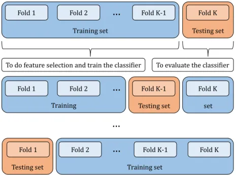
In order to maximize the significance of the performance results of the 331
trained classifiers k-fold cross-validation is used [51, 53]. This model vali-332
dation technique randomly divides the dataset into k folds. The classifier 333
is then trained (using k − 1 folds) and evaluated (using 1 fold) k times, as 334
pictured in Figure 5. The modelling approach is then evaluated through the 335
mean and standard deviation of the accuracy. 336
In order to do an unbiased FS the methods presented in Section 4.2 337
are used only based on the training sets so that the process is totally in-338
dependent from the test data. The wrapper FS methods also make use of 339
cross-validation to evaluate the feature subsets. 340
5. Results and discussion 341
5.1. Dataset 342
The proposed methodology is applied to data from 4232 Irish households 343
monitored for one and a half year. The dataset consists of electricity con-344
sumption data logged at 30 minute intervals and surveys responded before 345
the start of the trial. This dataset resulted from an electricity customer be-346
haviour trial by the Irish Commission for Energy Regulation (CER). The data 347
is stored and maintained by the Irish Social Science Data Archive (ISSDA) 348
[32]. 349
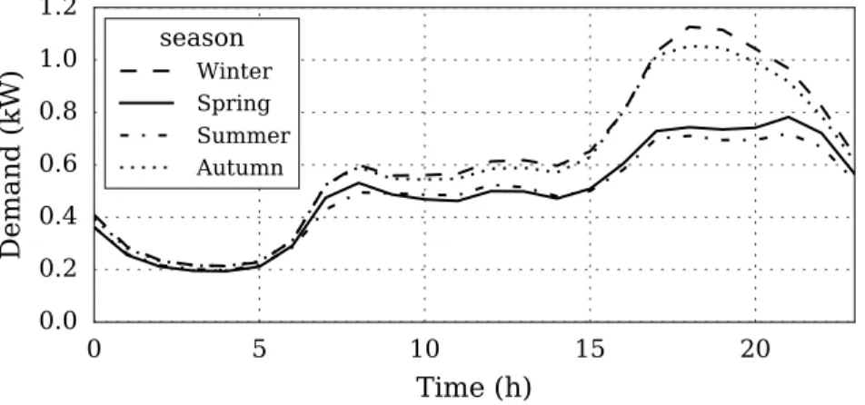
The mean hourly consumption for the four seasons is pictured in Figure 350
6. Consumption follows the typical residential dynamic with a small peak in 351
the morning and lunch time, a larger one at the end of the afternoon and 352
low consumption during the night. As expected, the mean consumption in 353
winter presents the highest values due to the heating needs. 354
The distribution of the survey responses on social class and number of 355
children per household is pictured in Figure 7. AB is upper middle class 356
and middle class, C1 is lower middle class, C2 is skilled working class, DE 357
is working and non-working classes and F represents farmers. The distribu-358
tions show that the used data encompasses different demographic groups and 359
household types. 360
The survey questions used as features are presented in Table 1 to Table 4, 361
along with a description and possible responses. Table 1 presents the features 362
with information on the respondent, Table 2 is related to the habitation 363
characteristics, Table 3 to the heating systems and Table 4 to the appliances. 364
Survey variables with no response are considered as ’refused’. The cus-365
tomers not considered in the study are the ones who did not respond to the 366
question indicating the number of adults in the household. The final dataset 367
used contains 3440 electricity customers. 368
5.2. Clustering 369
This section presents the results from the extraction of features from the 370
customers smart metering data, transformation in representative profiles and 371
clustering in order to obtain the final populations representative consumption 372
profiles. 373
5.2.1. Customers’ representative consumption profiles 374
In order to obtain the customers’ consumption profiles the parameters 375
used to extract the representative features are: 376
• Context: Only the smart metering data from working days is used and 377
profiles are extracted seasonally; 378
• Aggregation: The data is aggregated hourly resulting in twenty-four 379
features (r = 24); 380
• Operator: The operator used is the mean. 381
• Normalization: The profiles are normalized with regards to each cus-382
tomers maximum hourly consumption. 383
The final customers’ representative consumption profiles are equal to the 384
customer normalized mean hourly consumption in working days. The profiles 385
are obtained for each one of the four seasons. 386
5.2.2. Populations representative consumption profiles 387
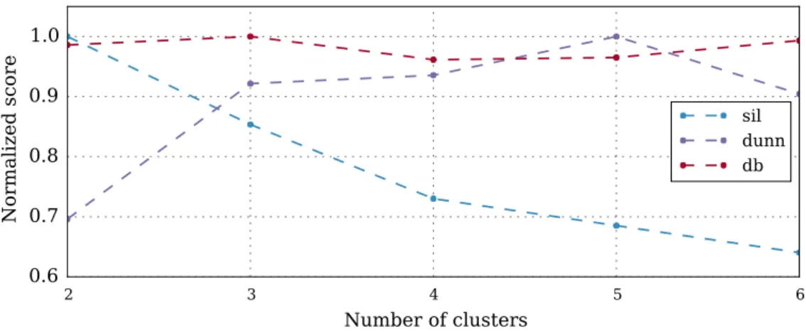
Following the proposed methodology, the best number of clusters is found 388
to be equal to four for the four seasons. Figure 8 pictures the evolution of 389
the three CVI used when generating between two and six clusters for the 390
Winter season. The Silhouette, Dunn and Davis-Bouldin indexes indicate, 391
respectively, that the best number of cluster is two, four and five. In order to 392
choose a number of clusters the partitions are visually analysed as pictured 393
in Figure 9, Figure 10 and Figure 11. The figures present the populations 394
representative consumption profiles (cluster centres) and the customers’ rep-395
resentative consumption profiles pertaining to the cluster. 396
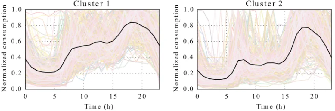
With two clusters, as pictured in Figure 9, many customers have a con-397
sumption profile different from the centre, indicating the need for an higher 398
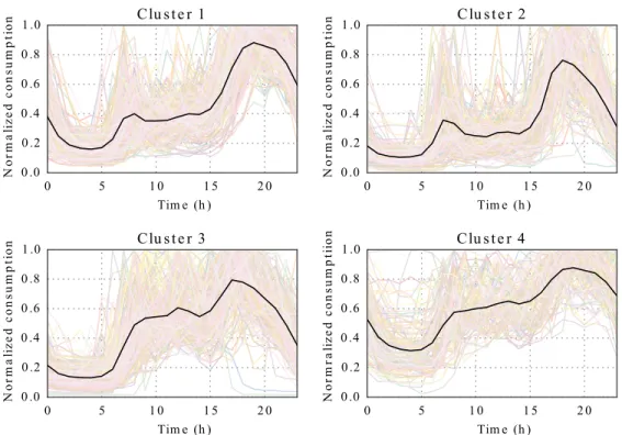
number of clusters. With four clusters, as pictured in Figure 10, the clusters 399
are sufficiently compact having a significant number of customers in each 400
group. With five clusters, as pictured in Figure 11, Cluster 2 has a low num-401
ber of customers with profiles showing a low similarity. Based on the visual 402
analysis the number of chosen clusters is equal to four. The same process is 403
used for the other seasons. 404
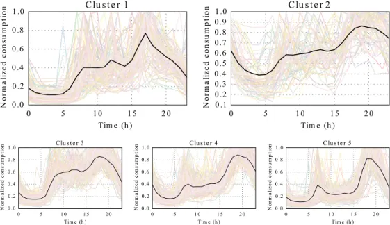
The final populations representative consumption profiles are pictured in 405
Figure 12. The population is divided mainly due to the following consump-406
tion profile characteristics: 407
• Peakiness: Relation between peak evening consumption and the con-408
sumption throughout the rest of the day. For example: in Winter, 409
clusters 1 and 2 have a much higher difference between peak evening 410
and the rest of the days consumption (high peakiness), in comparison 411
to clusters 3 and 4 (low peakiness). 412
• Decline time: Time at which the consumption starts to rapidly de-413
cline after peak evening consumption. For example: in Spring, clusters 414
2 and 4 have a late declining consumption (late decline) in comparison 415
to clusters 1 and 3 (early decline), specially cluster 3 that has a very 416
early decline in consumption. 417
• Off-peak consumption: Presence of significant consumption during 418
the off-peak hours (night and early morning) in comparison to the rest 419
of the day. For example: in Autumn, cluster 4 presents a significant 420
consumption during the night hours (high off-peak consumption) in 421
comparison to the clusters 1, 2 and 3 (low off-peak consumption). 422
Summer presents the most different populations consumption profiles in
423
comparison to the other seasons, as pictured by the the consumption profile
424
of Cluster 2. This cluster presents a high amount of variability between
425
customers results in a low mean normalized consumption throughout the
426
day.
427
Table 5 presents the distribution of customers between the different clus-428
ters for each one of the seasons. Asides from the Winter clustering, the 429
customers are approximately uniformly distributed between the four groups. 430
5.3. Classification of new customers and feature selection 431
Features extracted from metering data and from conducted surveys are 432
used for the classification of new customers. In order to evaluate the process 433
for the classification of new customers, the metering data is limited to an 434
amount starting from no data to ten weeks of data. Due to the high amount 435
of metering data and desire for interpretable models two types of features 436
extracted from the smart metering data are tested: load profile (LP) and 437
load indices (LI). 438
The LP features are the ones used in the clustering: in this paper they are 439
the hourly aggregated mean consumption normalized on an individual basis. 440
The features differ from the ones used for clustering due to being derived 441
from a limited amount of smart metering data. 442
The LI are shape indices derived from the LP, these are proposed in [57] 443
and used for the characterization of medium-voltage customers in [29]. LI
444
are used in this paper with the intention of obtaining models of easier
inter-445
pretation, explaining what consumption characteristics are the most relevant
446
when comparing customers. The indices are presented in Table 6. i1 is the 447
load factor, i2 is the off-peak factor, i3 is the night impact coefficient, i4 is 448
the lunch impact coefficient and i5 is the modulation coefficient at off-peak 449
hours. Pmax, Pmin, Pavare, respectively, the maximum, minimum and average 450
consumption of the corresponding periods. 451
Table 7 summarizes the smart metering features used in classification. In 452
the case at least one day of metering data is available, a total of p = r + t = 453
24 + 47 = 71 features are available using the LP as the smart metering 454
features and p = 5 + 47 = 52 features are available using the LI. 455
Table 8 and Table 9 present the mean and standard deviation of the 456
accuracy of the trained classifiers, through 5-fold cross-validation, in the 457
cases of no smart metering data, 1, 4, 8 and 10 weeks of available smart 458
metering data (W). In parentheses the mean number of features selected is 459
presented. The results are presented for the LR and DT models, for each 460
season, and further divided by the use of no FS, the filter FS algorithm and 461
forward FS. Backward FS results in a performance closely similar to the use 462
of no FS. Accuracy was used, instead of measures that can correctly deal 463
with class imbalances, such as the Area Under the ROC Curve (AUC) [58], 464
precision/recall and MCC, due to the multiclass nature of the classification 465
problem and the approximately balanced nature of the classes, inferred from 466
Table 5. 467
The evolution of the LR classifier performance with a growing number of 468
weeks of metering data for the Winter season is pictured in Figure 13. The
469
figure shows that, when using LP, the classification accuracy always benefits
470
from the use of survey features. The difference between the performance
471
of the classifier with and without survey features grows with the number
472
of available weeks of smart metering data. When using LI the difference is 473
only significant for the case when there is not metering data for which the 474
classification is random because no features are available. 475
Based on the analysis of the results of Table 8 and Table 9, the use 476
of LP results in an better classification performance, proving that the LI 477
are not able to correctly translate all the information needed to classify the 478
customers. 479
In general, filter FS results in the best accuracy, reducing significantly 480
the number of features in comparison with not using any FS. Using forward 481
FS resulted in an even greater reduction of the number of features at the cost 482
of a reduction of accuracy. 483
The following paragraphs present a detailed analysis of the classification 484
and feature selection results for: 485
1. Winter with no metering data; 486
2. Spring with one week of metering data transformed in LI; 487
3. Summer with four weeks of metering data transformed in LP; 488
4. Autumn with eight weeks of metering data transformed in LP. 489
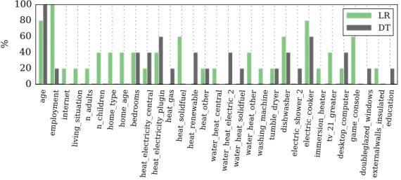
For the classification of the Winter profiles without any smart meter-490
ing data Table 10 presents the variables selected by the filter FS algorithm 491
(regression analysis) and Figure 14 pictures the rate of selection of the vari-492
ables selected by the forward FS throughout the cross-validation process. 493
A maximum mean accuracy of 39% is achieved with the features selected 494
by filter FS. With the forward FS the number of features is reduced from 495
16 to 9 and 4, respectively for LR and DT, achieving a better accuracy 496
for DT (37.4% with forward and 36.3% with filter FS) and slightly worst 497
with LR (37.3%). The variables selected by forward FS with LR modelling 498
are mainly age and employment. heat solidfuel, tumble dryer 499
and electric cooker are also selected in more than half of the cross-500
validation folds. The variable selected by forward FS with DT modelling 501
is mainly age. heat electricity plugin and electric cooker are 502
also selected in the more than half of the cross-validation folds. The age, em-503
ployment, type of heating and the use of electric cooking appliances are the 504
features which can be used as indicators to separate customers with different 505
consumption profiles. 506
For the classification of the Spring profiles with one week of smart me-507
tering data, translated by LI, Table 11 presents the variables selected by the 508
filter FS algorithm and Figure 17 pictures the rate of selection of the vari-509
ables selected by the forward FS throughout the cross-validation process. A 510
maximum mean accuracy of 56.5% is achieved with the features selected by 511
filter FS. With the forward FS the number of features is reduced from 20 to 9 512
and 5, respectively for LR and DT, achieving slightly worst accuracies. The 513
variables selected by forward FS with LR modelling are mainly the five LI 514
(i1, ..., i5) and washing machine. The variables selected by forward FS 515
with DT modelling are mainly three LI (i1, i3, i4), indicating that the load 516
factor, night impact and lunch impact are the LI features which can be used 517
as indicators to separate customers with different consumption profiles. 518
For the classification of the Summer profiles with four weeks of smart 519
metering data, translated by LP, Table 12 presents the variables selected by 520
the filter FS algorithm and Figure 15 pictures the rate of selection of the 521
variables selected by the forward FS throughout the cross-validation process. 522
A maximum mean accuracy of 73.3% is achieved with the features selected 523
by filter FS. With the forward FS the number of features is reduced from 524
30 to 16 and 5, respectively for LR and DT, achieving slightly worst ac-525
curacies (71.7% and 64.9%). The variables selected by forward FS with LR 526
modelling are mainly multiple LP features (l1, l2, l7, l11, l16, l18, l22, l23, l24) and 527
washing machine. The variables selected by forward FS with DT mod-528
elling are mainly LP features (l2, l12, l15, l23). The consumption behaviour 529
translated by LP features distributed throughout the day in combination 530
with the number of washing machines in the customers household can be 531
used as indicators to separate customers with different consumption profile. 532
For the classification of the Autumn profiles with eight weeks of smart 533
metering data, translated by LP, Table 13 presents the variables selected by 534
the filter FS algorithm and Figure 16 pictures the rate of selection of the 535
variables selected by the forward FS throughout the cross-validation pro-536
cess. A maximum mean accuracy of 81.6% is achieved with the features 537
selected by filter FS. With the forward FS the number of features is reduced 538
from 32 to 16 and 8, respectively for LR and DT, achieving worst accuracies 539
(77.9% and 70.4%). The variables selected by forward FS with LR modelling 540
are mainly multiple LP features (l8, l10, l12, l13, l14, l15, l17, l20, l22, l23, l24) and 541
washing machine. The variables selected by forward FS with DT mod-542
elling are mainly LP features (l2, l3, l5, l21, l23). The consumption behaviour 543
translated by LP features distributed throughout the day in combination 544
with the number of washing machines in the customers household can be 545
used as indicators to separate customers with different consumption profile. 546
Notice the LR results having a high standard deviation of the accuracy, 547
such as the results for ten weeks of metering data for Winter and Spring 548
with no FS, using LP metering features. These result due the inappropriate 549
convergence of the optimization method for LR training. Using forward FS 550
this problem is avoided. 551
Based on the results, the five most important variables or questions an 552
utility should ask customers on sign-up are: 553
1. What is the customer employment status; 554
2. How old the customer is; 555
3. How many dishwashers are used in the clients household; 556
4. How many electric cookers are used in the clients household; 557
5. How many washing machines are used in the clients household. 558
6. Conclusions 559
The integration of smart metering in the power grid enables a detailed 560
analysis of the consumption behaviour of electricity customers. Knowledge 561
on the typical consumption profiles of customers and the main drivers of con-562
sumption are extremely valuable for decision makers in the utility industry 563
and policy. The engagement and education of consumers is seen as a key 564
task in order to successfully reap the potential benefits of the smart grid 565
[41]. The daily routines and the social context of consumers needs to be 566
correctly taken into account to efficiently plan and target the correct groups 567
for potential DSM programs and create incentives for consumers to act with 568
regard towards sustainability. 569
The proposed process is a contribution for enabling the modelling of inter-570
pretable classifiers to predict the consumption profile group of new customers 571
using smart metering data and survey responses. It enables the discovery of 572
the drivers of consumption profiles, e.g., which characteristics of customers 573
are able to translate consumption behaviour differences. This can contribute 574
to the better engagement of consumers and development of measures to in-575
crease efficiency in the power grid. 576
An application, based on the data from more than three thousand resi-577
dential electricity customers from Ireland, shows the viability of the proposed 578
methods. Without any metering data the LR is able to correctly classify up 579
to 39% of the customers which is significantly better than randomly insert-580
ing the customer in one of the four customer groups (with four customer 581
groups). With the growth of available smart metering data the simulations 582
show an increase in accuracy achieving up to 60%, 70% and 80% accuracy, 583
respectively, with 1, 4 and 8 weeks of data. 584
The forward FS results pictured are easily interpreted and resulted in 585
the discovery of the most important features when grouping electricity cus-586
tomers by their representative consumption profile. For the Irish population
587
studied in the paper, information on the representative consumption profile
588
throughout all the day results in the highest classification accuracy. A low
589
number of shape indices is not suitable to accurately classify new electricity
590
customers. The number of washing machines in the customers households is 591
revealed to be a very important feature in the classification task, seemingly 592
being the most influencing feature to the considerable increase of accuracy 593
from the use of survey features added to the smart metering features. 594
Acknowledgements 595
This work was supported by FCT, through IDMEC, under LAETA, 596
project UID/EMS/50022/2013 and SusCity (MITP-TB/CS/0026/2013). The 597
work of J. L. Viegas was supported by the PhD in Industry Scholarship 598
SFRH/BDE/95414/2013 from FCT and Novabase. S. M. Vieira acknowl-599
edges support by Program Investigador FCT (IF/00833/2014) from FCT, 600
co-funded by the European Social Fund (ESF) through the Operational Pro-601
gram Human Potential (POPH). 602
References 603
[1] Exxon Mobil Corporation, The outlook for energy: a view to 2040. 604
[2] OECD, ICT applications for the smart grid: opportunities and policy 605
implications, OECD Digital Economy Papers (190). 606
[3] D. S. Markovic, D. Zivkovic, I. Branovic, R. Popovic, D. Cvetkovic, 607
Smart power grid and cloud computing, Renewable and Sustainable En-608
ergy Reviews 24 (2013) 566–577. 609
[4] U.S. Energy Information Administration, Annual electric power industry 610
report, Tech. rep. (2013). 611
URL http://www.eia.gov/electricity/data/eia861/ 612
[5] Commission Europ´eenne, Benchmarking smart metering deployment in 613
the EU-27 with a focus on electricity (2014). 614
[6] R. Granell, C. J. Axon, D. C. Wallom, Clustering disaggregated load 615
profiles using a Dirichlet process mixture model, Energy Conversion and 616
Management 92 (2015) 507–516. 617
[7] P. R. Jota, V. R. Silva, F. G. Jota, Building load management using 618
cluster and statistical analyses, International Journal of Electrical Power 619
& Energy Systems 33 (8) (2011) 1498–1505. 620
[8] I. Ben´ıtez, A. Quijano, J.-L. D´ıez, I. Delgado, Dynamic clustering seg-621
mentation applied to load profiles of energy consumption from Spanish 622
customers, International Journal of Electrical Power & Energy Systems 623
55 (2014) 437–448. 624
[9] M. Misiti, Y. Misiti, G. Oppenheim, Optimized clusters for disaggre-625
gated electricity load forecasting, REVSTAT - Statistical Journal 8 (2) 626
(2010) 105–124. 627
[10] F. Andersen, H. Larsen, T. Boomsma, Long-term forecasting of hourly 628
electricity load: Identification of consumption profiles and segmentation 629
of customers, Energy Conversion and Management 68 (2013) 244–252. 630
[11] H. R. Sadeghi Keyno, F. Ghaderi, a. Azade, J. Razmi, Forecasting elec-631
tricity consumption by clustering data in order to decline the periodic 632
variable’s affects and simplification the pattern, Energy Conversion and 633
Management 50 (3) (2009) 829–836. 634
[12] G. Chicco, I. S. Ilie, Support vector clustering of electrical load pattern 635
data, IEEE Transactions on Power Systems 24 (3) (2009) 1619–1628. 636
[13] N. Mahmoudi-Kohan, M. P. Moghaddam, M. Sheikh-El-Eslami, An an-637
nual framework for clustering-based pricing for an electricity retailer, 638
Electric Power Systems Research 80 (9) (2010) 1042–1048. 639
[14] J. J. L´opez, J. a. Aguado, F. Mart´ın, F. Mu˜noz, a. Rodr´ıguez, J. E. Ruiz, 640
Hopfield-K-Means clustering algorithm: a proposal for the segmentation 641
of electricity customers, Electric Power Systems Research 81 (2) (2011) 642
716–724. 643
[15] V. Figueiredo, F. Rodrigues, Z. Vale, J. Gouveia, An electric energy 644
consumer characterization framework based on data mining techniques, 645
IEEE Transactions on Power Systems 20 (2) (2005) 596–602. 646
[16] T. R¨as¨anen, D. Voukantsis, H. Niska, K. Karatzas, M. Kolehmainen, 647
Data-based method for creating electricity use load profiles using large 648
amount of customer-specific hourly measured electricity use data, Ap-649
plied Energy 87 (11) (2010) 3538–3545. 650
[17] L. Hern´andez, C. Baladr´on, J. Aguiar, B. Carro, A. S´anchez-Esguevillas, 651
Classification and clustering of electricity demand patterns in industrial 652
parks, Energies 5 (12) (2012) 5215–5228. 653
[18] F. Rodrigues, J. Duarte, V. Figueiredo, Z. Vale, M. Cordeiro, A com-654
parative analysis of clustering algorithms applied to load profiling, in: 655
Machine Learning and Data Mining in Pattern Recognition, Springer, 656
2003, pp. 73–85. 657
[19] X. Zhang, C. Sun, Dynamic intelligent cleaning model of dirty electric 658
load data, Energy Conversion and Management 49 (4) (2008) 564–569. 659
doi:10.1016/j.enconman.2007.08.007. 660
[20] A. Mutanen, M. Ruska, Customer classification and load profiling 661
method for distribution systems, IEEE Transactions on Power Deliv-662
ery 26 (3) (2011) 1755–1763. 663
[21] T. F. Sanquist, H. Orr, B. Shui, A. C. Bittner, Lifestyle factors in U.S. 664
residential electricity consumption, Energy Policy 42 (2012) 354–364. 665
[22] A. Kavousian, R. Rajagopal, M. Fischer, Determinants of residential 666
electricity consumption: using smart meter data to examine the effect 667
of climate, building characteristics, appliance stock, and occupants’ be-668
havior, Energy 55 (2013) 184–194. 669
[23] M. Bedir, E. Hasselaar, L. Itard, Determinants of electricity consump-670
tion in Dutch dwellings, Energy and Buildings 58 (2013) 194–207. 671
[24] B. S¨utterlin, T. a. Brunner, M. Siegrist, Who puts the most energy into 672
energy conservation? A segmentation of energy consumers based on 673
energy-related behavioral characteristics, Energy Policy 39 (12) (2011) 674
8137–8152. 675
[25] F. Fusco, M. Wurst, J. W. Yoon, Mining residential household informa-676
tion from low-resolution smart meter data, in: 21st International Con-677
ference on Pattern Recognition (ICPR), IEEE, 2012, pp. 3545–3548. 678
[26] C. Beckel, L. Sadamori, T. Staake, S. Santini, Revealing household char-679
acteristics from smart meter data, Energy 78 (2014) 397–410. 680
[27] T. K. Wijaya, T. Ganu, D. Chakraborty, K. Aberer, D. P. Seetharam, 681
Consumer segmentation and knowledge extraction from smart meter 682
and survey data, in: SIAM International Conference on Data Mining 683
(SDM14), 2014. 684
[28] J. D. Rhodes, W. J. Cole, C. R. Upshaw, T. F. Edgar, M. E. Webber, 685
Clustering analysis of residential electricity demand profiles, Applied 686
Energy 135 (2014) 461–471. doi:10.1016/j.apenergy.2014.08.111. 687
[29] S. Ramos, J. M. Duarte, F. J. Duarte, Z. Vale, A data-mining-based 688
methodology to support MV electricity customers characterization, En-689
ergy and Buildings 91 (2015) 16–25. 690
[30] R. N. Bolton, A Dynamic Model of the Duration of the Customer’s Re-691
lationship with a Continuous Service Provider: The Role of Satisfaction, 692
Marketing Science 17 (1) (1998) 45–65. doi:10.1287/mksc.17.1.45. 693
[31] P. C. Verhoef, Understanding the effect of customer relation-694
ship management efforts on customer retention and customer 695
share development, Journal of Marketing 67 (4) (2003) 30–45. 696
doi:10.1509/jmkg.67.4.30.18685. 697
[32] ISSDA, Data from the Commission for Energy Regulation -698
www.ucd.ie/issda. 699
[33] M. Welsch, M. Howells, M. Bazilian, J. DeCarolis, S. Hermann, 700
H. Rogner, Modelling elements of smart grids: enhancing the OSe-701
MOSYS (open source energy modelling system) code, Energy 46 (1) 702
(2012) 337–350. 703
[34] U.S. Department of Energy, The smart grid: an introduction, Tech. rep. 704
(2008). 705
[35] International Energy Agency, Technology roadmap: smart grids, Tech. 706
rep. (2011). 707
[36] ETP SmartGrids, European technology platform smart grids: vision 708
and strategy for Europe’s electricity networks of the future, Tech. rep. 709
(2006). 710
[37] A. Battaglini, J. Lilliestam, A. Haas, A. Patt, Development of supers-711
mart grids for a more efficient utilisation of electricity from renewable 712
sources, Journal of Cleaner Production 17 (10) (2009) 911–918. 713
[38] C. Felix, M. Ardelean, J. Vasiljevska, A. Mengolini, G. Fulli, 714
E. Amoiralis, M. S. Jim´enez, C. Filiou, Smart grid projects outlook 715
2014, European Commision, JRC Science and Policy Reports. 716
[39] A. Faruqui, D. Harris, R. Hledik, Unlocking the e 53 billion savings 717
from smart meters in the eu: How increasing the adoption of dynamic 718
tariffs could make or break the eu’s smart grid investment, Energy Policy 719
38 (10) (2010) 6222–6231. 720
[40] A. J. Conejo, J. M. Morales, L. Baringo, Real-time demand response 721
model, Smart Grid, IEEE Transactions on 1 (3) (2010) 236–242. 722
[41] V. Giordano, F. Gangale, G. Fulli, M. S´anchez, J. Dg, I. Onyeji, 723
A. Colta, I. Papaioannou, A. Mengolini, C. Alecu, T. Ojala, I. Maschio, 724
Smart grid projects in Europe : lessons learned and current develop-725
ments, European Commision: JRC Scientific and Policy Reports. 726
[42] Institute of Communication & Computer Systems of the National Tech-727
nical University of Athen ICCS-NTUA for the European Commission, 728
Study on cost benefit analysis of Smart Metering Systems in EU Member 729
States - Final Report. 730
[43] J. L. Viegas, S. M. Vieira, R. Mel´ıcio, V. M. F. Mendes, J. a. M. C. 731
Sousa, Electricity demand profile prediction based on household char-732
acteristics, in: Proceedings of the 12th International Conference on the 733
European Energy Market, 2015. 734
[44] J. MacQueen, Some methods for classification and analysis of multi-735
variate observations, in: Proceedings of the fifth Berkeley symposium 736
on mathematical statistics and probability, Vol. 1, Oakland, CA, USA., 737
1967, pp. 281–297. 738
[45] G. Chicco, Overview and performance assessment of the clustering meth-739
ods for electrical load pattern grouping, Energy 42 (1) (2012) 68–80. 740
doi:10.1016/j.energy.2011.12.031. 741
URL http://dx.doi.org/10.1016/j.energy.2011.12.031 742
[46] T. Warren Liao, Clustering of time series data - A survey, Pattern Recog-743
nition 38 (2005) 1857–1874. 744
[47] O. Arbelaitz, I. Gurrutxaga, J. Muguerza, J. M. P´erez, I. n. Perona, An 745
extensive comparative study of cluster validity indices, Pattern Recog-746
nition 46 (1) (2013) 243–256. 747
[48] C. Dunn, A fuzzy relative of the ISODATA process and its use in detect-748
ing compact well-separated clusters, Journal of Cybernetics 3 (3) (1973) 749
32–57. 750
[49] D. L. Davies, D. W. Bouldin, A cluster separation measure, IEEE Trans-751
actions on Pattern Analysis and Machine Intelligence (2) (1979) 224– 752
227. 753
[50] P. Rousseeuw, Silhouettes: A graphical aid to the interpretation and 754
validation of cluster analysis, Journal of Computational and Applied 755
Mathematics 20 (1987) 53–65. 756
[51] T. Hastie, R. Tibshirani, J. Friedman, The elements of statistical learn-757
ing: data mining, inference, and prediction, Springer.[Online book], 758
2008. 759
[52] D. C. Montgomery, E. A. Peck, G. Vining, Introduction to Linear Re-760
gression Analysis, 5th Edition, Wiley, 2012. 761
[53] M. R. Berthold, C. Borgelt, F. H¨oppner, F. Klawonn, Guide to Intel-762
ligent Data Analysis: How to Intelligently Make Sense of Real Data, 763
Springer, 2010. 764
[54] S. M. Vieira, J. a. M. Sousa, T. a. Runkler, Two cooperative ant colonies 765
for feature selection using fuzzy models, Expert Systems with Applica-766
tions 37 (4) (2010) 2714–2723. doi:10.1016/j.eswa.2009.08.026. 767
[55] Y. Saeys, I. Inza, P. Larra˜naga, A review of feature selection techniques 768
in bioinformatics, Bioinformatics 23 (19) (2007) 2507–2517. 769
[56] J. Kittler, Feature set search algorithms, Pattern recognition and signal 770
processing (1978) 41–60. 771
[57] G. Chicco, R. Napoli, P. Postolache, M. Scutariu, C. Toader, Customer 772
characterization options for improving the tariff offer, IEEE Transac-773
tions on Power Systems 18 (1) (2003) 381–387. 774
[58] J. A. Hanley, B. J. McNeil, The meaning and use of the area under a 775
receiver operating characteristic (ROC) curve., Radiology 143 (4) (1982) 776
29–36. doi:10.1148/radiology.143.1.7063747. 777
Figures 778
Smart metering data Data filtering, aggregation and pre-processing
Customers’ representative demand profiles K-Means clustering (𝑘 = 1) K-Means clustering (𝑘 = 2) … K-Means clustering (𝑘 = 𝑛) validity iClustering ndex 1 Clustering validity index 2 Clustering validity index 𝑚 …
Expert decision Populations’ representative demand profiles
0 5 10 15 20 Time (h) 0 1 2 3 4 5 6 Absolute consump tion (kWh)
(a)Absolute consumption
0 5 10 15 20 Timet(h) 0.1 0.2 0.3 0.4 0.5 0.6 0.7 0.8 0.9 Normalizedt consump tion
(b)Customer normalized consumption
Figure 2: Example of populations representative consumption profiles using absolute and customer normalized consumption (resulting cluster centroids).
Classifier Surveys data Smart metering data Feature extraction & selection Customer group
𝑐1 𝑐2 𝑐3 𝑐4 𝑋1 𝑋2 𝑡2 𝑡1 𝑡3 𝑋1≤ 𝑡1 𝑋2≤ 𝑡2 𝑋2≤ 𝑡3 𝑐1 𝑐2 𝑐3 𝑐4
Figure 4: Left: data partitioned in four categories by binary splitting. Right: CART tree corresponding to the partition.
set Testing set Training set
Fold 1 Fold 2
…
Fold K-1 Fold KTo do feature selection and train the classifier To evaluate the classifier
Testing set Training
Fold 1 Fold 2
…
Fold K-1 Fold K…
Testing set Training set
Fold 1 Fold 2
…
Fold K-1 Fold K0
5
10
15
20
Time (h)
0.0
0.2
0.4
0.6
0.8
1.0
1.2
Demand (kW)
season
Winter Spring Summer Autumn0 200 400 600 800 1000 1200 count DE C1 C2 AB F refused
(a) Social class
0 500 1000 1500 2000 2500 count none 1 2 3 4 5 6 (b) Number of children
2 3 4 5 6 Number of clusters 0.6 0.7 0.8 0.9 1.0 Normalized score sil dunn db
0 5 1 0 1 5 2 0 Tim e (h ) 0 .0 0 .2 0 .4 0 .6 0 .8 1 .0 N o rm a li ze d c o n su m p ti o n Clu s t e r 1 0 5 1 0 1 5 2 0 Tim e (h ) 0 .0 0 .2 0 .4 0 .6 0 .8 1 .0 N o rm a li ze d c o n su m p ti o n Clu s t e r 2
0 5 1 0 1 5 2 0 Tim e (h ) 0 .0 0 .2 0 .4 0 .6 0 .8 1 .0 N o rm a li ze d c o n su m p ti o n Clu s t e r 1 0 5 1 0 1 5 2 0 Tim e (h ) 0 .0 0 .2 0 .4 0 .6 0 .8 1 .0 N o rm a li ze d c o n su m p ti o n Clu s t e r 2 0 5 1 0 1 5 2 0 Tim e (h ) 0 .0 0 .2 0 .4 0 .6 0 .8 1 .0 N o rm a li ze d c o n su m p ti o n Clu s t e r 3 0 5 1 0 1 5 2 0 Tim e (h ) 0 .0 0 .2 0 .4 0 .6 0 .8 1 .0 N o rm ra li ze d c o n su m p ti io n Clu s t e r 4
0 5 1 0 1 5 2 0 Tim e (h ) 0 .0 0 .2 0 .4 0 .6 0 .8 1 .0 N o rm a li ze d c o n su m p ti o n Clu s t e r 1 0 5 1 0 1 5 2 0 Tim e (h ) 0 .1 0 .2 0 .3 0 .4 0 .5 0 .6 0 .7 0 .8 0 .9 1 .0 N o rm a li ze d c o n su m p ti o n Clu s t e r 2 0 5 1 0 1 5 2 0 Tim e (h ) 0 .0 0 .2 0 .4 0 .6 0 .8 1 .0 N o rm a li ze d c o n su m p ti o n Clu s t e r 3 0 5 1 0 1 5 2 0 Tim e (h ) 0 .0 0 .2 0 .4 0 .6 0 .8 1 .0 N o rm a li ze d c o n su m p ti o n Clu s t e r 4 0 5 1 0 1 5 2 0 Tim e (h ) 0 .0 0 .2 0 .4 0 .6 0 .8 1 .0 N o rm a li ze d c o n su m p ti o n Clu s t e r 5
0 5 1 0 1 5 2 0 Tim e (h ) 0 .1 0 .2 0 .3 0 .4 0 .5 0 .6 0 .7 0 .8 0 .9 N o rm a li ze d c o n su m p ti o n 1 2 3 4 (a) Winter 0 5 1 0 1 5 2 0 Tim e (h ) 0 .1 0 .2 0 .3 0 .4 0 .5 0 .6 0 .7 0 .8 0 .9 N o rm a li ze d c o n su m p ti o n 1 2 3 4 (b) Spring 0 5 1 0 1 5 2 0 Tim e (h ) 0 .1 0 .2 0 .3 0 .4 0 .5 0 .6 0 .7 0 .8 0 .9 N o rm a li ze d c o n su m p ti o n 1 2 3 4 (c) Summer 0 5 1 0 1 5 2 0 Tim e (h ) 0 .1 0 .2 0 .3 0 .4 0 .5 0 .6 0 .7 0 .8 0 .9 N o rm a li ze d c o n su m p ti o n 1 2 3 4 (d) Autumn
0 2 4 6 8 10 Weeks of data 20 30 40 50 60 70 80 90 Accuracy ( %)
Without survey features With survey features
(a)Metering data features: LI
0 2 4 6 8 10 Weeks of data 20 30 40 50 60 70 80 90 100 Accuracy ( %)
Without survey features With survey features
(b) Metering data features: LP Figure 13: LR classifier accuracy using filter FS with and without the survey features for Winter profiles.
age employment
internet living_situation
n_adults
n_children home_type home_age bedrooms
heat_electricity_central heat_electricity_plugin heat_gas
heat_solidfuel heat_renewable heat_other water_heat_central
water_heat_electric_2 water_heat_solidfuel water_heat_other washing_machine
tumble_dryer dishwasher electric_shower_2 electric_cooker immersion_heater
tv_21_greater desktop_computer game_console doubleglazed_windows externalwalls_insulated education
0
20
40
60
80
100
%
LR DTFigure 14: Forward FS for Winter with no metering data: rate of selection of features throughout the cross-validation process.
internet n_adults n_children bedrooms heat_electricity_plugin heat_gas heat_oil heat_renewable water_heat_centralwater_heat_gas water_heat_renewable washing_machine
tumble_dryer electric_cooker electric_heater standalone_freezer desktop_computer cfl_lightbulbs externalwalls_insulated l1 l2 l3 l5 l7 l8 l10 l11 l12 l13 l14 l15 l16 l18 l20 l21 l22 l23 l24
0
20
40
60
80
100
%
LR DTFigure 15: Forward FS for Summer with 4 weeks metering data (LP): rate of selection of features throughout the cross-validation process.
age
social_class internet heat_gas heat_oil heat_timer water_heat_electric_2 water_heat_renewable washing_machine tumble_dryer dishwasher electric_shower_2 laptop_computer doubleglazed_windows l1 l2 l3 l4 l5 l6 l7 l8 l9 l10 l11 l12 l13 l14 l15 l16 l17 l18 l20 l21 l22 l23 l24
0
20
40
60
80
100
%
LR DTFigure 16: Forward FS for Autumn with 8 weeks metering data (LP): rate of selection of features throughout the cross-validation process.
Tables 779
Nomenclature
Acronyms
AMI Advanced metering r number of smart metering
infrastructure data features
EU European Union t number of survey features
DSM Demand side management X feature dataset of all
customers
CVI Clustering validity index µi ith consumption profile of the
LP Load profile population
LI Load indexes S set of the groups of customers
FS Feature selection Si ith clustered group of
LR Logistic regression customers
DT Decision tree J number of clusters/customer
CER Commission for Energy groups
Regulation de(v1, v1) euclidean distance
ISSDA Irish Social Science D(S) Dunn index
Data Archive
DB(S) Davis Bouldin index
Symbols Sil(S) Silhouette index
xi feature vector of customer i y categorical variable
xm
i customer i smart metering representing a group
data features i1, i2, . . . , i5 load indices
xs
i customer i surveys features Pmax/min/av maximum, minimum and
N number of customers average consumption
Table 1: Survey features I: respondent
Feature Description: {responses}
sex Sex of respondent: {male, female}
age Age of respondent in years: {18-25, 26-35, 36-45, 46-55, 56-65, 65
or more, refused}
employment employment status of respondent: {Employee, self-employed,
unemployed}
social class Social class of respondent: {AB, C1, C2, DE, F, refused}
education
Education level of respondent: {none, primary, secondary to intermediate cert junior cert level, secondary to leaving cert level, third level, refused}
income Income of respondent before tax in euro: {0-15k, 15k-30k, 30k-50k,
50k-75k, 75k or more, refused}
Table 2: Survey features II: household
Feature Description: {responses}
home type Household type: {apartment, semi-detached, detached,
terraced, bungalow}
home age Household age in years: {0-4, 5-9, 10-29, 30-74, 75 or
more}
bedrooms Number of bedrooms : {1, 2, 3, 4, 5 or more, refused}
clf lighbulbs Fraction of CLF light bulbs: {none, about a quarter,
about half, about three quarters}
doublegazed windows Fraction of doubleglazed windows: {none, about a
quarter, about half, about three quarters}
attic insulated Presence and age of attic insulation: {yes (last 5 years),
yes, no, don’t know}
externalwalls insuled Presence and age of insulation of external walls: {yes, no,
don’t know}
Table 3: Survey features III: heating
Feature Description: {responses}
heat electricity central Central electric heating : {yes, no}
heat gas Gas heating : {yes, no}
heat oil Oil heating : {yes, no}
heat solidfuel Solid fuel heating : {yes, no}
heat renewable Renewable energy heating : {yes, no}
heat other Other type of heating : {yes, no}
heat timer Use of heating timer : {yes, no}
water heat central Central water heating : {yes, no}
water heat electric Electric water heating: {yes, no}
water heat gas Gas water heating: {yes, no}
water heat oil Oil water heating: {yes, no}
water heat solidfuel Solid fuel water heating: {yes, no}
water heat renewable Renewable water heating: {yes, no}
Table 4: Survey features IV: appliances
Feature Description: {responses}
washing machine Number of washing machines : {0, 1, 2, 3 or more}
tumble dryer Number of tumble dryers : {0, 1, 2, 3 or more}
dishwasher Number of dishwashers : {0, 1, 2, 3 or more}
electric shower Number of electric showers : {0, 1, 2, 3 or more}
electric cooker Number of electric cookers : {0, 1, 2, 3 or more}
electric heater Number of electric heaters : {0, 1, 2, 3 or more}
standalone freezer Number of standalone freezers : {0, 1, 2, 3 or more}
water pump Number of water pumps : {0, 1, 2, 3 or more}
immersion heater Number of immersion heaters : {0, 1, 2, 3 or more}
tv 21 less Numbers of TVs with 21 or less inches: {0, 1, 2, 3, 4 or more}
tv 21 greater Number of TVs with more than 21 inches: {0, 1, 2, 3, 4 or
more}
desktop computer Number of desktop computers: {0, 1, 2, 3, 4 or more}
laptop computer Number of laptop computers: {0, 1, 2, 3, 4 or more}
Table 5: Distribution of customers between the different clusters for the four seasons
Cluster Winter Spring Summer Autumn
1 30.93% 26.25% 26.14% 20.34%
2 25.50% 31.89% 18.83% 31.47%
3 28.17% 21.53% 27.17% 29.19%
Table 6: Normalized indices to characterize electricity customers’ behaviour
Parameter Definition Periods
Daily Pav/Pmax i1= Pav,day/Pmax,day 1 day
Daily Pmin,day/Pmax,day i2= Pmin,day/Pmax,day 1 day
Night impact i3= 1/3Pav,night/Pav,day
1 day and 8 h night (from 23h to 06h)
Lunch impact i4= 1/8Pav,lunch/Pav,day 1 day and 3 h lunch
from (12h to 15h)
Table 7: Smart metering data features used for classification
Smart metering data features
Load indices (LI) Normalized indices to characterize
electricity constumers’ behaviour. i1, i2, i3, i4, i5
Load profile (LP) Normalized mean hourly aggregated