Contribution to the study of the impact of nonlinearities on telecommunications systems

Pedro Miguel Ribeiro

Lavrador

Contribuição ao estudo do impacto das não

linearidades nos sistemas de telecomunicações

BB Signal Processing Up Conversion x(t) y(t) 010110 PA x(t) y(t)^

?

Pedro Miguel Ribeiro

Lavrador

Contribuição ao estudo do impacto das não

linearidades nos sistemas de telecomunicações

Contribution to the study of the impact of

nonlinearities on telecommunications systems

tese apresentada à Universidade de Aveiro para cumprimento dos requisitos necessários à obtenção do grau de Doutor em Engenharia Electrotécnica, realizada sob a orientação científica do Dr. José Carlos Pedro, Professor Catedrático do Departamento de Electrónica, Telecomunicações e Informática da Universidade de Aveiro e sob a co-orientação científica do Dr. Nuno Borges Carvalho Professor Associado do mesmo departamento.

Apoio financeiro da FCT e do FSE no âmbito do III Quadro Comunitário de Apoio.

o júri

presidente Doutor Jorge Ribeiro Frade

Professor Catedrático da Universidade de Aveiro (em representação da Reitora da Universidade de Aveiro)

Doutor José Carlos Esteves Duarte Pedro

Professor Catedrático da Universidade de Aveiro (orientador) Doutor João José Lopes da Costa Freire

Professor Associado com Agregação do Instituto Superior Técnico da Universidade Técnica de Lisboa.

Doutor Tomás António Mendes de Oliveira e Silva Professor Associado da Universidade de Aveiro

Doutor Nuno Miguel Gonçalves Borges de Carvalho Professor Associado da Universidade de Aveiro (co-orientador) Doutor Anding Zhu

agradecimentos Em primeiro lugar agradeço aos meus orientadores Prof. José Carlos Pedro e Prof. Nuno Borges Carvalho, por todo o apoio que me deram ao longo destes anos e sem o qual este trabalho não teria sido possível. Agradeço o bom ambiente de trabalho proporcionado e o estímulo a procurar sempre a excelência.

Agradeço à Universidade de Aveiro, em particular ao Departamento de Electrónica Telecomunicações e Informática e ao Instituto de

Telecomunicações a disponibilização dos recursos materiais necessários à execução do trabalho. Este agradecimento é extensível aos seus

colaboradores que sempre estiveram disponíveis para ajudar.

Agradeço à Fundação para a Ciência e Tecnologia o apoio financeiro durante os primeiros anos deste projecto sob a forma de Bolsa de Doutoramento. Agradeço também à Comissão Europeia, na forma da rede de excelência TARGET, o financiamento durante a parte final deste trabalho.

Agradeço à Fundação Luso Americana para o Desenvolvimento o financiamento para viagens de apresentação de artigos em conferências internacionais, apoio este que permitiu o contacto com investigadores internacionais de grande prestígio e o correspondente alargar de horizontes para o meu trabalho.

Agradeço aos colegas de trabalho e amigos, de modo especial ao Pedro Cabral e ao João Paulo Martins companheiros de percurso em grande parte deste trajecto e que tantas vezes me encorajaram a persistir na busca de novas e melhores soluções. A sua amizade e companheirismo foram

determinantes ao longo deste trabalho. Agradeço de modo especial o apoio do Pedro Cabral para a redacção desta tese.

Agradeço aos meus pais por terem ajudado a criar em mim desde pequeno o gosto pelo saber e a cultura do procurar saber mais. Agradeço-lhes os

sacrifícios que fizeram para me permitir chegar até esta etapa. Sem eles e sem o seu exemplo de esforço nada disto seria possível.

À minha namorada e esposa Raquel, quero agradecer toda a paciência que teve comigo. O suporte nos momentos mais difíceis e o alento para continuar.

palavras-chave Modelação Comportamental, Amplificadores de Potência, Série de Volterra

resumo Esta tese insere-se na área de Electrónica de Rádio Frequência e Microondas e visa o desenvolvimento de ferramentas que permitam a melhor compreensão e análise do impacto da distorção não linear produzida em amplificadores de potência no desempenho de um sistema de telecomunicações sem fios. Devido à crescente complexidade dos amplificadores a simulação baseada em representações de circuito equivalente tornou-se extremamente pesada do ponto de vista computacional. Assim têm surgido várias técnicas de simulação de sistemas baseadas em modelos comportamentais, ou seja, que tentam aproximar a resposta do sistema a um sinal de entrada, independentemente dos elementos físicos que implementam o circuito.

Neste trabalho foram estudadas as principais técnicas de modelação comportamental existentes assim como as principais características de um amplificador de potência que o modelo comportamental deve ser capaz de prever.

Uma nova formulação de um modelo comportamental baseado na série de Volterra é apresentada em conjunto com o método de extracção ortogonal dos seus coeficientes. A principal vantagem deste novo método de extracção é permitir a determinação independente de cada valor coeficiente na série, garantindo-se deste modo um modelo com uma capacidade de aproximação óptima. A determinação dos coeficientes na série de modo independente é conseguida com base na reorganização dos termos da série e na identificação ortogonal de cada componente de saída.

Adicionalmente, a identificação das componentes de saída de uma não linearidade é ainda utilizada na definição de uma métrica que permite avaliar de modo simples qual é a degradação imposta à qualidade do sinal ao ser passado num amplificador não linear. Esta métrica contabiliza

keywords Behavioural Modelling, Power Amplifiers, Volterra Series.

abstract This thesis is related to the RF and Microwave Electronics field and the main goal of this thesis is to develop tools that can contribute to understand and analyse the impact of nonlinear distortion generated by power amplifiers on wireless communication systems.

Due to the growing complexity of amplifiers, equivalent circuit based simulations become a heavy computational task due to the large number of nonlinear elements to account for. So, several system simulation techniques have been proposed based on behavioural modelling, that is, models that can approximate the system’s response to a given input signal regardless of the physical circuit implementation description.

In this thesis, the most important behavioural modelling techniques have been studied as well as the main power amplifier characteristics that the behavioural model should account for.

A new formulation of a Volterra series based behavioural model is presented as well as the corresponding coefficient orthogonal extraction procedure. The main advantage of this new extraction method is to allow the independent determination of the exact value of each coefficient, guaranteeing this way an optimum approximation condition. The exact coefficient determination is achieved by reorganizing the series terms to reach independent subsets and by identifying separately each of systems’ output components.

In addition, nonlinearity output component separation is also used to define a Figure of Merit that allows the simple evaluation of signal quality degradation when passed through a nonlinear amplifier. This Figure takes into account simultaneously the impact of noise and distortion.

Table of Contents ... i

List of Figures...iii

List of Acronyms... vi

1. Introduction ... 1

1.1 Objectives ... 6

1.2 Thesis Description and Original Contributions... 6

1.3 References ... 7

2. State of the Art Description... 11

2.1 Introduction ... 11

2.2 Behavioural Modelling Overview ... 12

2.2.1 Main Effects to be modelled by a PA behavioural model... 16

2.2.2 Different Behavioural model capabilities... 19

2.3 Volterra Series Modelling ... 25

2.4 Conclusions ... 32

2.5 References ... 33

3. The Orthogonal formulation for Volterra Series extraction ... 37

3.1 Introduction ... 37

3.2 The used model topology. ... 38

3.3 Input signal selection to build an orthogonal polynomial. ... 39

3.4 Obtaining the model orthogonality... 44

3.5 Orthogonal Model Coefficients’ extraction... 48

3.6 Passing from the orthogonal model to the Volterra Series... 51

3.7 Summary and Conclusions ... 53

3.8 References ... 53

4. Approximation results with the new model formulation in different conditions ... 55

4.1 Introduction ... 55

4.2 First Example: A memoryless amplifier... 56

4.3 Modelling a linear filter... 61

4.4 Modelling the cascade of a memoryless nonlinearity and a linear filter. ... 65

4.4.1 Wiener Configuration... 65

4.4.2 Hammerstein Configuration ... 68

4.4.3 Wiener Hammerstein Configuration ... 71

4.5 Modelling a nonlinear amplifier with memory effects caused by the bias circuitry ... 73

4.6 Modelling a real power amplifier ... 77

4.6.1 Nonlinear Memoryless Amplifier... 77

4.6.2 Nonlinear Dynamic Amplifier... 80

4.7 Conclusions ... 84

4.8 References ... 85

5. Noise and Distortion Figure: An outcome of cross-correlation identification. ... 87

5.1 Introduction ... 87

5.2 Nonlinear Noise Figure Revisited ... 90

5.5.1 NDF calculation in a memoryless situation. ... 102

5.5.2 NDF Calculation in a nonlinear system with memory... 107

5.6 Conclusions ... 112

5.7 References ... 112

6. Conclusions ... 115

6.1 Future Work ... 116

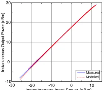
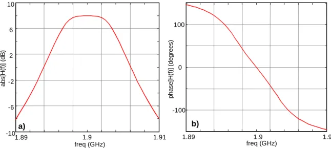
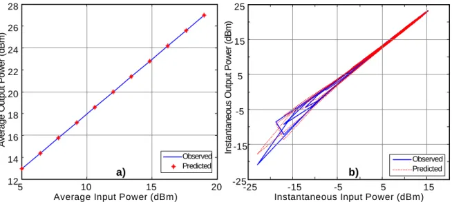
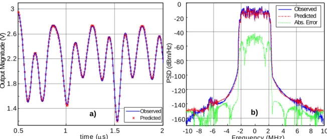
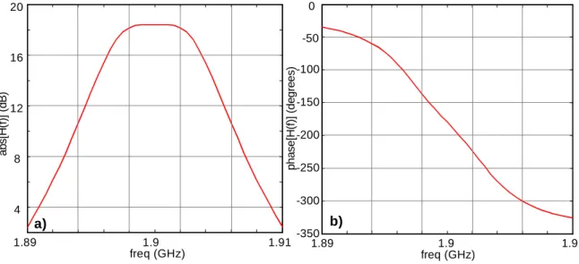
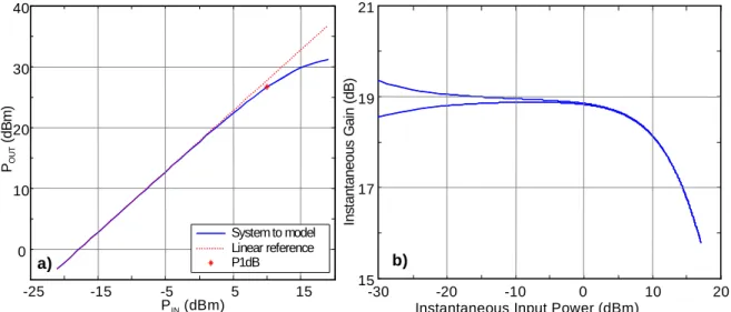
Figure 2.1 – Schematic representation of a memoryless amplifier. ... 16 Figure 2.2 – Schematic representation of nonlinear amplifier with linear memory... 17 Figure 2.3 – Schematic representation of a nonlinear amplifier with nonlinear memory proposed by Pedro et al. ... 18 Figure 2.4 – Schematic representation of a nonlinear amplifier with nonlinear memory. proposed by Vuolevi et al... 19 Figure 3.1 – Schematic representation of the dynamic polynomial model topology used.. 40 Figure 4.1 – Block diagram of the nonlinear memoryless system considered... 56 Figure 4.2 – Small signal frequency response of the memoryless amplifier. a) amplitude b) phase. ... 57 Figure 4.3 – a) One tone input/output average power. b) Dynamic gain curve of the

amplifier considered (obtained with two tones) ... 58 Figure 4.4 – Input/output average power for one tone signal: observed and modelled

results... 58 Figure 4.5 – a) Output magnitude of the complex envelope of the WCDMA sequence used to validate the model. b) – Observed and predicted power spectral density of the WCDMA signal used to validate the model... 59 Figure 4.6 – Observed and Predicted instantaneous input/output transfer characteristic for the memoryless system... 60 Figure 4.7 – a) Comparison between measured and modelled output power, IMD3 and IMD5. b) Normalized Mean Square Error variation with the input power sweep. ... 60 Figure 4.8 – Schematic representation of the linear filter used... 61 Figure 4.9 – Frequency response of the linear filter used in this situation... 61 Figure 4.10 – a) One tone input/output average power of the linear system. b) Dynamic gain curve of the linear filter. ... 62 Figure 4.11 – The magnitude plot of the linear filter impulse response... 62 Figure 4.12 – a) Input/output power comparison between observed and predicted

waveforms for an input multisine. b) Predicted and observed instantaneous input/output transfer characteristic for the linear filter. (obtained with a WCDMA signal)... 63 Figure 4.13 – a) Comparison between observed and predicted magnitude of the complex envelope of the WCDMA sequence used to validate the model. b) The predicted and observed spectra of WCDMA validation signal... 64 Figure 4.14 – a) Comparison between measured and modelled output power, IMD3 and IMD5 for the linear filter system. b) – Normalized Mean Square Error evolution with input power sweep. ... 64 Figure 4.15 – Schematic representation of the Wiener model amplifier configuration. ... 65 Figure 4.16 –Small signal gain variation with frequency of the Wiener system considered. a) amplitude; b) phase. ... 65 Figure 4.17 – a) One tone average PIN/POUT of the system of Figure 4.15. b) Instantaneous

two-tone gain curve for the Wiener configuration. ... 66 Figure 4.18 – a) Single tone input/output average power (modelled and observed). b) Comparison between modelled and measured WCDMA instantaneous output for the Wiener system. ... 66

Figure 4.20 – a) Model results on output power, IMD3 and IMD5 with input WCDMA signal power sweep. b) Normalized Mean Square Error of the model of the Wiener system.

... 67 Figure 4.21 – Schematic representation of the Hammerstein model configuration... 68 Figure 4.22 –Small signal gain variation with frequency of the Hammerstein system

considered. a) amplitude; b) phase... 68 Figure 4.23 – a) One tone average PIN/POUT of the system of Figure 4.21. b) Instantaneous

two-tone gain curve for the Hammerstein configuration. ... 69 Figure 4.24 – a) Observed and Predicted one tone input/output average power. b)

Comparison between observed and predicted WCDMA instantaneous output for the

Hammestein system... 69 Figure 4.25 – a) Time domain complex envelope magnitude comparison between

Measured and Modelled CDMA signals. b) The predicted and observed spectra of

WCDMA validation signal... 70 Figure 4.26 – a) Model results on output power, IMD3 and IMD5 with input WCDMA signal power sweep for the Hammerstein system. b) Normalized Mean Square Error of the Hammerstein system model results... 70 Figure 4.27 – Schematic representation of the Wiener-Hammerstein model configuration.

... 71 Figure 4.28 –Small signal gain variation with frequency of the Wiener-Hammerstein system considered. a) amplitude; b) phase... 71 Figure 4.29 – a) One tone average PIN/POUT of the system of Figure 4.27. b) Instantaneous

two-tone Gain curve for the Wiener-Hammerstein configuration. ... 71 Figure 4.30 – a) Observed and predicted one tone input/output average power. b)

Comparison between Modelled and Measured WCDMA instantaneous output for the Wiener-Hammerstein system. ... 72 Figure 4.31 – a) Magnitude of complex time domain envelope comparison between

Measured and Modelled CDMA signals. b) The predicted and observed spectra of CDMA validation signal. ... 72 Figure 4.32 – a) Model results on output power, IMD3 and IMD5 with input signal power sweep. b) Normalized Mean Square Error of the model for the Wiener-Hammerstein System. ... 73 Figure 4.33 – Schematic representation of the Hammerstein model configuration... 73 Figure 4.34 – Circuit diagram of the amplifier being modelled... 74 Figure 4.35 –Small signal gain variation with frequency of the simulated PA considered. 74 Figure 4.36 – a) One tone average PIN/POUT of the system of Figure 4.15. b) Instantaneous

two-tone gain curve for the simulated PA configuration. ... 75 Figure 4.37 – a) Observed and Predicted input/output one tone average power. b)

Comparison between Modelled and Measured WCDMA instantaneous output for the simulated PA. ... 75 Figure 4.38 – a) Complex envelope time domain comparison between Measured and Modelled WCDMA signals. b) The predicted and observed spectra of WCDMA validation signal. ... 76

Figure 4.40 – Schematic representation of the circuit of the memoryless amplifier... 77 Figure 4.41 –Small signal gain variation with frequency of the Wiener system considered.

... 78 Figure 4.42 – One tone average PIN/POUT of the memoryless amplifier... 78

Figure 4.43 - Time domain magnitude comparison between Measured and Modelled

multitone signals... 79 Figure 4.44 – The predicted and observed spectra of CDMA validation signal. ... 79 Figure 4.45 –WCDMA signal instantaneous input/output power curve for the memoryless amplifier – Measured and Modelled... 80 Figure 4.46 – Schematic representation of the circuit of the nonlinear dynamic amplifier.81 Figure 4.47 –Small signal gain variation with frequency of the nonlinear dynamic

amplifier. ... 81 Figure 4.48 – One tone average PIN/POUT of the dynamic amplifier. ... 82

Figure 4.49 – Time domain Magnitude comparison between Measured and Modelled CDMA signals. ... 82 Figure 4.50 – The predicted and observed spectra of CDMA validation signal. ... 83 Figure 4.51 – Instantaneous CDMA2000 input/output power curve for the nonlinear

dynamic amplifier – Measured and Modelled... 83 Figure 5.1 – The NF proposed in [5.2] variation with the input power, for a system with parameters G = 100, α = 60, as indicated in the paper. ... 90 Figure 5.2 – Geometric representation of the method used to determine the output signal component. ... 92 Figure 5.3 – Block Diagram of a general nonlinear bandpass dynamic system... 101 Figure 5.4 – Block Diagram of the simulator used to validate NDF, NLF stands for

Nonlinear Function... 103 Figure 5.5 – The input spectrum of the test signals used for the BLA extraction (simple line) and Output Spectrum (dark line). a) Signal Spectrum 1. b) Signal Spectrum 2 c) Signal Spectrum 3... 104 Figure 5.6 – In-band BLA: simulated (simple line); theoretical (dark line). a) Signal

Spectrum 1. b) Signal Spectrum 2 c) Signal Spectrum 3 ... 105 Figure 5.7 – In-band NDF: simulated (simple line), theoretical (dark line).a) Signal

Spectrum 1. b) Signal Spectrum 2 c) Signal Spectrum 3. ... 107 Figure 5.8 – Frequency response of the feedback filter F(ω) used. ... 108 Figure 5.9 – The input spectrum of the test signals used for the BLA extraction (simple line) and Output Spectrum (dotted line). a) Signal Spectrum 1. b) Signal Spectrum 2 c) Signal Spectrum 3... 109 Figure 5.10 – In-band BLA: simulated (simple line); theoretical (dotted line) a) Signal Spectrum 1. b) Signal Spectrum 2 c) Signal Spectrum 3. ... 110 Figure 5.11 – In-band NDF: simulated (simple line); theoretical (dotted line) a) Signal Spectrum 1. b) Signal Spectrum 2 c) Signal Spectrum 3 ... 111

AM-AM Amplitude Modulation to Amplitude Modulation AM-PM Amplitude Modulation to Phase Modulation

ANN Artificial Neural Network

BLA Best Linear Approximator

Bw Bandwidth

CAD Computer Aided Design

CDMA Code Division Multiple Access

CW Continuous Wave

dB Decibel dBm Decibel related to one milliwatt

DC Direct Current

FIR Finite Impulse Response

FoM Figure of Merit

fNL Nonlinear Function

GSM Global System for Mobile communications HL Best Linear Approximator function

IMD Inter-Modulation Distortion

IMD3 3rd order IMD

IMD5 5th order IMD

IIR Infinite Impulse Response

IP3 3rd Order Intercept Point

M Memory Span of the truncated Volterra series M-QAM M-ary Quadrature Amplitude Modulation N Maximum Order of the truncated Volterra series

NDF Noise and Distortion Figure

NF Noise Figure

NFIR Nonlinear Finite Impulse Response NIIR Nonlinear Infinite Impulse Response

NIM Nonlinear Integral Model

NMSE Normalized Mean Square Error

PA Power Amplifier

PAR Peak to Average Ratio

PF Polynomial Filter

PSD Power Spectral Density

RF Radio Frequency

SINAD Signal to Noise and Distortion Ratio

SNR Signal to Noise Ratio

TARGET Top Amplifier Research Groups in a European Team UMTS Universal Mobile Telecommunications System

VS Volterra Series

1. Introduction

There is some controversy about who was the inventor of wireless radio transmissions. Probably this achievement can not be attributed to a single person but is the result of several contributions. Some of the most important were: the theoretical work developed by Maxwell, the first practical controlled synthesis of radio waves by Hertz, and also, the first practical information transmission over a system by Tesla. There is a US patent of 1900 by Tesla, describing an apparatus with many “valuable uses as for instance, when it is desired to transmit intelligible messages to great distances […]”. In Europe Marconi made the first wireless transmission across the English Channel on March 1899. More consensual is that since then we have been assisting, and participating, in one rapidly increasing evolution in the wireless communications.

The development of new wireless communication technologies that occurred in the past few decades was one of the most important revolutions in the last centuries. This development changed the conventional way how people interact with each other. This on-going revolution in communications is self regenerating, as people’s eager for new services is fed by the service providers with new products and applications. Both, the number of

communication systems need to accommodate the increased information flow generated by the growing consumer’s demands.

In both wired and wireless communications the modulation schemes have changed in order to allow higher communication rates with an efficient use of the available spectra. In wired communications, the power consumption and bandwidth used are not major issues when compared to mobile communications. Due to its nature the power is available from ‘the line’ and the bandwidth is most of the times devoted to the service and not severely interfering with other systems due to its guided propagation nature. In mobile wireless communications, both these aspects might be bottlenecks. The power because the user devices are operated by batteries and the device autonomy is a key factor for its success. The bandwidth is a bottleneck, because the communication channel is shared between all the users and even between different communication systems.

In wireless communication systems the use of the frequency spectra must obey very stringent rules in order to make possible the coexistence of different services and also different service providers. Each communication standard imposes strict spectral masks created to keep the interference between different users and systems at reasonable levels and thus also to guarantee the quality of service. The recent wireless communication protocols (GSM, CDMA2000, UMTS, etc) make use of complex modulation techniques that intend to maximize the data throughput of the communication channel. To increase the debit through the channel, linear transmission should be guaranteed, so that the signal perturbations caused by distortion are avoided. This issue is even more serious when multilevel modulation techniques like M-QAM are used. As they have non-constant amplitude envelopes and the distortion impact might be different for each amplitude level.

The three restrictions referred: (i) the limited power available on the device, (ii) the efficient use of spectra and (iii) the complex modulation schemes used lead to a critical design compromise on the mobile handset power amplifier (PA). Effectively, in order to transmit the modulated signal while avoiding the transmission/generation of spectral garbage the PA should operate on its linear regime. However, to operate the PA on the linear regime an output power back off of several dBs is required, which compromises the PA efficiency and consequently reduces the battery autonomy. On the other end, to operate the PA efficiently in terms of consumed power, its signal transfer characteristic becomes strongly nonlinear. So, it is evident that a compromise between power efficiency and

linearity of the PA must be achieved. This compromise is a major concern on the design and performance of an overall communication system.

With the evolution of the computation technologies and the advent of virtual communication system simulators, the need for PA models that could mimic the PA behaviour appeared. The PA models allow the characterization of their impact on system’s performance. Two different approaches can be used to reach these models. One can start from the PA circuit design and build a virtual circuit from it through voltages or currents Kirchoff’s laws. Alternatively, one can adopt a black box methodology which, regardless of the amplifier circuit, tries to build a mathematical function that approximates the PA response to a given set of inputs. The first approach, which might be a good solution for a circuit with a small number of active elements, rapidly becomes unpractical if their amount increases, since the number of equations leads to a mathematical problem hard to solve. So, the alternative is to find a PA model that does not have the same complexity of the equivalent circuit model while still being able to approximate the PA response. This is the principle of the black box modelling or behavioural modelling approach. This modelling is distinguished from the equivalent circuit modelling because no parallelism can be made among the circuit being modelled and the model topology.

Another application of the behavioural models is its use on linearization. To alleviate the compromise between power efficiency and linearity on the PA design, some linearization techniques have been proposed throughout the last years [1.1,1.2]. One of the most discussed today is based on digital baseband predistortion. In nowadays communication systems there is a digital processor that is responsible for the baseband digital treatment of the information: coding, interleaving, spreading etc. The basic principle of digital predistortion techniques is to substitute the ideal signal to transmit by one signal somehow designed to become the ideal signal after the PA distortion effects. To be able to generate this predistorted transmission signal it is required a good inverse model of the amplifier, which is an equivalent problem of getting a good model of the amplifier.

As was stated above, the use of power amplifiers in nowadays communication systems is a key issue, since they have to be efficient, in order to extend portable devices’ battery life, and also linear to accomplish the tight spectral masks imposed by the standards to allow a practical use of the spectra. This would not be a problem if the maximum device

In order to reach a good compromise between efficiency and linearity, behavioural modelling plays a very important role either to allow the implementation of fast and accurate system level simulations or to promote the design of base-band digital pre-distorters that increase the PA efficiency.

An ideal power amplifier should work as a constant gain factor applied to the input signal

( )

t G x

( )

t

y = ⋅ (1.1a)

or also as linear gain only on the input signal bandwidth zone (an active filter):

( )

+∞

_∫

( ) (

)

∞ − − = gτ x t τ dτ t y (1.1b)

where x(t), y(t) are the input and output signals; G and g(τ) are the amplifier gain and impulse response respectively.

The power required to operate this “ideal” PA is only the power that is effectively added to the signal.

In this scenario the PA is a linear system in which the superposition principle holds. That is, if the system outputs to x1(t) and to x2(t) are known, then the systems response to

any linear combination of these two inputs is also known:

( )

( )

[

₁x₁ t ₂x₂ t

]

₁L

[

x₁

( )

t

]

₂L

[

x₂

( )

t

]

L α + α = α + α (1.2)

Linear systems have been extensively studied over the last decades, and their identification in the presence of nonlinear distortion continues to be an important investigation field [1.3-1.5]. However a simple linear based model is of no practical use when trying to estimate the distortion effect on the communication system, since a linear system does not account for distortion.

Several approaches have been used to model the nonlinear behaviour of a PA. Probably the simpler ones are the static representations in which the output signal y(t) is obtained as:

( )

t F

[

x

( )

t

]

Usual representations of the nonlinear function F are polynomial series transfer functions or functions based on hyperbolic tangent like approximations. Being very simple in their nature these methods are only capable of representing the memoryless or static part of the PA nonlinearity phenomena.

In order to account for the PA dynamic effects lots of different approaches have been proposed in the last years. They can be grouped into two main categories, the artificial neural networks (ANN) and the polynomial approximators.

With the new computational capabilities ANNs are easy tools to work with. This is one of their major advantages. However, their coefficient extraction procedure – the learning process – relies on a nonlinear optimization procedure that tries to minimize a certain error function. After the convergence of this process the ANN presents good approximation results for the input signal class used in coefficient determination, but has no guaranteed modelling accuracy for signal classes different from the one used for extraction.

On the other hand, polynomial models and, in particular, Volterra series models are linear in their parameters and so they can be extracted in a more straightforward way. Expression (1.4), represents the digital formulation of the Volterra series.

( )

( ) (

)

(

) (

) (

)

(

) (

) (

)

(

)

∑ ∑ ∑

∑ ∑

∑

= = = = = − − − − + + − − + − = M i i i i i N N N M i i i M i N N i s x i s x i s x i i i h i s x i s x i i h i s x i h s y 0 0 2 1 2 1 0 0 2 1 2 1 2 0 1 1 1 1 1 2 1 1 1 2 1 , , , , K K L L (1.4)

where, M represents the number of time samples considered and N the nonlinear order. In this expression the hx(.) parameters linearity is shown since each of them multiplies a combination of input samples.

However, due to the overlapping of a large number of different Volterra series terms, as can be seen in (1.4), it is hard to determine exactly each single coefficient. So, the coefficients are usually determined with the use of some linear estimation technique like

obtained are also optimum for a different kind of input signal. Or equivalently, the set of coefficients that model a given system might vary with different signals used for model extraction. If a method for separate identification of each coefficient is possible then the true coefficient value could be determined independently of all the others.

1.1 Objectives

The main goal of this thesis is to formulate a procedure for the orthogonal Volterra series parameter extraction. So, a rearrangement of the Volterra series that allows the separation of all its components (orthogonality) is searched. Note that this orthogonality is achieved only for a particular input signal statistics, since the input signal has impact on the output signal statistics. With this orthogonal model formulation, the coefficient determination is done in a one to one way and, finally, these orthogonal series coefficients are transformed into the conventional Volterra series parameters.

With this approach it is guaranteed that the best polynomial system approximator, up to a given order N and memory span M is obtained.

The goal of this thesis is to provide some contributions to the study of the distortion impact on a communication system.

The objectives defined for this thesis are:

• To formulate a behavioural model topology and the corresponding extraction procedure, with a well known mathematical background so that:

o The coefficient extraction is unique and straightforward o The model predictive capabilities are guaranteed.

• To propose a metric to evaluate the signal quality degradation in a nonlinear

system;

1.2 Thesis Description and Original Contributions

To reach the goals above presented this thesis is organized in the following way. Chapter 2 provides a state of the art description on power amplifier behavioural modelling. This chapter starts with a brief description of the main characteristics that must be modelled by the PA to then present a description (not exhaustive since there are a very

large number of different approaches) of the most important works on this area. The description presented on this part of the thesis follows closely a recent paper on this subject [1.6]. In the second part of this chapter some previous orthogonal approaches to Volterra series based behavioural modelling are presented.

Chapter 3, one of the most important in this thesis, presents the formal derivation of the orthogonal behavioural model proposed, the extraction procedure and correspondence between the orthogonal model’s coefficients and the corresponding time domain Volterra series. This Chapter is followed by the practical validation results shown in Chapter 4, where the modelling procedure is tested in a wide range of different situations ranging from a simulated memoryless amplifier to a real PA with memory effects. These two chapters aggregate a set of original author contributions published in several national and international conference papers [1.7-1.12].

As an application of cross-correlation identification techniques, and output signal components identification, Chapter 5 presents the author contributions to evaluate the signal quality degradation in a nonlinear system due to noise and distortion. To come up with the definition of Noise and Distortion Figure, the Best Linear Approximator of a nonlinear system is computed. The Best Linear Approximator is derived using cross correlation identification techniques similar to the ones used to separate each component of the orthogonal model. This chapter ends with some application results of the concepts proposed. The value of this original work was recognized by one paper on a national conference [1.13], two papers published at the International Microwave Symposium [1.14,1.15], and an extended version of that work in the IEEE Transactions on Microwave Theory and Techniques [1.16].

To finish this thesis, Chapter 6 presents the conclusions of the work performed and also some guidelines for Future Work that can be carried on as a natural sequence to this thesis.

1.3 References

[1.1]. A. Zhu and T. J. Brazil, "An adaptive Volterra predistorter for the linearization of RF high power amplifiers," in IEEE MTT-S Int. Microwave Symp. Digest, June

[1.2]. M. O’Droma, E. Bertran, M. Gadringer, S. Donati, A. Zhu, P. L. Gilabert, and J. Portilla, "Developments in predistortion and feedforward adaptive power amplifier linearisers," European Gallium Arsenide and Other Semiconductor Application Symposium Digest, Oct. 2005,pp. 337-340.

[1.3]. Ai Hui Tan; K. R. Godfrey and H. A. Barker, “Design of computer-optimized pseudorandom maximum length signals for linear identification in the presence of nonlinear distortions,” IEEE Trans. on Instrumentation and Measurement, Vol. 54, Issue 6, pp. 2513 – 2519, Dec. 2005.

[1.4]. R. Pintelon; E. Van Gheem, L. Pauwels, J. Schoukens and Y. Rolain,”Improved approximate identification of nonlinear systems,” Proceedings of 21st _{IEEE Conf.} on Instrumentation and Measurement Technology, May 2004, pp. 2183 – 2186. [1.5]. R. Watanabe and K. Uchida, “A practical linear identification method based on

geometric representation of time invariant continuous systems,” Proceedings of 42nd IEEE Conf. on Decision and Control, 9-12 Dec. 2003 , pp.1126 – 1131.

[1.6] J. C. Pedro and S. A. Maas, "A comparative overview of microwave and wireless power-amplifier behavioral modeling approaches," IEEE Trans. on Microwave Theory & Tech., vol. MTT-53, Issue 1, pp. 1150-1163, April 2005.

[1.7]. P. M. Lavrador, J. C. Pedro and N. B. Carvalho, “A new nonlinear quasi-orthogonal model extracted in the frequency domain,” 5th National Conference on Telecommunications Digest, Tomar, Portugal 2005.

[1.8]. P. M. Lavrador, J. C. Pedro and N.B. Carvalho, “A new nonlinear behavioral model extracted orthogonally,” XX Conf. On Design of Circuits and Integrated Systems Proc. CDROM, Lisbon, Portugal, Nov. 2005.

[1.9]. P. M. Lavrador, J. C. Pedro and N. B. Carvalho, “A new Volterra series based orthogonal behavioral model for power amplifiers,” Asia & Pacific Microwave Conference Proceedings, Suzhou, China 2005.

[1.10]. P. M. Lavrador, J. C. Pedro and N. B. Carvalho, “A new method for the orthogonal extraction of the Volterra series coefficients,” International Workshop on Integrated Nonlinear Microwave and Millimeter-Wave Circuits Proceedings CDROM, Aveiro, Portugal, Jan. 2006, pp. 138-141.

[1.11] J. C. Pedro, P. M. Lavrador and N. B. Carvalho, “A formal procedure for microwave power amplifier behavioural modelling”, in IEEE MTT-S Int. Microwave Symp. Digest, San Francisco, USA, 2006, pp. 848-851.

[1.12]. C. Siviero, P. M. Lavrador and J. C. Pedro, “A frequency domain extraction procedure of lowpass equivalent behavioural models of microwave PAs,” 1st Integrated Microwave Integrated Circuits Conference Proceedings, Manchester, U.K., Sept. 2006, pp. 253-256.

[1.13]. P. M. Lavrador, J. C. Pedro and N. B. Carvalho, “Underlying linear system identification of memoryless and dynamic nonlinear systems,” 4th National Conference on Telecommunications Digest, Aveiro, Portugal 2003.

[1.14]. P. M. Lavrador, N. B. Carvalho and J. C. Pedro, “Noise and Distortion Figure – an extension of noise figure definition for nonlinear devices,” in IEEE MTT-S Int. Microwave Symp. Digest, Philadelphia, U.S.A, 2003, pp.2137-2140.

[1.15]. J. C. Pedro, N. B. Carvalho and P.M. Lavrador, “Modeling nonlinear behavior of bandpass memoryless and dynamic systems,” in IEEE MTT-S Int. Microwave Symp. Digest, Philadelphia, U.S.A, 2003, pp. 2133-2136.

[1.16]. P.M. Lavrador, N. B. Carvalho and J. C. Pedro, “Evaluation of signal to noise and distortion degradation in nonlinear systems,” IEEE Trans. on Microwave Theory and Techniques, - Vol. 52, Issue 3, pp. 813-822, March 2004.

2. State of the Art Description

2.1 Introduction

In this chapter an overview of the most relevant works that have been done (or are currently being done, at the time of this thesis) in the area of power amplifier behavioural modelling is presented. The goal of this overview presentation is to introduce the main issues on behavioural modelling and also to justify the modelling approach that has been followed on the work presented in this thesis.

This description will be divided into two main parts: the first one is devoted to present the state of the art in behavioural modelling in general; while the second one will be more focused on the Volterra Series (VS) describing some previous approaches to VS behavioural modelling especially some works on the optimal VS coefficients extraction.

The first section of this chapter starts by trying to identify the driving forces to behavioural modelling and the compromises that are required among them. Then a description of the PA phenomena that must be modelled is made. To conclude the first

presented to illustrate different modelling capabilities. This part of the chapter follows closely the behavioural model comparison of [2.1].

The second part of the chapter, which is devoted to VS modelling, starts with a succinct historical introduction to the VS, to then describe different techniques that had been proposed to extract its coefficients. It is precisely on the coefficient extraction difficulties that is placed the emphasis of this section that ends with the description of prior orthogonal approaches to determine them.

2.2 Behavioural Modelling Overview

Along the chain from active transistor fabrication to the Power Amplifier circuit design and system level performance evaluation there are different requirements for modelling and characterization of the devices and/or systems. As usual in engineering problems, all those requirements involve a trade off between effort and performance.

For instance, from the measurement engineer point of view, an accurate knowledge of the device and also an exhaustive exploration of its different operation regimes would be desirable. However that exhaustive testing can imply a large number of measurements to be done, with probably different setups which may take too much time and/or cost to be performed.

The circuit designer requires a model that accurately describes the device, but that also allows fast Computer Aided Design (CAD) simulation in order to optimise the time required for simulations of different circuit configurations. On the other end of this compromise, there is the complexity of the model, the number of physical effects that are handled and, more important, the reliability of the model.

At the top of hierarchy, the system designer would like to verify the overall system’s performance and to find the best trade off between linearity and power efficiency; modulation with varying envelopes (to optimize the transmission rates) and amplifiers with low frequency memory effects.

On each different stage a model is required to allow the design and simulation for performance evaluation of the proposed solution. However, since in each of the stages the designer is facing different problems, the model characteristics should also be different. Actually to perform a complete system simulation using the interconnection of the physical

model of each of its components is not a good solution due to the complexity/number of variables required and also to the large computation time required [2.2].

It is usual, especially on system level simulations, to rely on simplified models that are able to describe the input/output relation of a given (sub-)system without having to include all the physical information about its components. In some cases, for instance Travelling Wave Tube (TWT) amplifiers, there is effectively no relation between the device and an equivalent circuit. Thus, an empirical model based on the observation of input/output characteristics is developed to allow the simulation of that kind of devices.

Given the main driving forces for behavioural model use, it should be of no surprise that this has been a hot topic in the last years. However, the increasing interest on this subject was not accompanied by a solid theoretical work. Effectively, perhaps due to the empirical nature of the models, many have been proposed without references to similar on-going works. A recent paper [2.1] presented an overview of the main activities that have been done in this area. In that paper the formal background of system identification theory is discussed, and then different model approaches are classified according to their approximation capabilities.

A behavioural model is presented as an operator that intent to approximate the response of one system – which is a function, or a vector of functions – to a certain input excitation – again one function or vector of functions. In order to introduce some mathematical formalism it can be written, for a general case as:

( )

( )

( )

( )

( )

( )

_⎥ ⎦ ⎤ ⎢ ⎣ ⎡ = _m m n n dt t y d dt t dy dt t x d dt t dx t x F t y , ,..., , ,..., (2.1)

This equation explicits that the output y(t) is a function of the input x(t) and of its derivatives up to the nth order, and of the output derivatives up to the mth order.

Since behavioural models are intended to be used in digital computers, (2.1) can be re-written using its discrete time equivalent:

( )

s F

[

x

( ) (

s x s

)

x

(

s n

) (

y s

)

y

(

s m

)

]

y = , − 1,..., − , − 1,..., − (2.2)

function of the output m past samples. Equation (2.2) can be recognized as a nonlinear infinite impulse response (NIIR) filter [2.3].

An interesting result from system identification theory states that any continuous, stable, causal and of finite memory system – which is a good framework for a general PA – can also be represented with any small error using a non recursive structure. This means that a different functional form can be found:

( )

s F

[

x

( ) (

s x s

)

x

(

s M

)

]

y = _NR , − 1,..., − (2.3)

M represents the number of past input samples actually required to represent the current output sample and is called the memory depth, or memory span of the system.The function FNR[.] can be identified as a nonlinear finite impulse response (NFIR) filter. The non-recursive approximation of any system may have some disadvantages like the possible large number of coefficients to achieve a negligible error. However, it has one guaranteed main advantage: it is always unconditionally stable. This is why most of the modelling approaches adopt this type of formulation. Additionally, it is easier to determine the coefficients of a feed-forward structure than the ones of a recursive structure.

There are several ways to implement the function FNR[.]. The two more common are the multidimensional polynomial and the time delay artificial neural networks (ANN). The reasons for the use of either of these two solutions are their formal mathematical support and also the fact that they lead to a straightforward implementation. In the case of a multidimensional polynomial it replaces FNR[.] and so (2.3) takes the form of:

( )

(

)

(

) (

)

(

−

) (

−

) (

−

)

+ _L + − − + − =

∑ ∑ ∑

∑ ∑

∑

= = = = = = M i M i M i i i i M i M i i i M i i i s x i s x i s x P i s x i s x P i s x P s y 0 0 0 3 2 1 , 3 0 0 2 1 , 2 0 1, 1 2 3 3 2 1 1 2 2 1 (2.4)

in which it is shown the dependence of y(s) on a series of multi-linear terms. Actually it can be seen that, regardless of the order of each term, there is a linear relation between the output and each of the nth order product terms. Also, a linear relation can be found for the

coefficients Pn. These linear properties made easy the formal study of these multidimensional polynomials in terms of their convergence and approximation capabilities..

There are two well known particular cases of this approach. (i) If FNR[.] is approximated in a Taylor series sense, then the multidimensional polynomial is known as the Volterra series and has the property of producing the optimal approximation (in a uniform error sense) for an expansion near the point where it was extracted. It is thus especially good for approximation in the small-signal (or mildly nonlinear) regime and quite bad for large signal regimes. (ii) If FNR[.] is approximated by an Hermite polynomial, then (2.4) is known as the Wiener series, and produces approximation results optimal (in a mean square error sense) in the vicinity of the extraction input power level and for that kind of input signals. Thus it is amenable for modelling stronger nonlinear systems, when the input signal characteristics can be considered close to the ones of the white noise.

In the case where FNR[.] is approximated by an ANN (2.3) takes the form of:

( )

[

( ) (

)

]

( )

_∑

( )

[

( )

]

∑

= = + = + − = K k o k k M i k k s u f k w b s y b i s x i w s u 1 0 0 _(2.5 )

where wk(i), wo(k), b0 and bk are weighting coefficients and bias parameters to be determined during the extraction procedure (ANN training), while f[.] is a predetermined function, known as activation function. The formulation shown in (2.5) is a simplified version of a class of ANNs known as the multi-layer perceptron with a single hidden layer. In [2.4,2.5] it was shown that this type of ANN has universal approximation capabilities.

It can be easily shown that if the ANN’s activation function is bounded then the approximation results of the ANN are also bounded. This characteristic is a great advantage when compared to the known divergence problems of the polynomials. On the other hand, the main disadvantage of the ANN is that no direct relation can be made between the output and its coefficients, thus one has to rely solely in an optimization process to determine them. This implies that one has no guarantee that the optimal solution is found. This poses a bigger problem since nothing can be said on what will be the impact

(in terms of approximation quality) of increasing or decreasing the number of model parameters.

At this point it is worth stressing out that there are actually two big families of models: the “bandpass models” that process RF-modulated carriers and the “lowpass equivalent models” that process only the envelope information regardless of the carrier frequency. Recalling that a PA is a device intended to amplify a signal like:

( )

t

[

r

( )

t ej[ ct r( )t]

]

x = Re ω +φ (2.6)

that consists of a carrier modulated by an information signal [r(t), φr(t)], then a model able to process x(t) – the bandpass model – or a model that processes the envelope of the carrier

( )t

x~ – a low pass equivalent model – can be conceived.

This difference is actually quite important due to the large disparity between the time scales of the carrier and the envelope (e.g. in WCDMA the envelope bandwidth is near 5MHz while the carrier is near 2GHz). So a model intended to process simultaneously the carrier and the envelope can be hard to implement in practice due to the very large number of time samples that will be required to accommodate a reasonable number of envelope signal periods sampled at a sufficient rate to represent the carrier.

2.2.1 Main Effects to be Modelled by a PA Behavioural Model

In a recent publication [2.6] the dynamic effects of PAs were divided into three categories according to their ability of representing PA memory effects: the static or memoryless, the PAs with linear memory and the PAs with nonlinear memory.

The first type – static PAs – can be represented as shown in Figure 2.1.

x(t) y(t)

f

_NL

[x(t)]

In this figure it is shown that the output y(t) is obtained as a function of the present input x(t) regardless of its past (derivatives in the case of continuous signals). If a Taylor series (or other polynomial form) expansion of fNL[x(t)] is considered:

( )

[

]

_∑

∞

( )

= = 0 n n n NL x t x t f α (2.7)

then the first and third order frequency domain Volterra series kernels of this system can be written as [2.6,2.7]:

( )

3 3 2 1 3 1 1 ) , , (ω ω ω α α ω = = H H (2.8)

It can be shown that this is a reasonable approximation of a PA processing a very narrow input signal, for which its transfer characteristics remain essentially constant inside the signal bandwidth.

However, if it is considered an input signal bandwidth that is not negligible compared to the amplifier pass band, then the effects of the input and output matching networks must be taken in account. In this case a cascade of the memoryless nonlinearity between to dynamic linear filters is obtained.

x(t) y(t)

f

_NL

[x(t)]

hi(

τ

) ho(

τ

)

Figure 2.2 – Schematic representation of nonlinear amplifier with linear memory.

In Figure 2.2 the input and output filters are represented by their impulse responses hi(τ) and ho(τ), respectively. For this case and considering the same Taylor series expansion of (2.7) the equivalent Volterra series description of this system is [2.6,2.7]:

( )

( )

( )

( )

₁

( )

₂

( )

₃

(

_{1 2 3}

)

3 3 2 1 3 1 1 ) , , (ω ω ω α ω ω ω ω ω ω ω α ω ω + + ⋅ ⋅ ⋅ ⋅ = ⋅ ⋅ = O I I I O I H H H H H H H H (2.9)

where HI(.) and HO(.) are the frequency domain representations of the filters hi(τ) and ho(τ), respectively.

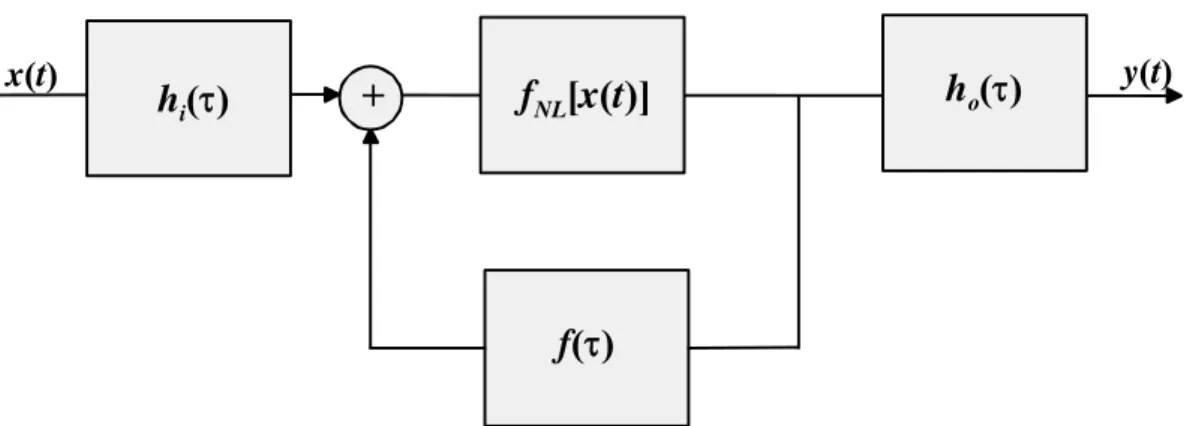
In some cases it can be observed a different type of dynamics in PAs: nonlinear memory effects. Those are memory effects that are only visible when the amplifier enters it’s nonlinear regime of operation. This type of effects can be modelled by a different topology as shown in Figure 2.3.

f

_NL

[x(t)]

f(τ)

x(t)

h_i(τ)

+

ho(τ) y(t)

Figure 2.3 – Schematic representation of a nonlinear amplifier with nonlinear memory proposed by Pedro et al.

Considering once again the Taylor series expansion of (2.7) for fNL[x(t)], the first and third order Volterra kernels of this system are [2.6,2.7]:

( )

( )

( )

ω

( )

ω α ω ω O D I H = ⋅ 1 ⋅ 1 (2.10a)

( ) ( ) ( )

( ) ( ) ( )

(

)

(

)

(

)

(

)

(

)

(

)

(

)

(

)

⎭⎬ ⎫ ⎩ ⎨ ⎧ ⎥ ⎦ ⎤ ⎢ ⎣ ⎡ + + + + + + + + + ⋅ + + + + = 3 2 3 2 3 1 3 1 2 1 2 1 2 2 3 3 2 1 3 2 1 3 2 1 3 2 1 3 2 1 3 3 2 ) , , ( ω ω ω ω ω ω ω ω ω ω ω ω α α ω ω ω ω ω ω ω ω ω ω ω ω ω ω ω D F D F D F D O D D D I I I H (2.10b) where D(ω) = 1 – α1F(ω).

Contrary to the Volterra descriptions of the last examples, in this equation the nonlinear dynamic effects are visible in the product of α22 by a rational of the feedback filter transfer function.

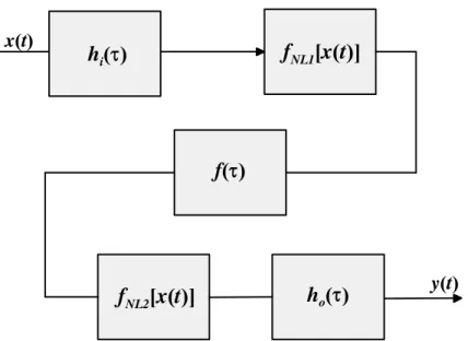
f

_NL1

[x(t)]

f(τ) x(t) hi(τ) y(t) ho(τ)

f

_NL2

[x(t)]

Figure 2.4 – Schematic representation of a nonlinear amplifier with nonlinear memory. proposed by Vuolevi et al.

In this model topology the nonlinear dynamic effects are modelled by the nonlinear mixtures of the dynamic response of the filter f(τ) that are created in fNL2[]. Note that since the filter f(τ) is placed after fNL1[] it processes baseband components created by the first nonlinearity that are then up converted by fNL2[].

If we assume that fNL1[] is equal to fNL2[], then this model topology is a simplified version of the one of Figure 2.3.

2.2.2 Different Behavioural Model Capabilities

In this section some illustrative examples of the more common behavioural model approaches are described. Different model examples are presented according to their capabilities of modelling the different phenomena presented in the last section.

Note that it is not the aim of this text to present an exhaustive description of all the behavioural modelling approaches. Given that they are so many, its description would go far beyond the scope of this thesis.

Memoryless Models

The models with the simpler structure are also the ones with less dynamic predictive capabilities – the memoryless models. The most commonly cited model of this kind is the complex polynomial series:

( )

_∑

−

( ) ( )

= + = 1 0 2 1 2 ~ ~ ~ N n n n x t x t a t y (2.11)

where x~(t) is the complex envelope input and a2n+1 are the complex coefficients used. It is seen in (2.11) that in this approach the output envelope y~( )t is dependent only on the present value of the input envelope, thus it is impossible to represent any memory effect with a model formulation like this one.

Another well known memoryless model is the Saleh model, [2.10] in which:

( )

[

]

( )

( )

[

]

2 1 r t t r t r r x r x r x y _β α + = (2.12) and

( )

[

]

( )

( )

[

]

2 1 r t t r t r x x x y φ φ β α φ + = (2.13)

where rx, φx, ry and φy are the amplitude and phase parts of the input and output complex envelope signals, respectively. αr, βr, αφ and βφ are parameters used to fit the modelled and measured transfer curves, from Amplitude Modulation to Amplitude Modulation (AM-AM) and from Amplitude Modulation to Phase Modulation (AM-PM). Despite this modelling approach intends to model amplitude and phase, both of them are once again only dependent on the instantaneous input complex envelope amplitude, and thus this model is considered a memoryless model.

Models of this type – memoryless – are well suited for modelling systems in which the input and output filters’ (hi(τ) and ho(τ) in Figure 2.3) bandwidth is considerably wider than the bandwidth of the signal processed by the system, so that those filters can be considered flat. Additionally, the feedback path filter f(τ) should also be flat so that the nonlinear mixing through the feedback path doesn’t create memory effects in the system.

Models addressing linear memory

When the signal’s bandwidth approaches the bandwidth of the system, then its response can no longer be considered flat – it presents linear memory effects. This way the memoryless models (extracted with a single CW excitation) are no longer valid approximators for these systems. Since the approximation problem appeared from the bandwidth increase, one of the proposed solutions was to consider AM-AM and AM-PM curves dependent on the input frequency. This was the approach of Saleh frequency dependent model [2.10] intended to be used on TWT amplifiers. Saleh proposed a new model formulation in which the complex envelope output amplitude and phase are dependent on the input complex envelope amplitude as previously, but also on the carrier frequency. This dependence of the AM-AM and AM-PM curves on the carrier frequency can be understood as the modelling of a linear filter connected in series with the previous frequency independent nonlinearity. To understand the impact of the input and output filters, let’s focus on the schemes of Figure 2.1 and Figure 2.2. In the memoryless case the output complex envelope can be written as:

( )

t f

[

x

( )

t

]

y _NL ~

~ _{= (2.14)}

If the effect of the input filter is now considered, in a configuration usually known as Wiener two box model, the complex output will be given by:

( )

t f

[

h

( )

t x

( )

t

]

y _{NL i} ~

~ _{= ∗ (2.15)}

The input filter can change the amplitude of the signal entering the nonlinear block, feeding the nonlinearity with different input power levels. Thus the AM-AM and AM-PM curves can be shifted horizontally (along the input power axis) by changing the coefficients of the input filter.

On the other hand if the effect of the output filter is considered separately, the two-box Hammerstein model is obtained. In this case the output complex envelope will be given by:

( )

t f

[

x

( )

t

]

h

( )

t y = _NL ~ ∗ _o

~ _(2.16)

From this expression it can be seen that the output filter impulse response ho(τ) is convolved with the nonlinearity output and thus can control the output amplitude. Thusthe output filter can shift the AM-AM and AM-PM curves vertically (along with the output power/output phase axis).

The reasoning above presented states that both configurations are essentially different, and thus cannot be interchanged. Actually, it is quite frequent the usage of both configurations simultaneously in a three box configuration: filter – memoryless nonlinearity – filter. This structure is also known as the Wiener-Hammerstein model.

One of the first published works using this topology was one work of Blachman in the 60’s [2.11]. In these earlier studies a framework was created for the study of nonlinear bandpass systems. Blachman identified each of the nonlinearity output autocorrelation function components: the signal X signal, the noise X noise and the signal X noise [2.12]. With these definitions, ways of identifying and separating the output signal from the output noise components were developed in order to characterize the signal quality degradation in the nonlinearity. Furthermore, studies ofthe interference impact of two signals of different amplitudes processed in the same PA were conducted [2.13].

Further examples of three-box models are the Poza-Sarkozy-Berger [2.14] and the Abuelma’atti models [2.15].

Different modelling approaches that also lead to models with these predicting capabilities are the ones based on polyspectral higher order statistics proposed by C. Silva et al. in [2.16]. In these works it is assumed that the nonlinear FIR filters can be represented by one-dimensional systems – which forces the systems to be represented by a two box model (either Wiener or Hammerstein configuration), in which the nonlinearity is the measured AM-AM and AM-PM curve. The main advantage of this approach is that it allows the model extraction with one CW test (to determine the AM-AM and AM-PM static curves) followed by an envelope test (to determine the cascaded filter). However this configuration is incapable of representing the systems’ nonlinear memory, as will be seen in the next sub-section. Other example of a three box model is the one proposed by Ibnkahla etal [2.17], that uses an ANN to approximate the three box structure.

Models Addressing Nonlinear Memory

Despite all the model formulations presented above, there are some types of effects that can not be modelled by any of the models already presented. For instance, an amplifier in which the output y~( )t depends, not only on the present value of the input complex envelope x~( )t , but also on its past values requires a different model structure.

Back in 2000, Fang et al. [2.18] proposed a recursive neural network model for a 1 GHz bandpass amplifier. Unfortunately the ANN was trained and tested with the same type of unmodulated data. This way the ANN training process can not capture any envelope dynamic effects since they were not excited by the training data. In this case the adopted extraction procedure (basically the excitation choice) does not allow taking full profit from the general predictive capabilities of the adopted ANN structure.

A different approach has been proposed by Mirri et al. [2.19] and further developed by Ngoya et al. [2.20] and Soury et al. [2.21]. This strategy consists in an application of the nonlinear integral model (NIM) of Filicori et al. [2.22] and is based on the assumption that the signal can be nonlinearly processed in the system in a static way while the dynamic effects introduced can be described in a linear way. In this strategy the systems’ response is expanded in a Taylor series around a predetermined nonlinear operating input x0(t) in the following way:

( )

_∑

[

( )

]

(

)

= − ⋅ ≈ Q q q q q t x t x f t y 1 0 ,τ τ (2.17)

this formulation can lead to the definition of a nonlinear impulse response, dependent on the static approximation point h[x0(t),τ]

( )

≈

_∫

∞

[

( )

]

⋅

(

−

)

0 0 t ,τ x t τ dτ x h t y . (2.18)

A different approach that also leads to a parallel Hammerstein topology was proposed by Ku [2.23]. Ku intended to model the memory effects shown by power amplifiers when excited by two tone RF signals. In that work the authors started with a usual AM-AM/AM-PM memoryless polynomial representation of the nonlinearity (similar to the one in (2.11)) and imposed coefficient dependency with frequency, obtaining, this

( )

_∑

−

( )

( )

( )

= + ⋅ ⋅ = 1 0 2 1 2 ~ ~ ~ N n n n x t x t a t y ω (2.19)

where ωm represents the frequency of the envelope sinusoid, which is the envelope equivalent of the particular two tone input.

A heuristic parametric approach has been proposed by Asbeck et al. [2.24] and continued by Draxler et al. [2.25]. The main idea of this approach was the extension of the AM-AM/AM-PM modulation by assuming that for an amplifier with long term memory effects its transfer characteristics will no longer be solely dependent on the instantaneous input envelope amplitude but also on a parameter that is a function of the envelope past inputs. If the PA transfer characteristic is represented by G which used to be considered as a function of rx(t): G

[

r_x

( )

t

]

; this work considers G as a function of the present input envelope and also of a parameter z~( )t dependent on the past input envelope samples:

( ) ( )

[

z t r t

]

G~ , _x . Then the authors expand G

[

~z

( ) ( )

t ,r_x t

]

by a first order Taylor series. This way the PA is modelled by a complex gain that is a nonlinear function of the instantaneous envelope amplitude and also of a parameter obtained by linear filtering of the input envelope past samples.

In a recent publication Dooley et al. [2.26] proposed a recursive model based on a IIR filter with a new approach for improving the coefficient determination of the structure. Starting with a vector of input and output data it was possible to develop an algorithm that uses the measured output sample at each process’ iteration for coefficient determination (and not the one computed with the estimated coefficients). This way the convergence and accuracy of the coefficient extraction are increased. The results obtained with this modelling strategy are compared with a conventional 3rd order VS model and a model approximation improvement was shown.

A more formal approach has been followed by Brazil and his group. In 2003 they have proposed a least square error extraction procedure for a hybrid time and frequency domain Volterra representation of a RF bandpass PA [2.27]. Despite nothing is said on the order of the model extracted nor on the number of time delays considered, the fact is that remarkably good results have been achieved with a model able to reproduce the variations in the third and even the fifth order Inter-Modulation Distortion (IMD). Recently, Zhu et al