A
W
ORKP
ROJECT,
PRESENTED AS PART OF THE REQUIREMENTS FOR THEA
WARD OF AM
ASTERD
EGREE INE
CONOMICS FROM THENOVA
S
CHOOL OFB
USINESS ANDE
CONOMICS.
OPTIMAL TAXATION AND INVESTMENT-SPECIFIC
TECHNOLOGICAL CHANGE
Valter Miguel Sobral Nóbrega
33080
A
P
ROJECT CARRIED OUT ON THEM
ASTER INE
CONOMICSP
ROGRAM,
UNDER THE SUPERVISION OF
:
OPTIMAL TAXATION AND INVESTMENT-SPECIFIC
TECHNOLOGICAL CHANGE
Valter Miguel Sobral Nóbrega
ABSTRACT
In this paper, we look at the relationship between Investment Specific Technological Change (ISTC) and optimal level of labor income progressivity. We develop an incomplete markets overlapping generations model that matches relevant features of the US economy and find that the observed drop in the relative price of investment since the 1980's leads optimal progressivity to increase. This result hinges on ISTC increasing the wage premium through an increase in the variance of the permanent component of labor income. This result is supported by recent findings in the literature that highlight the increasing role of the permanent component of labor income in the observed increase in income inequality. Keywords: Optimal taxation, Technological Change, Income Inequality
This work used infrastructure and resources funded by Fundação para a Ciência e a Tecnologia (UID/ECO/00124/2013, UID/ECO/00124/2019 and Social Sciences DataLab, Project 22209), POR Lisboa (LISBOA-01-0145-FEDER-007722 and Social Sciences DataLab, Project 22209) and POR Norte (Social Sciences DataLab, Project 22209).
1
Introduction
Optimal taxation theory tries to explain how a government can maximize the social welfare function using a fiscal system that considers consumption and saving allocations from households. The government may want to use taxation in order to correct efficiency or inequality problems in the society. For instance, it might want to use progressivity in order to reduce income inequality and insure low-income households from possible idiosyncratic productivity shocks. Nevertheless, it must consider the fact that this policy tool may also affect efficiency in the economy, and the result might not be coincident with its initial purpose.
It is true however that income inequality and progressivity have had different trends since 1980. Income inequality has sharply increased, and inversely, the relative price of investment decreased due to technological improvements. Investment-Specific Technological change theory suggests that these two phenomena are connected because capital is a substitute for routine jobs and a complement for non-routine jobs. The labor share has also declined due to the reduction of investment prices and therefore the wage premium has grown. Inequality started when relative demand for non-routine workers tended to increase, leading to unemployment in routine workers. This thesis tries to connect the influence of Taxation in shaping welfare with the increase in inequality due to Investment Specific Technological Change. It intends to simulate the influence of a drop on the relative investment price on the optimal taxation in 1980. This thesis uses a model with incomplete markets, overlapping generations, heterogeneous agents and partial uninsurable idiosyncratic risk. The distinguish factor of this model is the fact that it incorporates two different types of tasks as in Autor et al. (2003): routine jobs and non-routine jobs. The model is calibrated
to match the data of US economy in 1980 and subsequently the relative price of investment is changed to match the observed drop in the data between 1980 and 2010.
The model captures some important aspects of Optimal Taxation and Investment Specific Technological Change Theory: (i) optimal progressivity increases with the dispersion of permanent ability; (ii) skill heterogeneity always implies positive progressivity; (iii) higher wage premium and post-tax income Gini is associated with the drop on investment prices; (iv) routine labor share decreases due to its substitutability with capital, which is now less expensive.
The rest of the dissertation is as follows: in Section 2 we discuss some related literature; in Section 3, we describe the model and the calibration method and in Section 4 the results; section 5 concludes.
2
Literature Review
Ramsey (1927) was the first paper that contributed to analyze of Optimal Taxation, lacking, however, to incorporate heterogeneity across the population. This is a key feature for this thesis, taking for instance the findings of Huggett et al. (2011) according to which heterogeneity in initial conditions accounts for about 61.5% of the variation in lifetime earnings for the United States. Mirrlees (1971) introduced a way to mathematically analyze the problem of unobserved heterogeneity in which agents only differ in their abilities. In the Mirrlees’ approach, the government faces an imperfect information problem due to the trade-off created by unobserved heterogeneity, diminishing marginal utility of consumption and incentive effects. Thus, when government increases redistribution, it has to guarantee that the highest qualified workers continue to produce in the level corresponding to their capacity. According to this approach the government
diminishing marginal utility of consumption and incentive effects. Thus, when government increases redistribution, it must guarantee that the highest productive workers continue to produce in the level corresponding to their capacity.
There are two very important results introduced by Mirrlees (1971) that are fundamentals in this paper. First, that Optimal Taxation depends on the distribution of ability. It is, in fact, the schedule of marginal tax rates and how they are tailored to the shape of the ability distribution that defines the balance between equality and efficiency. One of his conclusions is that it would be optimal to have a zero marginal tax rate at the top, however several other studies differ in this point. For instance, Saez (2001) concluded that marginal tax rates should rise between middle-and high-income earners, and that rates at high high-incomes should “not be lower than 50% and may be as high as 80%”. Other authors have different conclusions, these diverse results are consequences of different theories of what makes a worker reach the top of the income scale.
The second important result from Mirrlees (1971) is that the optimal marginal tax rate rises with wage inequality due to a change in the distribution of ability, increasing the benevolent effects of redistribution. More recently other authors also connected the increase in inequality with a more redistributive tax system. Heathcote et al (2017) showed that tax progressivity increases with appropriate measures of inequality. Moreover, they show that it is the permanent component of the income process that is responsible for most of the increase in income inequality since the 1980s.
Krueger et al. (2009) stated that household heterogeneity and idiosyncratic earnings risk are key determinants of the progressivity of labor income taxes. Using a model with idiosyncratic uninsurable income shocks and permanent productivity differences across households they concluded that, since redistribution is insurance against low ability (the value function
is possible by using progressive labor income taxes or taxation of capital income, or both. This relation between wage inequality and the optimal tax system is the key element of this dissertation, connecting Optimal Taxation Theory with Investment-Specific Technological Change which tries to relate the increase in wage inequality through the decline of investment price goods.
For instance, the drop on investment prices can be partially explained by the improvement in computer performance: since manual computing, performance increased by a factor between 1.7 trillion and 76 trillion (Nordhaus 2007). Thus, during this period of automation improvement labor share also declined as showed in Karabarbounis and Neiman (2014) that, using a general equilibrium model to obtain an expression for the labor share as a function of the price of investment goods, concluded that this mechanism is able to explain half of the observed decline in the labor share.
There are many shreds of evidences that a positive correlation between the computerization of the workplace and skilled labor in production exists. Autor et al (2003) found out that computerization is associated with the reduction of routine labor and with the increase in non-routine jobs. They state that because of the decline of investment price, capital should have substantially substituted for workers performing routine unskilled tasks. Computer capital is then a substitute for cognitive and manual tasks that can be concluded following explicit rules and complements non-routine jobs characterized by problem-solving and complex communications tasks. Their model represents 60% of the change in the relative demand estimated in the last quarter of the twentieth’s century. Task changes within nominally identical occupations account for almost half of this impact. This thesis uses the same description of tasks as in Autor et al (2003), i.e., tasks are divided in routine (can be accomplished by machines following explicit programming rules) and non-routine (tasks for which
the rules are not sufficiently well understood to be specified in computer code and executed by machines).
Even though this dissertation uses a task framework as in Autor et al (2003), tasks and skills might be correlated: while investment price has declined, firms tended to substitute expensive labor for machines and it created significant advantages for workers whose skills become increasingly productive (Acemoglu and Autor, 2011). Acemoglu (2002) concluded that technical change has been skill-biased during the last century resulting from the rapid increase in the supply of skilled workers and the recent increase in inequality is probably a consequence of the acceleration in skill bias. Acemoglu and Autor (2011) also concluded that, after analyzing the effects of technology on the relative demand for skills, those effects are related with technology and in special to the skill bias of technical change. They also stated that automation creates negative effects on the real wages of the group that has been replaced.
Inequality is then created (i) when unemployment rates increase to unskilled workers due to the demand for clerical and information-processing tasks (non-routine) and (ii) when routine households’ wages decrease. These two consequences of SBTC result from capital-skill complementarity and are explained by Krussel et al. (2000). Automation increases the aggregate welfare by raising productivity and changing factor prices (Acemoglu and Restrepo, 2018), therefore if the stock of capital increases, marginal productivity of skilled labor increases but the opposite occurs for non-skilled workers. When adding the reduction of investment prices to this mechanism, the result is that firms will substitute away from labor towards capital. Krussel et al. (2000) estimated that the capital-skill complementarity effect increased the skill premium about 60 percent over the sample and the effect after 1980 is about 2.1 percent per year.
This dissertation will then be centered in the idea that the increase in income inequality is a consequence of a drop in investment prices and, due to SBTC, it increased the relative demand for non-routine workers and amplified the importance of the permanent component in the income process of the population by increasing the wage premium. Guerreiro et al. (2017) analyzed the impact of a fall in the automation price that could lead to a massive income inequality. They concluded that income inequality could be reduced by making the tax system more progressive. Ferreira (2019) also concluded that the effects from SBTC account for 42% of the overall increase in income inequality.
However, tax progressivity with the aim of mitigating income inequality might create a loss in efficiency and in its initial purpose. Government must trade-off this concern against the standard distortions that this policy tool imposes on labor supply and capital accumulation decisions. In one hand, progressivity offers both social insurance against labor market insurance and redistribution concerning initial conditions. First, it leads to more equality and more equal distribution of income, wealth, consumption and welfare. Second, in the absence of formal or informal private insurance markets against idiosyncratic uncertainty, progressivity provides a partial substitute for these missing markets and therefore may lead to less volatile household consumption over time (Conesa et al., 2006). But on the other hand, progressivity creates distortions in the labor supply and skill investment. A tax schedule with increasing marginal rates reduces both the returns to working more hours and the returns to acquiring human capital. Moreover, if the equilibrium skill premium responds to skill scarcity, a more progressive tax system, by depressing skill investment, may exacerbate inequality in pretax wages and undermine the original redistribution intent (Heathcote et al., 2017).
3
Model
This modelling framework builds on Bewley (2000) and incorporates also the assumptions from Aiyagari (1994) and Hugget (1993): an incomplete markets economy with overlapping generations of heterogeneous agents and partial uninsurable idiosyncratic risk that generates both income and wealth distributions. This approach is based on Brinca et al. (2016) and includes a bequest motive in the same philosophy as Brinca et al. (2019).
This different methodology includes two types of workers: non-routine (NR) and routine (R); and three final goods sectors in the economy: consumption goods, non-ICT capital, and an ICT capital sector (Eden and Gaggl, 2018). One main assumption in this model is to use the capital-skill complementarity from Krussel et. all (2000), but with these two types of workers.
Demographics
Time is discrete and the economy is populated by J-1 overlapping generations. A household starts to work at age 20 (represented by 𝑗 = 0) and retires at age 65 (𝑗 = 45). After retiring, the households face a positive age-dependent probability of death, 𝜋(𝑗). At age 𝑗 = 80 households die with probability one, 𝜋(80) = 1. Hence, 𝜔(𝑗) = 1 − 𝜋(𝑗) defines the age-dependent probability of surviving, and so, at any given period the mass of retired agents of age 𝑗 ≥ 45 is equal to Ω𝑗 = ∏𝑖=𝑗𝑖=45𝜔(𝑖). There are no annuity markets and therefore a fraction of households leaves unintended bequests, denoted by Γ, which are redistributed in a lump-sum method between the households that are currently alive. Additionally, retired households receive a retirement subsidy from the government, Ψ𝑡. In order to all group employment weights match the observed data, agents draw a permanent ability level 𝑎 from a uniform distribution with thresholds 𝑝𝑅 and 𝑝𝑁𝑅. This is used to
accommodate labor income inequality from other sources such as differences in gender and race composition of groups (Brinca et al., 2019).
Labor Income
In this framework, households differ across different factors such as permanent ability 𝑎, asset holdings, persistent idiosyncratic productivity shocks and four discount factors 𝛽 ∈ {𝛽1, 𝛽2, 𝛽3, 𝛽4}. The idiosyncratic productivity shock 𝑢 is assumed to follow an AR (1) process in the form of:
𝑢𝑖𝑡 = 𝜌𝑢𝑢𝑖𝑡−1+ 𝜀𝑖𝑡, 𝜀𝑖𝑡~𝑁(0, 𝜎𝜀2). (1) Hence, the defining equation of household 𝑖’s wage is given by:
𝑤𝑖𝑡(𝑗, 𝑎𝑖, 𝑢𝑖𝑡) = 𝑤𝑡𝑠𝑒𝛾1𝑗+𝛾2𝑗2+𝛾3𝑗3+𝑎𝑖+𝑢𝑖𝑡, (2)
where 𝛾1, 𝛾2 and 𝛾3 try to capture the age profile of wages which are calibrated directly from data (1980 or 2010) and 𝑤𝑡𝑠, 𝑠 ∈ 𝑆 ≡ {𝑁𝑅, 𝑅}, is the wage per efficiency unit of labor.
Moreover, there is a wage differential between the two types of workers that tries to capture the share of between-group inequality which does not result from the value of the wage premium as determined by relative productivities. The within-group earnings inequality is modelled by constructing a wage distribution within each group in order to match the inequality in the data.
Preferences
Working-age agents have to choose how much to work, 𝑛𝑡, how much to consume, 𝑐𝑡, and how much to save, 𝑘𝑡+1, to maximize their utility which is increasing in consumption and decreasing in work hours. It is defined as:
𝒰(𝑐𝑖𝑡, 𝑛𝑖𝑡) =𝑐𝑖𝑡1−𝜆
1−𝜆 − 𝜒 𝑛𝑖𝑡1+𝜂
where 𝜒 represents the disutility of work and 𝜂 is the Frisch labor elasticity. This CRRA utility representation is used to produce a utility concave function: from a certain point, there is no wealth effect due to an increase in consumption, and this formulation enables a balanced growth. Retired households also face one extra term which is related to the bequest that they leave for future generation:
𝐷(ℎ𝑖𝑡′) = 𝜑𝑙𝑜𝑔(ℎ𝑖𝑡′ ). (4)
Technology
Using the Brinca et al. (2019) approach, there are three competitive final goods sectors: consumption, non-ICT capital and ICT capital. In this model, a representative intermediate goods firm produces 𝑍𝑡𝑐+ 𝑍𝑡𝑠 + 𝑍𝑡𝑒 using a constant returns to scale technology in capital and labor inputs; it rents non-ICT capital at rate 𝑟𝑡𝑠, ICT capital at 𝑟
𝑡𝑒 and each labor variety at 𝑤𝑡𝑠, 𝑠 ∈ 𝑆; it chooses in each period capital and labor to maximize the its profits:
Π𝑡𝑧 = 𝑝𝑡𝑧𝑦𝑡− 𝑟𝑡𝑠𝐾𝑠𝑡− 𝑟𝑡𝑒𝐾𝑒𝑡− ∑𝑠∈𝑆𝑤𝑡𝑠𝑁𝑠𝑡, (5) subject to:
𝑦𝑡= 𝑍𝑡𝑐 + 𝑍𝑡𝑠+ 𝑍𝑡𝑒 = 𝐶𝑡+ 𝐺𝑡+ 𝑋𝑠𝑡+ 𝜉𝑡𝑋𝑒𝑡 = 𝑌𝑡. (6) where 𝑍𝑡 is the quantity of input z used in the production of the final (consumption (𝑐), non-ICT capital (𝑠) or ICT capital (𝑒)) good, 𝑝𝑡𝑧 is the price of intermediate goods (which is equal to the marginal cost of production due to perfect competition), 𝑋𝑒𝑡 is the ICT capital good and 𝜉𝑡 is the relative price of the equipment good and 𝜉𝑡 = 𝑝𝑡𝑒 𝑝
𝑡𝑐 ⁄ .
Hence, assuming that the production function of intermediate goods is Cobb-Douglas over non-ICT capital and CES (Eden and Gaggl, 2018) over the remaining inputs, the aggregate demand
𝑌𝑡 = 𝐹(. ) = 𝐴𝑡𝐺(. ) = 𝐴𝑡𝐾𝑠𝑡𝛼[∑ 𝜑𝑍𝑡 𝜎−1 𝜎 3 𝑖=1 + (1 − ∑ 𝜑 3 𝑖=1 ) 𝑁𝑅𝑡 𝜎−1 𝜎 ] 𝜎(1−𝛼) 𝜎−1 , (7) 𝑍𝑡 = [𝜙𝐾𝑒𝑡 𝜌−1 𝜌 + (1 − 𝜙1)𝑁𝑁𝑅𝑡 𝜌−1 𝜌 ] 𝜌 𝜌−1 ,
where 𝐴𝑡 is total factor productivity, 𝜑 is the share of the composite factor, 𝜙 is the share of the ICT capital in the composite, 𝜌 is the elasticity of substitution between ICT capital and the non-routine labor and 𝜎 represents the elasticity of substitution between the composite 𝑍𝑡 and routine labor. In order to ensure that there is complementarity between the two inputs in the composite, it is necessary that 𝜌 < 𝜎. Moreover, the reason why the production function is CES over ICT capital is that this restriction allows non-routine labor to interact with “routine inputs”, which can be produced by either routine labor or ICT capital (Eden and Gaggl, 2018).
As a result, the capital laws of motion in this model are:
𝐾𝑠𝑡+1 = (1 − 𝛿𝑠)𝐾𝑠𝑡+ 𝑋𝑠𝑡, (8)
𝐾𝑒𝑡+1= (1 − 𝛿𝑒)𝐾𝑒𝑡 + 𝑋𝑒𝑡, (9)
in which 𝛿𝑠 and 𝛿𝑒 are the non-ICT capital and ICT capital depreciation rates, respectively. Government
The social security system is responsible for financing the retired households with labor and firm taxes, 𝜏𝑠𝑠 and 𝜏̃𝑠𝑠, and with these revenues, it pays retirement benefits, Ψ𝑡. The government collects taxes on consumption (𝜏𝑐), capital (𝜏𝑘) and labor (𝜏𝑙). Although the government uses flat rates on 𝜏𝑐 and 𝜏𝑘, the labor tax function in this model is one of the distinguishing factors following a non-linear functional form as in Gouveia and Strauss (1994) and Benabou (2002):
𝑦𝑎 = 1 − 𝜃1𝑦−𝜃2, (10) where 𝜃1 represents the level of the tax schedule and 𝜃2 defines the progressivity of the tax. Additionally, 𝑦 and 𝑦𝑎 are the pre-tax labor income and the after-tax labor income, respectively. Hence, the government intends to finance public goods 𝐺𝑡, public debt interest expenses 𝑟𝑡𝐵𝑡 and other lump-sum transfers 𝑔𝑡 while preserving a balanced budget with the previous taxes. Thus, the government budget constraint is represented as follows:
𝑔𝑡( ∑ Ω𝑗 𝑗≥45 ) = 𝑇𝑡− 𝐺𝑡− 𝑟𝑡𝐵𝑡, (11) Ψ𝑡( ∑ Ω𝑗 𝑗≥45 ) = 𝑅𝑡𝑠𝑠, (12)
where 𝑅𝑡𝑠𝑠 is social security revenues and 𝑇
𝑡 is the other tax revenues.
Asset Structure
There are three assets in the economy: ICT capital, 𝑘𝑒, non-ICT capital, 𝑘𝑠, and government bonds, 𝑏. In order to guarantee the non-arbitrage condition, investing in ICT capital must have the same return as investing in bonds. Moreover, in this market there is no investment-specific technological change, then in the steady-state, the relative price of the equipment good is constant. Thus, equation (13) represents the return rate on the bond, equation (14) denotes the return rate on non-ICT capital, and equation (15) defines the state variable for the consumer:
1
𝜉[1 + (𝑟𝑒− 𝜉𝛿𝑒)(1 − 𝜏𝑘)] = 1 + (1 − 𝜏𝑘), (13) 1
𝜉[1 + (𝑟𝑒− 𝜉𝛿𝑒)(1 − 𝜏𝑘)] = 1 + (𝑟𝑠− 𝛿𝑠)(1 − 𝜏𝑘),
ℎ ≡ 𝜉𝑘𝑒+ 𝑏 + 𝑘𝑠. (15) Competitive Equilibrium
In a perfect competition economy, firm’s profit maximization implies that factor prices have to be equal to their marginal products.
𝑤𝑡𝑁𝑅𝐶 = Ξ 𝑡𝜑 [𝜙 ( 𝐾𝑒𝑡 𝑁𝑁𝑅𝑡) 𝜌−1 𝜌 + (1 − 𝜙)] 𝜎−𝜌 (𝜌−1)𝜎 [1 − 𝜙], (16) 𝑤𝑡𝑅𝑀 = Ξ 𝑡(1 − 𝜑) ( 𝑁𝑅𝑡 𝑁𝑁𝑅𝑡) −1𝜎 , (17) 𝑟𝑡𝑠 = A𝑡𝛼 [ 𝐾𝑒𝑡 𝑁𝑁𝑅𝑡] 𝛼−1 [ 𝜑 (𝜙 ( 𝐾𝑒𝑡 𝑁𝑁𝑅𝑡) 𝜌−1 𝜌 + (1 − 𝜙)) (𝜎−1)𝜌 (𝜌−1)𝜎 + (1 − 𝜑) (𝑁𝑅𝑡 𝑁𝑁𝑅𝑡) 𝜎−1 𝜎 ] 𝜎(1−𝛼) 𝜎−1 , (18) 𝑟𝑡𝑒 = Ξ𝑡 [ 𝜑 (𝜙 [ 𝐾𝑒𝑡 𝑁𝑁𝑅𝑡 ] 𝜌−1 𝜌 + (1 − 𝜙)) 𝜎−𝜌 (𝜌−1)𝜎 𝜙1[ 𝐾𝑒𝑡 𝑁𝑁𝑅𝑡 ] −𝜌1 ] , (19) where: Ξ𝑡 = A𝑡[ 𝐾𝑒𝑡 𝑁𝑁𝑅𝐶𝑡 ] 𝛼 [1 − 𝛼] [ 𝜑 (𝜙 ( 𝐾𝑒𝑡 𝑁𝑁𝑅𝑡) 𝜌−1 𝜌 + (1 − 𝜙)) (𝜎−1)𝜌 (𝜌−1)𝜎 + (1 − 𝜑) (𝑁𝑅𝑡 𝑁𝑁𝑅𝑡) 𝜎−1 𝜎 ] 1−𝜎𝛼 𝜎−1 . (20)
For certain given prices, policies, transfers, and initial conditions, a household with age 𝑗, asset position ℎ, discount factors 𝛽, permanent ability 𝑎, and a persistent idiosyncratic productivity shock 𝑢, maximizes his utility on any given period by choosing consumption 𝑐, work hours 𝑛, and future asset holding ℎ′. His problem can be formulated recursively as:
𝑉(𝑗, ℎ, 𝛽, 𝑎, 𝑢) = 𝑚𝑎𝑥𝑐,𝑛,ℎ′[𝑈(𝑐, 𝑛) + 𝛽𝐸𝑢′[𝑉(𝑗 + 1, ℎ ′, 𝛽, 𝑎, 𝑢′)]] (21) s.t.: 𝑐(1 + 𝜏𝑐) + 𝑞ℎ′= ℎ + 𝛤 + 𝑔 + 𝑌𝑁 𝑌𝑁= 𝑛𝑤(𝑗, 𝑎, 𝑢) 1 + 𝜏̃𝑠𝑠 (1 − 𝜏𝑠𝑠 − 𝜏𝑙[ 𝑛𝑤(𝑗, 𝑎, 𝑢) 1 + 𝜏̃𝑠𝑠 ]) 𝑛 ∈ [0,1], ℎ′≥ −ℎ, ℎ0 = 0, 𝑐 > 0.
The retired households face the same problem apart from having three different characteristics: age-dependent probability of dying 𝜋(𝑗), constant retirement benefits and the bequest motive 𝐷(ℎ′) as in Brinca et al. (2019). Thus, their problem is defined as
𝑉(𝑗, ℎ, 𝛽, 𝑎, 𝑢) = 𝑚𝑎𝑥 𝑐,ℎ′ [𝑈(𝑐, 𝑛) + 𝛽(1 − 𝜋(𝑗))[𝑉(𝑗 + 1, ℎ ′, 𝛽) + 𝜋(𝑗)𝐷(ℎ′)]] (22) s.t.: 𝑐(1 + 𝜏𝑐) + 𝑞ℎ′= ℎ + 𝛤 + 𝑔 + 𝛹 ℎ′ ≥ −ℎ, 𝑐 > 0.
The equilibrium in this framework is obtained by a stationary recursive approach, in which 𝛷(𝑗, ℎ, 𝛽, 𝑎, 𝑢) is the measure of agents that correspond to the characteristics (𝑗, ℎ, 𝛽, 𝑎, 𝑢). Hence, the stationary recursive competitive equilibrium is defined as in Brinca et al. (2019):
1. Taking factor prices and initial conditions as given, the value function 𝑉(𝑗, ℎ, 𝛽, 𝑎, 𝑢) and the policy functions, 𝑐(𝑗, ℎ, 𝛽, 𝑎, 𝑢), ℎ′(𝑗, ℎ, 𝛽, 𝑎, 𝑢), and 𝑛(𝑗, ℎ, 𝛽, 𝑎, 𝑢) solve the household’s optimization problem;
2. Markets clear: [𝜉 + (𝑟𝑒− 𝜉𝛿𝑒)(1 − 𝜏𝑘)] (𝐾𝑒+ 𝐵 𝜉 + 𝐾𝑠 𝜉) = ∫ ℎ + 𝛤𝑑𝛷 , (23) 𝑁𝑅 = ∫ 𝑛 𝑑𝛷 𝑎<𝑝𝑅 , 𝑁𝑁𝑅 = 𝜚𝑁𝑅∫ 𝑛 𝑑𝛷 𝑝𝑁𝑅𝑆≤𝑎 , 𝐶 + 𝐺 + 𝛿𝑠𝐾𝑠+ 𝜉𝛿𝑒𝐾𝑒 = 𝐹(𝐾𝑠, 𝐾𝑒, 𝑁𝑁𝑅, 𝑁𝑅) ; 3. Equations 16-19 hold;
4. The government budget balances: 𝑔∫ 𝑑𝛷 + 𝐺 + 𝑅𝐵 = ∫ (𝜏𝑘(𝑟𝑒∕ 𝜉 − 𝛿𝑒) ( ℎ + 𝛤 𝜉 + (𝑟𝑒∕ 𝜉 − 𝛿𝑒)(1 − 𝜏𝑘) ) + 𝜏𝑐𝑐 + 𝑛𝜏𝑙( 𝑛𝑤(𝑎, 𝑢, 𝑗) 1 + 𝜏̃𝑠𝑠 )) 𝑑𝛷 ; (24)
5. The social security system balances:
∫𝑗≥45𝛹𝑑𝛷 = 𝜏̃𝑠𝑠+𝜏𝑠𝑠
1+𝜏̃𝑠𝑠 (∫𝑗≥45𝑛𝑤𝑑𝛷) ; (25)
6. The assets of the deceased at the beginning of the period are uniformly distributed among the living:
𝛤 ∫ 𝑤(𝑗) 𝑑𝛷 = ∫(1 − 𝑤(𝑗))ℎ 𝑑𝛷 . (26)
The wage premia is endogenous and it can be expressed relative to routine wages as:
𝑤𝑁𝑅𝐶 𝑤𝑅𝑀 = [1 − 𝜙]𝜑 1 − 𝜑 [𝜙 ( 𝐾𝑒 𝑁𝑁𝑅) 𝜌−1 𝜌 + (1 − 𝜙)] 𝜎−𝜌 (𝜌−1)𝜎 [ℎ𝑅 ℎ𝑁𝑅] 1 𝜎 . (27)
4
Calibration
The calibration of the model is made to match the U.S. economy in 1980 as in Brinca et al. (2019). The parameters that are exogeneous are set directly to match the data. The endogenous parameters are estimated by using the simulated method of moments (SMM). Table 1 lists all values and sources of exogeneous parameters.
Preferences
Even though there has been a debate in the literature considering the parameter of Frisch elasticity, it is set to 1.0 as in Brinca et al. (2016). The parameter of risk aversion is also set to the same level.
Labor productivity
The wage profile that is defined in equation (2) is calibrated directly from the data. Equation (28) is run using data from the panel of Study of Income Dynamics (PSID):
ln(𝑤1) = ln(𝑤) + 𝛾1𝑗 + 𝛾2𝑗2+ 𝛾3𝑗3+ 𝜀𝑖 , (28) where 𝑗 is the age of individual 𝑖. The residuals of equation (28) are used to estimate the parameters governing the idiosyncratic shock 𝜌𝑢 and 𝜎𝜀. The wage differential between non-routine and routine groups is calibrated to match the log difference in average wages between groups in 1980. In order to see the employment level of the two groups, their values are set to equal their observed weight in total employment in 1980.
Technology
In this framework, both relative price of investment and total factor productivity are set to 1.0 in 1980. The production function parameters are the same as in Eden and Gaggl (2018).
The tax function used in this thesis is the same as in Gouveia and Strauss (1994) and Benabou (2002) (equation 10). The estimates of 𝜃1 and 𝜃2 in 1980 are from Ferriere and Navarro (2018). There is no progressivity for the social security rates, and both are set to 0.06, the average in 1980. Finally, the capital taxation 𝜏𝑘 and consumption tax 𝜏𝑐 are set to 0.47 and 0.05 respectively, in order to match the values obtained in Mendonza et al. (1994) for 1980.
Parameters calibrated using SMM
Given that there are several parameters that do not have any empirical counterpart, this framework uses the simulated method of moments so that the following loss function is minimized:
𝐿(𝜓, 𝛽1, 𝛽2, 𝛽3, 𝛽4, ℎ, 𝜒, 𝜎𝑁𝑅, 𝜎𝑅) = ‖𝑀𝑚− 𝑀𝑑‖ , (29) Since there are nine parameters, the model needs to have nine data moments to have an exactly identified system. Table 2 and Table 3 display the target data moments and the nine parameters, respectively.
Table 2: Calibration Fit
Data moment Description Source Target Model value
75-100/all Average wealth of households 75 and over
US Census
Bureau 1.31 1.30
𝑛̅ Fraction of hours worked PWT 0.33 0.33
K/Y Ratio between capital and
output BEA 3.0 3.0
var 𝑙𝑛 𝑤 NR; R Variance of the log wages CPS 0.23; 0.21 0.23; 0.21
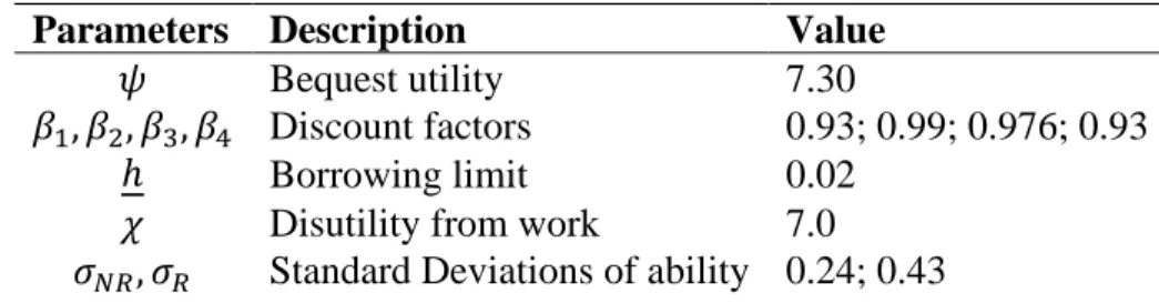
Table 3: Parameters Calibrated Endogenously
Parameters Description Value
𝜓 Bequest utility 7.30
𝛽1, 𝛽2, 𝛽3, 𝛽4 Discount factors 0.93; 0.99; 0.976; 0.93
ℎ Borrowing limit 0.02
𝜒 Disutility from work 7.0
5
Results
The most important mechanism of this thesis is from the drop of relative investment price. It is expected that with the decrease in investment prices, workers whose tasks are complementary to capital see their relative demand increase and therefore a higher equilibrium wage. Since workers get allocated to tasks at market entry depending on their ability level, the rise in the wage premium will increase the importance of the permanent component in their income process. Heathcote et al. (2017) show that this permanent component of the income process that is responsible for most of the increase in income inequality. If permanent component explains more of income dispersion, then optimal progressivity increases because it reduces consumption dispersion between different skills/tasks and increases insurance against low ability (Heathcote et al., 2017; Krueger et al., 2009). Hence, because this research changes the relative investment price, ceteris paribus, it is expected that the marginal benefits of progressivity are higher than their costs and optimal labor income progressivity will increase with respect to the benchmark economy in 1980.
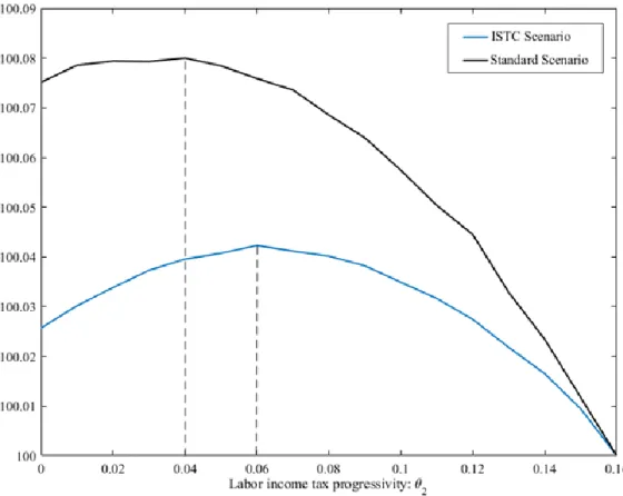
Figure 1 displays the levels of progressivity as a function of the Expected Social Welfare of an Unborn Individual. This is the parameter used to measure the changes in the social welfare because the social planner is utilitarian and, thus, he cares equally about the utility from consumption of all agents within a cohort. Then, according to Heatchote et al. (2017), the contribution to social welfare from any given cohort is the within-cohort average value for remaining expected lifetime utility. The Standard Scenario represents the benchmark model of 1980, and the ISTC Scenario is the same calibration, with the exception of the relative investment price which dropped from 1.0 to 0.586 in order to match the values in Brinca et al. (2019).
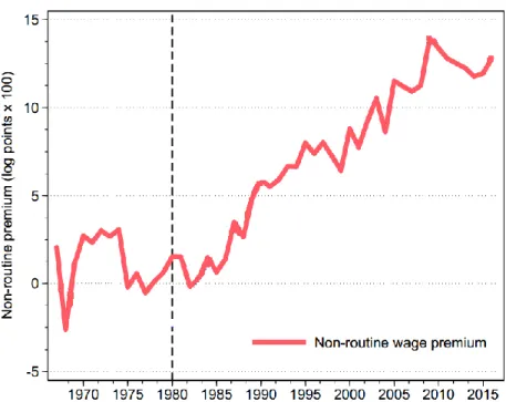
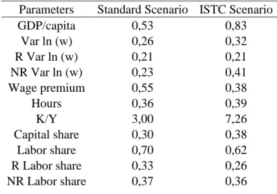
Figure 1: Horizontal axis: labor income tax function progressivity. Vertical axis: normalization of the changes of “Expected Social Welfare of an Unborn Individual” where the benchmark is 𝜃2= 0.16. The first result that can be understood when analyzing Figure 1 is that, in both cases, optimal labor tax progressivity is positive. Thus, this model captures the assumption from Heathcote et al. (2017): skill heterogeneity always implies positive progressivity. Moreover, ISTC increases the importance of redistribution, increasing optimal progressivity. The ISTC Scenario represents that mechanism: the drop on the relative investment price is responsible for an increase of 24% in the wage premium. This is a consequence of the observed change in the routine labor share that fell 23% due to the substitution effect between routine jobs and ICT capital that increased the capital share by 27%. These results are corroborated by Figure 2 from Brinca et al. (2019) where it is showed that the wage premium has increased since 1980.
Figure 2: The rise of non-routine wage premium (Brinca et al., 2019)
The rise in the wage premium will increase the importance of the permanent component in the income process of workers and thus, the optimal labor tax progressivity increased from 0.04 to 0.06. The comparative analysis is displayed in Table 4. In order to see an empirical example, using the tax function as in Ferreira (2019), if the average salary were 1000$, and it increased 50%, the average tax rate would change from 𝜏(𝑦) = 0,365 if 𝜃2∗ = 0,04 to 𝜏(𝑦) = 0,452 if 𝜃2∗ = 0,06.
6
Conclusions
Optimal taxation is one of the classic trade-offs in economy between efficiency and equality. It is helpful when a government wants to face inequality with fiscal policy, but it might be ineffective if the loss in productivity is higher than the gains of redistribution. Nevertheless, it may be a valuable fiscal tool to face a problem such as income inequality, which has increased in the last thirty years. This thesis uses a model with incomplete markets, overlapping generations,
technological environment there are two types of tasks that increase the dispersion of ability. Moreover, routine jobs are made substitute of capital in this model and conversely, the non-routine jobs are complement of capital.
The model is calibrated to match the data of US from 1980 and we try to capture the effects of the drop on the relative investment price in optimal progressivity, connecting Investment Specific Technological Change with Optimal Taxation. The most important result is the fact that optimal labor tax progressivity is not only positive but also increases with Investment Specific Technological Change. This experiment was also able to capture the increase in wage premium as well as the drop on the routine labor share, which are the main drivers to the increase in the optimal progressivity. This dissertation is able to demonstrate the link between the fall on relative investment price and the levels of optimal progressivity in the economy. All these effects are created in a model with different types of workers that respond differently to capital. These mechanisms may be important to predict future effects of automation that can start to become a substitute not only of routine but also of non-routine jobs through artificial intelligence, as in Acemoglu and Restrepo (2018).
A further study following this framework could examine how Investment Specific Technological Change accounts for the change in the optimal labor tax progressivity. Moreover, it would be interesting to study not only the impacts of the dispersion of ability, but also the effects of idiosyncratic productivity shocks that were eliminated in this model, adding this same analysis for the capital income tax and follow the works of Krueger et al. (2009).
References
Acemoglu, Daron, and David Autor. 2011. "Skills, tasks and technologies: Implications for employment and earnings." Handbook of labor economics. Vol. 4. Elsevier,. 1043-1171.
Acemoglu, Daron, and Pascual Restrepo. 2018. "Low-skill and high-skill automation." Journal of
Human Capital 12.2: 204-232.
Acemoglu, Daron. 2002. "Technical change, inequality, and the labor market." Journal of
economic literature 40.1: 7-72.
Aiyagari, S. Rao. 1994. "Uninsured idiosyncratic risk and aggregate saving." The Quarterly
Journal of Economics 109.3: 659-684.
Autor, David H., Frank Levy, and Richard J. Murnane. 2003. "The skill content of recent technological change: An empirical exploration." The Quarterly journal of economics 118.4: 1279-1333.
Benabou, Roland. 2002. "Tax and education policy in a heterogeneous‐agent economy: What levels of redistribution maximize growth and efficiency?." Econometrica 70.2: 481-517.
Bewley, T. F. 2000. “Has the Decline in the Price of Investment Increased Wealth Inequality?” Unpublished.
Brinca, P., Duarte, J. B., Holter, H. A., & Oliveira, J. G. (2019). Investment-Specific Technological Change, Taxation and Inequality in the US (No. 91960). University Library of Munich, Germany.
Brinca, P., Faria-e-Castro, M., Homem Ferreira, M., & Holter, H. 2019. “The nonlinear effects of fiscal policy”. FRB St. Louis Working Paper, (2019-15).
Brinca, P., Holter, H. A., Krusell, P., and Malafry, L. 2016. "Fiscal multipliers in the 21st century." Journal of Monetary Economics 77: 53-69.
Brinca, P., Homem Ferreira, M., Franco, F. A., Holter, H. A., and Malafry, L. 2018. "Fiscal consolidation programs and income inequality." Available at SSRN 3071357.
Conesa, Juan Carlos, and Dirk Krueger. 2006. "On the optimal progressivity of the income tax code." Journal of Monetary Economics 53.7: 1425-1450.
Conesa, Juan Carlos, Sagiri Kitao, and Dirk Krueger. 2009. "Taxing capital? Not a bad idea after all! “American Economic Review 99.1: 25-48.
Eden, Maya, and Paul Gaggl. 2018. “On the welfare implications of automation”. Review of
Economic Dynamics, 29.
Ferreira, A. M. 2019. “Skill-Biased Technological Change and Inequality in the US” (No. 93914). University Library of Munich, Germany.
Ferriere, Axelle, and Gaston Navarro. 2018. "The heterogeneous effects of government spending: It's all about taxes." FRB International Finance Discussion Paper 1237.
Gouveia, Miguel, and Robert P. Strauss. 1994. "Effective federal individual income tax functions: An exploratory empirical analysis." National Tax Journal: 317-339.
Heathcote, Jonathan, Kjetil Storesletten, and Giovanni L. Violante. 2017. "Optimal tax progressivity: An analytical framework." The Quarterly Journal of Economics 132.4: 1693-1754.
Huggett, Mark, Gustavo Ventura, and Amir Yaron. 2011. "Sources of lifetime inequality." American Economic Review 101.7: 2923-54.
Huggett, Mark. 1993. "The risk-free rate in heterogeneous-agent incomplete-insurance economies." Journal of economic Dynamics and Control 17.5-6: 953-969.
Karabarbounis, Loukas, and Brent Neiman. 2013. "The global decline of the labor share." The
Quarterly journal of economics 129.1: 61-103.
Krusell, P., Ohanian, L. E., Ríos‐Rull, J. V. and Violante, G. L. 2000. "Capital‐skill complementarity and inequality: A macroeconomic analysis." Econometrica 68.5: 1029-1053.
Mankiw, N. Gregory, Matthew Weinzierl, and Danny Yagan. 2009. "Optimal taxation in theory and practice." Journal of Economic Perspectives 23.4: 147-74.
Mendoza, Enrique G., Assaf Razin, and Linda L. Tesar. 1994. "Effective tax rates in
macroeconomics: Cross-country estimates of tax rates on factor incomes and
consumption." Journal of Monetary Economics 34.3: 297-323.
Mirrlees, James A. 1971. "An exploration in the theory of optimum income taxation." The review
of economic studies 38.2: 175-208.
Nordhaus, William D. 2007. "Two centuries of productivity growth in computing." The Journal of
Economic History 67.1: 128-159.
Ramsey, Frank P. 1927. "A Contribution to the Theory of Taxation." The Economic
Journal 37.145: 47-61.
Saez, Emmanuel. 2001. "Using elasticities to derive optimal income tax rates." The review of
A
Apendix
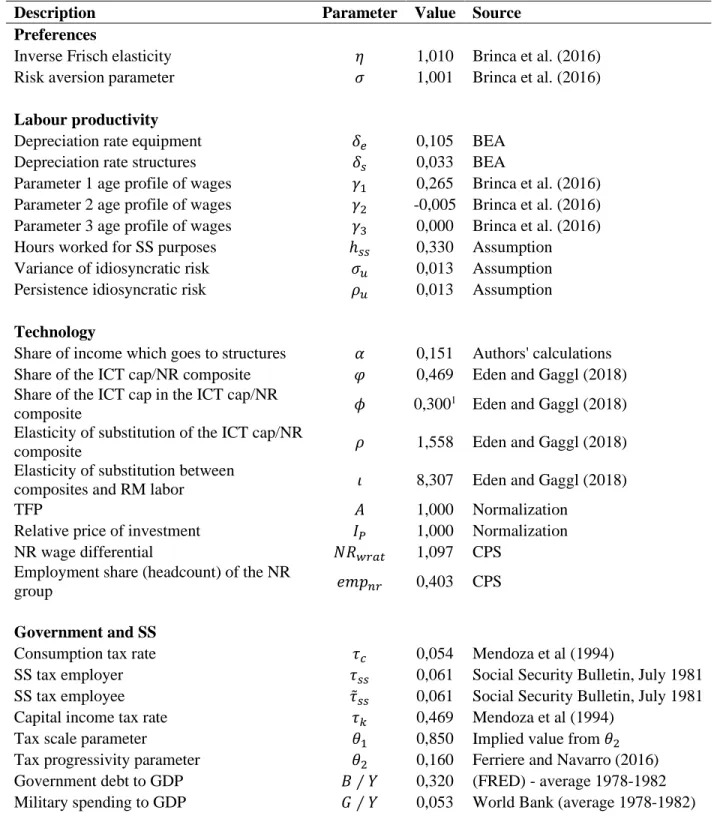
Table 1: 1980 Calibration Summary
Description Parameter Value Source
Preferences
Inverse Frisch elasticity 𝜂 1,010 Brinca et al. (2016) Risk aversion parameter 𝜎 1,001 Brinca et al. (2016)
Labour productivity
Depreciation rate equipment 𝛿𝑒 0,105 BEA
Depreciation rate structures 𝛿𝑠 0,033 BEA
Parameter 1 age profile of wages 𝛾1 0,265 Brinca et al. (2016) Parameter 2 age profile of wages 𝛾2 -0,005 Brinca et al. (2016) Parameter 3 age profile of wages 𝛾3 0,000 Brinca et al. (2016) Hours worked for SS purposes ℎ𝑠𝑠 0,330 Assumption Variance of idiosyncratic risk 𝜎𝑢 0,013 Assumption Persistence idiosyncratic risk 𝜌𝑢 0,013 Assumption
Technology
Share of income which goes to structures 𝛼 0,151 Authors' calculations Share of the ICT cap/NR composite 𝜑 0,469 Eden and Gaggl (2018) Share of the ICT cap in the ICT cap/NR
composite 𝜙 0,300
1 Eden and Gaggl (2018)
Elasticity of substitution of the ICT cap/NR
composite 𝜌 1,558 Eden and Gaggl (2018)
Elasticity of substitution between
composites and RM labor 𝜄 8,307 Eden and Gaggl (2018)
TFP 𝐴 1,000 Normalization
Relative price of investment 𝐼𝑃 1,000 Normalization
NR wage differential 𝑁𝑅𝑤𝑟𝑎𝑡 1,097 CPS
Employment share (headcount) of the NR
group 𝑒𝑚𝑝𝑛𝑟 0,403 CPS
Government and SS
Consumption tax rate 𝜏𝑐 0,054 Mendoza et al (1994)
SS tax employer 𝜏𝑠𝑠 0,061 Social Security Bulletin, July 1981 SS tax employee 𝜏̃𝑠𝑠 0,061 Social Security Bulletin, July 1981 Capital income tax rate 𝜏𝑘 0,469 Mendoza et al (1994)
Tax scale parameter 𝜃1 0,850 Implied value from 𝜃2
Tax progressivity parameter 𝜃2 0,160 Ferriere and Navarro (2016) Government debt to GDP 𝐵 ∕ 𝑌 0,320 (FRED) - average 1978-1982 Military spending to GDP 𝐺 ∕ 𝑌 0,053 World Bank (average 1978-1982)
Table 4: Results across scenarios
Parameters Standard Scenario ISTC Scenario
GDP/capita 0,53 0,83 Var ln (w) 0,26 0,32 R Var ln (w) 0,21 0,21 NR Var ln (w) 0,23 0,41 Wage premium 0,55 0,38 Hours 0,36 0,39 K/Y 3,00 7,26 Capital share 0,30 0,38 Labor share 0,70 0,62 R Labor share 0,33 0,26 NR Labor share 0,37 0,36
1. Average Tax Function
Using the same method as in Ferreira (2019), the average tax function 𝜏(𝑦) is obtained by: 𝑦𝑎 = 1 − 𝜃1𝑦−𝜃2
𝑦𝑎 = (1 − 𝜏(𝑦))𝑦