Maragro Group
Equity Valuation
Riccardo Biscontin
Dissertation written under the supervision of Prof. Josè Tudela Martins
Dissertation submitted in partial fulfilment of the requirements for the Msc in
Finance at Universidade Catòlica Portuguesa, 31.08.2018
Abstract
Title: Maragro Group Equity Valuation Author: Riccardo Biscontin
Keywords: Firm Valuation, Equity Valuation, Discounted Cash-flow, Adjusted Present Value
The aim of this dissertation is to estimate the fair value of the equity of Maragro Group, an enterprise located in Romania and operating in the Farming segment. The valuation has been performed by taking into consideration the latest financial information available as well as predictions made by the management team regarding the 2017-2018 campaign. For these reasons, the value of the company shall be intended as of the 31.12.2017. Methods used for the valuation include the discounted Cash-flow methodology and more specifically the Adjusted Present Value approach, whereas multiples have been taken into consideration as to analyze the possible differences that characterize the Group as opposed to the companies representing the peer group.
The outcome of this study is that Maragro Group shall be attributed a total enterprise value of 254.343.809 RON and an Equity value of 177.437.682 RON.
O objetivo desta dissertação é estimar o valor das ações do Grupo Marago, uma empresa localizada na Romênia que opera no setor agrícola. A avaliação foi realizada levando em consideração os últimos balanços financeiros assim como previsões realizadas pela equipe de gestão considerando os levantamentos de 2017-2018. Por essas razões, o valor da companhia será o estipulado em 31.12.2017. Os métodos usados para a avaliação incluem a metodologia do discounted Cash-flow e mais especificamente o valor presente ajustado, enquanto múltiplos fatores foram levados em consideração para analisar a possíveis diferenças que caracterizam o grupo como diferenciado dos demais. O resultado deste estudo é que ao Grupo Magoro deverá ser atribuído o valor total de 254.343.809RON e com valor de ação de 177.437.682 RON.
Executive Summary
Since its foundation in 2008, Maragro Group has witnessed an exponential growth in Revenue and especially in terms of EBITDA. With the introduction of the oil mill facility in 2015 and its full completion in 2017, the company is able not only to produce high-quality raw materials, but also to transform them into finished and semi-finished goods. The latest expansions as well as the introduction of organic farming, increased exponentially the margins of the Group, which is expected to reach full capacity in 2019 when 701 additional hectares will become available for farming. In light of the changes in structure and profitability that are expected until 2020, the Group shall be attributed a total value of 254.343.809 RON and an Equity value of 177.437.682 RON.
2015 2016 2017 2018E 2019E 2020E
EBITDA 8.392.444 RON 10.265.366 RON 12.418.427 RON 14.279.588 RON 17.880.504 RON 19.194.696 RON - RON 5.000.000 RON 10.000.000 RON 15.000.000 RON 20.000.000 RON 25.000.000 RON
Maragro Group
Acknowledgements
After two years at Catòlica Lisbon School of Business and Economics, my journey has come to an end. I can definitely state that, during this period, I have not only apprehended valuable skills that prepared me for my future career but that I have also grown as a person thanks to the prestigious environment and the people I had the opportunity to meet and to work with. I would like to thank in the first place my parents and more, in general, my whole family for the unconditional support they have provided me. If I have had the honour to attend a top-tier business school it is mostly thanks to them. I would moreover like to express my gratitude to all my colleagues, with which I worked and supported me during this experience. I strongly believe that the connections that have been established during this period will turn out to be a valuable asset also in future.
Gratitude goes also to the Casagrande Group, for which I have worked in the two years preceding my MSc in Finance and to the Maragro Group who has supported me in writing this dissertation.
As to conclude, I would also like to thank Prof. Tudela Martins for his support, the disponibility and patience he has shown in supervising the creation of this dissertation.
Table of Contents
1 Introduction ... 8 2 Valuation methods ... 9 2.1 Market Multiples ... 9 2.1.1 Multiples based on equity value ... 9 2.1.2 Multiples based on the company’s value ... 11 2.1.3 Relative multiples ... 12 2.2 Discounted-Cash-Flow methods ... 13 2.2.1 Cost of Equity, Cost of debt and WACC ... 15 2.2.2 Adjusted Present Value – Value Operations ... 17 2.2.3 Option Pricing, Decision Trees and Simulations – Value Opportunities ... 17 2.2.4 Terminal Value ... 18 2.3 Profitability methods ... 18 2.3.1 Dynamic ROE ... 18 2.3.2 Economic Value Added Method ... 19 2.4 Conclusion ... 20 3 Company profile ... 21 3.1 Timeline ... 21 3.2 Operativity ... 22 3.3 Group Structure ... 25 3.4 Financial Information ... 26 3.4.1 Shareholder composition ... 26 3.4.2 Debt composition ... 27 4 Industry Analysis ... 28 4.1 Geographical Setting ... 29 4.1.1 Exchange rate ... 30 4.1.2 Common Agricultural Policy (CAP) ... 32 4.2 Peer Group ... 33 4.3 Risk-free rate ... 34 5 Valuation ... 35 5.1 Valuation criteria ... 35 5.2 Defining the explicit period: Forecast of Revenue Streams ... 35 5.3 Defining the explicit period: Forecast of Operating Costs ... 405.5 Cost of Capital ... 43 5.6 Unlevered firm value ... 45 5.7 Effects of financing choices ... 46 5.8 Target Price and Scenario Analysis ... 48 6 Conclusion and Limitations ... 50 Bibliography ... 51 Annex I Historical Financial Statements ... 53 Maragro Group Income Statement (15-17) ... 53 Maragro Group Balance Sheet (15-17) ... 54 Annex II Revenue & Cost Forecast (explicit period) ... 55 Farming Revenue Forecast ... 55 Agrimeies Forecast ... 56 Farming Activity 2017 Campaign ... 57 Revenue Composition 2017 ... 57 Operating Costs Forecast ... 58 Depreciation of Fixed Assets Forecast ... 59 Annex III Financial Debt Composition ... 60 Annex IV Beta & Cost of Capital ... 61
Table of Contents: Tables
Tab. 1 Financial Stability ... 27Tab. 2 Source: Eurostat, Comex (16-18 Avg. Prices) ... 30
Tab. 4 Cultivation Outlook ... 36
Tab. 5 Forecast Production Farming ... 37
Tab. 6 Forecast Subsidies ... 39
Tab. 7 Subsidies Detailed ... 39
Tab. 8 Fixed Costs Frc. ... 40
Tab. 9 Source: European Parlament, Tradingeconomics ... 41
Tab. 10 Keyfigures Fin. Stability ... 42
Tab. 14 Terminal Value ... 46
Tab. 15 Calculation Tax Shield ... 47
Tab. 16 Scenario Analysis I ... 48
Tab. 17 Scenario Analysis 2 ... 49
Tab. 18 MV of Debt ... 49
Tab. 19 Target Price ... 50
Table of Contents: Figures
Fig. 1 Client Base ... 22Fig. 2 Revenue Composition ... 24
Fig. 3 Group Structure ... 25
Fig. 4 Shareholders ... 26
Fig. 5 EUR/RON Exchange Rate 2008 - 2018 ... 31
Fig. 6 GDP Growth Forecast ... 31
Fig. 7 10y. Yield on Rom. Government Bond ... 34
Fig. 8 Price Construction: Commodities ... 38
1 Introduction
“What’s it worth?”This sentence is not only the title of an article written by Professor Timothy A. Luehrman but is also a question that plenty of professionals face every time they have to evaluate whether or not to proceed with an investment on an asset.
When looking at the history of valuation methods, we can see how the focus of investors changed over time. According to (Rutterford, 2004), The first equity valuation techniques
used were dividend yield and book value, reflecting early investors’ perception of shares as quasi-bonds, differing only from bonds in the uncertainty of their maturity and of their dividend payments. In the same research paper named “from dividend yield to discounted cash flow: a history of UK and US equity valuation techniques”. The author also states that it took
the works of Smith (1925) and Fisher(1930) to get rid of this myth.
Nowadays barely a year goes by without a new model being launched (Young, Sullivan,
Nokhasteh, & Holt, 1999) witnessing the fact that there is no model that fits perfectly to all firms. In the following sections, I am going to list up the most popular valuation methods as of today and will then explain which ones I chose to perform the equity valuation of the group. As we will see there are models that are more appropriate for a company with a stable capital structure composition while others might be more indicated for a young company that has not yet reached the steady state and that might be subject to changes in the debt to equity ratio. And moreover, there are again other models appropriated to value a company performing in the financial sector.
As stated by (Luehrman, 1997b) whether the decision is to launch a new product, enter a
strategic partnership, invest in R&D, or build a new facility, how a company estimates value is a critical determinant of how it allocates resources. And the allocation of resources, in
turn, is a key driver of a company’s overall performance.
For these reasons selecting the right valuation method is a complex task of fundamental importance for the correct valuation of any business as well as defining the assumptions needed to properly apply the selected model. It shall be remembered that a valuation is only
2 Valuation methods
2.1 Market Multiples
These represent probably the most popular methods due to their ease of application. Starting from the assumption that an asset can be valued by means of the price of a similar asset that has been sold. This is usually done through a multiple that relates the value of the asset to a key parameter of the company.
According to (Fernandez, 2001) it is possible to identify three groups of multiples:
1.Multiples based on equity value
2. Multiples based on the company’s value (Debt+Equity) 3. Growth-referenced multiples
In the following sections, I am going to list the most common used multiples per each group.
2.1.1 Multiples based on equity value
2.1.1.1 PER – Price-Earnings ratio
This multiple is the most popular one among those based on the company’s capitalization. It relates the price per share to the actual earnings per share and can be represented as follows:
!"# =
!ℎ!"# !"#$%
!"#
Eq. 1where
2.1.1.2 P/CE – Price to Cash Earnings
! !" =
!"#$%! !"#$%"&$'"%$()
!"#$
Eq. 2where
EBDA = Earnings before depreciation and amortization
2.1.1.3 P/S – Price to sales
This multiple connects sales with share value only. It is a multiple used often to evaluate
companies performing in the internet and telecommunications sector as well as bus companies and pharmacies (Fernandez, 2001).
! ! =
!"#$% !"# !!!"#!!!"# !"#$%Eq. 3
2.1.1.4 P/BV – Price to book value
This multiple and its alternatives are used mainly to value companies in the financing sector such as banks but also insurance and real estate companies.
! !" =
!"#$%& !"#$%"&$'"%$()!" !" !"#$%&2.1.2 Multiples based on the company’s value
2.1.2.1 EV/EBITDA – Enterprise value to EBITDA
It is the most used multiple used to evaluate the value of a company. As opposed to the multiples based on equity value, this multiple, as well as the others that can be found in this subgroup use the sum of the firms market capitalization and financial debt. As stated by (Fernandez, 2001) the main limitation of this multiple is the fact that it ignores changes in
working capital requirements as well as capital investments.
!" !"#$%& = !"#$%&%'($ !"#$%
!"#$%$&' !"#$%" !"#$%$&#, !"#, !"#$"%&'(&)* !"# !"#$%&'!%&#( Eq. 5 2.1.2.2 EV/Sales - Enterprise value to sales !" !"#$%
=
!!"#$%$&'# !"#$% !"#$% Eq. 6 2.1.2.3 Enterprise value to unlevered free cash flow – EV/FCF!" !"! =
!"#$%&%'($ !"#$%
!"## !"#ℎ !"#$
Eq. 7 whereFree cash flow = Earnings before interest and after tax + depreciation + amortization – increased capital working requirements – capital expenditures
2.1.3 Relative multiples
These types of multiples are less used as they have to be contextualized. For the seek of completion I am going to list them anyway.
2.1.3.1 History-referenced multiple
!"#$%&' − !"#"!"$%"& !"#$%&#' =
!"#$%&#'
!"#$!%# !" !"#"$% !"#$%
Eq. 8This multiple is meant to compare the company’s recent performance with its own historical mean. Nevertheless, there are many limitations resulting from such an analysis as the historic
multiples depend on exogenous factors, such as interest rates and stock market situation
(Fernandez, 2001). In the same research paper, Fernandez argues also that the revenue composition and even the core business might change for firms over time, decreasing drastically the utility of such an analysis.
2.1.3.2 Market-referenced multiple
!"#$%& − !"#"!"$%"& !"#$%&#' =
!"#$ !"#$%&#'
!"#$%& !"#$%&#'
Eq. 9
An apparently much better analysis than the ones resulting from history-referenced multiples and market-referenced multiples. The limitations resulting from this method appear evident when the industry of interest is already subject to economic or market distortions. A good example is given by the financial bubble of 2008, whereas we can easily understand, the application of an industry-referenced multiple would have definitely led to a faulty valuation of firms performing in the housing industry.
In general, it has been proven that multiples nearly always have broad dispersion, which is
why valuations performed using multiples may be highly debatable. (Fernandez,2001). It is
often difficult to find an appropriate peer group as it is very unlikely to find a sister company in the market, that has already been evaluated. The concept of similarity in the business world is per se difficult to define limiting the objectivity of a valuation using multiples.
Nevertheless, it may be possible to rely on them at a later stage of the valuation, as a comparison between the firm that is being valued and the peer group might highlight differences among them which can be consequently further analysed.
2.2 Discounted-Cash-Flow methods
The Theory of Investment value is the title of a thesis published in 1938 by Williams in which
he defines the investment value, or the intrinsic value of a firm to be the present worth of
future dividends, of practical importance to every investor because it is the critical value above which he cannot go on buying or holding, without adding risk (Williams, 1938).
This concept is best proposed in the area of firm valuation by the Discounted-Cash-Flow methods.
Discounted Cash Flow Model (DCF)
!" =
!(!"
!)
(1 + !"##)
!!!!
!!! Eq. 11
where
EV= Enterprise value
E(!"!)= Expected Cash Flows at time t
WACC = Weighted average cost of capital
The DCF model values an enterprise by summing up all the future (expected) Cash-flows, discounted at the Weighted average cost of capital.
It is of major importance to understand the latter perfectly as a mistake in calculating the WACC can cause a relevant distortion in the valuation. (Fernandez, 2010) states in his paper
WACC: definition, misconceptions and errors, that it is neither a cost nor a required return: it is a weighted average of a cost and a required return. In the same paper he proposes the
following definition:
!"##
!=
!
!!!!"
!+ !
!!!!"
!(1 − !)
!
!!!+ !
!!! Eq. 12 where E!!! = PV!(Ke!; ECF!) T = Effective tax rate D!!!= PV!(Kd!; CFd!)It shall be noted that from these definitions it appears how in order to calculate the value of the company we need to discount the expected free cash flows to the firms at the WACC while to obtain the WACC we need to have in mind the value of the company.
Among the major limitations attributed to the WACC based DCF model is that, especially when the capital structure of the analyzed company starts to become more complex in the explicit time period, the valuation tends to misestimate the value of the company. This because it fails to analyze separately the risks or the opportunities that might be associated, among others, with hedges, subsidies, exotic debt securities and expansion possibilities. As stated by (Luehrman, 1997) the more complicated a company’s capital structure, tax
2.2.1 Cost of Equity, Cost of debt and WACC
The second step of a valuation based on discounted Cash-Flows, after the expected Cash Flows have been estimated, is to find the appropriate rates at which the former will be discounted.
The cost of equity shall be intended as the required rate of return that investors require to bear the cost of the risk associated with an asset. Most commonly accepted definition is provided by the Capital Asset Pricing Model (CAPM):
!" = !" + !" − !" × !
Eq. 13 where Ke = cost of equity rf = risk-free rate rm-rf = market premiumβ = idiosyncratic risk of the company
The cost of equity tends to increase as the leverage increases. This because a higher leverage leads to an increase in risk associated with the asset, thus the market premium (rm- rf) will be higher. Modigliani-Miller proposition II depicts this relationship with the following formula:
!" = !"
!+ (!"
!− !") ×
!
!
Eq. 14where
Ke = Cost of equity
!"! = Cost of equity of an unlevered firm
Kd = Cost of debt
!
The idiosyncratic risk measured by the beta in equation (13) measures the directly associated with the specific asset, in our case the Maragro Group. We can expect this value to be low as compared to companies of the same size performing in other industries as the degree to which
a product’s purchase is discretionary will affect the beta of the firm manufacturing the product (Damodaran, 1999). As the group is situated in the agricultural sector we can expect
this to have a positive impact on the riskiness of the asset.
As for the cost of debt, it shall be noted that the appropriate value to attribute to debt is the market value rather than the book value. This because many companies own debt that is not traded publicly (e.g. bonds) but can be mostly defined as non-traded such as bank loans. In order to provide the right valuation of debt, we shall take into consideration similar companies that have their debt traded. It might be even better to assign a credit rating to the company if this is possible.
The cost of debt is given by the weighted average internal rates of return of the different types of debt (e.g. bank loans, bonds, leasing) which are subordinated to the credit rating of the company to be valued. For most companies, with the exception of firms benefiting from a tax exemption, this should be estimated on an after-tax (1-t) basis.
Recent literature has nevertheless criticized the DCF method as, today the WACC-based
standard is obsolete (Luehrman, 1997). This because, the three dimensions on which a
complete valuation should be performed i.e. the valuation of operations, the valuation of opportunities and the valuation of ownership claims are summed up and discounted with a unique method in the classical DCF approach. Most experts agree that by using three different (complimentary) methods we should be able to outperform WACC-based DCF.
2.2.2 Adjusted Present Value – Value Operations
In order to assess the value of the operational part of the business recent literature suggests the Adjusted Present Value method or APV.
The theory behind this methodology is based on the philosophy of shared by the discounted cash flow methods. As stated by (Luehrman, 1997), the procedure is first to forecast the
expected future cash flows, period by period; and second, to discount the forecasts to present value at the opportunity cost of the funds.
The opportunity cost is the return a company (or it’s owners) could expect on alternative investments entailing the same risk.
As opposed to the more classical WACC method, APV relies on the concept of value additivity. By applying this principle we agree on splitting the forecasted cash flow as to analyze separately the different sources.
The method firstly discounts the expected cash flows as if the entity was unleveraged i.e. capital consists entirely of equity. In a second stage, the value of all financing choices is added which include positive effects as for example interest tax shields as well as negative effects such as financial distress costs.
This method is considered superior to the WACC method as it requires fewer restrictive
assumptions (Luehrman, 1997). It is thus less subject to massive errors.
2.2.3 Option Pricing, Decision Trees and Simulations – Value Opportunities
The opportunity to expand or to reduce a business, allows a business to be more likely to capture a larger market share as well as being less subject to financial distress. This flexibility is valuable and the problem of expressing this value in numbers is likely to be addressed by most professionals with the Option pricing method.
The said method compares, for example, a possibility to expand to an option.
As stated by (Luehrman, 1997), the potential investment to be made corresponds to an
option’s exercise price. The operating assets the company would own, assuming it made the investment, are like the stock one would own after exercising a call option. The length of time the company can wait before it has to decide is like the call option’s time to expiration.
In order to assess the risk for this option, we take into consideration the variance of the returns provided by said assets.
Based on the opportunity to evaluate it might be also useful to consider other methods such as decision trees or by relying on a simulation of various scenario analyses.
2.2.4 Terminal Value
The expected future cash flows should be predicted as to include the whole lifecycle of revenue growth. As the company approaches a steady state it is inevitable to assign a terminal value to the company. To do this we rely on the Gordon growth model, stating that for a company approaching the steady state it is reasonable to assume a constant growth of the dividends. By applying this theory to the valuation of a company we can express this mathematically as follows:
!" =
!"!!(1 + !)
!"## − !
Eq. 15 Where, g = Profit growthFCFF = Free cash flows of the last year of the explicit period
2.3 Profitability methods
2.3.1 Dynamic ROE
The Dynamic ROE method focuses on the concept of excess return (Damodaran, 2006) to equity rather than to total assets.
The value of the investment for a shareholder or a holding company can be summarized as follows:
!"#$%& !"#$% = !"# +
!"# − !" × !"#
!" − !
Eq. 16
Where,
g = Profit growth
EBV = Equity book-value ROE = Return on equity Ke = cost of equity
2.3.2 Economic Value Added Method
Said method is also known as economic profit method as it is aimed at capturing the real profit of a company by subtracting the cost of the funds involved. As stated by (Stewart; 1991) EVA is a measure of the true financial performance of a company.
The formula that captures said return is:
!"# = !"#$ − !"## × !"#$%"& !"#$%&$'
Eq. 17(2.17)
Where,
ROIC = Return on Invested Capital
which can be also expressed as:
!"#$% − !"##×!"#$%"& !"#$%&$'
Where,
As stated by (Damodaran, 2006), the Enterprise value of the company is the sum of the
expected future growth either of the assets in place and also of future projects.
!" = !"# !""#$" ×
!"#
!"## − !
Eq. 18 Where, g = Profit growth2.4 Conclusion
Virtually every popular valuation approach is simply a different way of expressing the same underlying model (Young et al., 1999).
According to this statement, it should follow that, in theory, all models are equally good at evaluating a company. Differences between one model and the others are simply the result of discrepancies in the underlying assumptions.
That being said while performing a valuation, different circumstances such as the availability of information regarding not only the company but also the industry and in general, the market the company is operating in can lead an analyst to prefer one model over another. As a general advice, in order to provide an objective valuation, one should try to minimize the assumptions to be done, as to decrease the impact of information asymmetries and to limit evaluation mistakes.
3 Company profile
Maragro is a company founded in 2008, which, either through direct ownership or through third parties, performs one of the most important agricultural farming, stocking and trading businesses in Western Romania, more precisely in the TIMIS region.
Maragro Group has started investing in the agricultural business in 2008. As for the agricultural year 2017-2018, its activities include 5135 ha of prime cultivated land representing a huge growth as compared to the 746 ha cultivated in 2009. Of this land, 4797 ha are either owned or rented while work is performed on a variable number of Ha for third parties. The Group has also been developed in order to include a 56.100 tons stockage centre built on 34.230m2 of the total surface. This centre can receive more than 120 trucks a day thanks to the high pumping capacity of the machines.
Maragro Group can be considered to be among the top farming activities in West-Romania, both because of its size and in relation to the completeness of its business. In fact, the Group’s operations cover all areas that constitute the primary sector of the agricultural production. Currently, Maragro cultivates land either directly or for third parties, produces seeds, stocks and dries up cereals and trades products for agriculture. The current farm is the result of 9 years of strong development, with a considerable work carried out to build new infrastructures able to manage an increasing amount of cultivated land and product.
The purpose of this development plan was to become also a service company, a stocking centre for other smaller regional farms granting a dynamic company structure able to offset a shortage of one of its sectors with an increase in another activity as to reach full capacity even in different scenarios.
3.1 Timeline
2008 Original Investment: A group of Italian Private Investors founds Maragro Srl and signs its first rental contract for 760 ha in Giera starting the activities only relying on services provided by third parties.
2009 The first tractors are bought, thanks also to the European Structural Funds, and the acquisition of a stocking centre from Comcereal Group is finalized. In the same year, Agrimeies Srl is founded.
2010 The implementation of the agricultural sector is completed, with the acquisition of modern and reliable equipment (Caterpillar, Claas, John Deere). The company is now able to perform also services for third parties.
2011 Rebuilding and expansion of the stocking centre is initiated. The company currently operates on 4900 ha of agricultural land.
2014 The expansion of the stocking centre is completed. In the same year, the works for the oil mill and the administrative building are initiated.
2015 The Oil mill structure, as well as the administrative building, are completed. A new warehouse has been built with the aim to increase the stocking capacity of finished products. 2016 The oil mill structure has reached full capacity now. The farming/cultivation segment increases its capacity with the acquisition of Agro Blochberger Srl, where it starts cultivating biological products. The acquisition will be finalized in 2018, after two years of rent.
2017 Production of biological goods is implemented with the conversion of agricultural land from the conventional method to the biological one.
3.2 Operativity
The Maragro Group sells its products mostly to top European players active both in the conventional and in the organic market. Approximately 90% of the client base is bound through a contract whose terms are negotiated, usually on a half-yearly basis. The usual payment terms are set at 30 days for raw materials and to 120 days for semi-finished goods. A snapshot of the client portfolio representing the major players is represented below in figure (1).
In contracting for the price of the goods to be supplied, Maragro Group takes into consideration the current market prices of the major agricultural exchanges. Among these the markets of the CME Group (e.g. CBOT), AGER Bologna, Associazione Granaria di Milano, Euronext Paris.
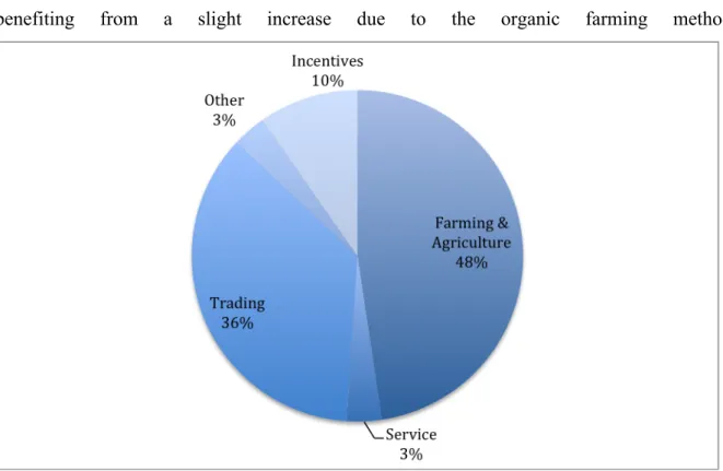
The Revenue of Maragro Group is built through five sources, namely the Farming and Seed Production segment, the oil mill segment (Agrimeies Srl), the trading segment, the service and stocking centre segment and finally through subsidies and incentives from the government. As for 2017, Maragro witnessed a slight decrease in the volumes generated by the farming and seed production sector. This was due to the bad weather conditions that characterized the year affecting negatively the yield per hectare. Nevertheless, the margins have been improved due to the transition to organic cultivation. Agrimeies saw its oil mill completed and full capacity has been reached, the benefits that come with economies of scale have been nevertheless limited by the decrease in price for vegetable oil combined to the slight increase of raw material cost. The strategy towards which the management team is oriented sees a reduction in the trading activity due to its low margins.
We see in this sense already an effect in revenue composition of 2017, where the stocking capacity of the group has been dedicated to a higher amount to the service segment as compared to the previous years. This shift in strategy will continue also in 2018 where it should stabilize around 5% of total income and should include only goods and fertilizers granting a high margin.
Finally, subsidies and incentives are in line with the level of production of the previous year, benefiting from a slight increase due to the organic farming method.
Fig. 2 Revenue Composition
Due to the pursue of more profitability in exchange for sales volume, the group achieved an increase in the relationship EBITDA/Total Sales of 5% as compared to the previous year, accounting now for 15% or 12.418.427 RON.
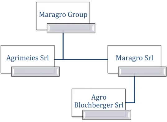
3.3 Group Structure
The group structure of the Maragro Group is represented by Figure (3).
Agrimeies Srl is operating mainly as an oil mill facility, while Maragro Srl is responsible for the cultivation of land, third party services and the trading activity. Agro Blochberger Srl is a subsidiary of Maragro Srl and is, as of 31.12.2017, entirely dedicated to the cultivation of biological products.
Fig. 3 Group Structure
Maragro Group
Agrimeies Srl
Maragro Srl
Agro
3.4 Financial Information
3.4.1 Shareholder composition
The composition and ownership is illustrated in fig. (4).
I.E.S. International Equipment Service, the main shareholder is an Italian holding company that controls several businesses in the industry
of drilling equipment, & in the real estate sector. It is a vehicle owned by the Casagrande family
META SRL is a company owned by two Italian entrepreneurs with several years of experience in the real estate industry. They moreover hold investments in the sector of gastronomy. Thanks to their contribution Maragro has not only been able to create a functional facility but to enrich it with details that are constantly appreciated.
Marco Chiaradia is an Italian entrepreneur with an academic knowledge of agriculture. Several years of experience in the sector building know how that has been transmitted to the company which has gained benefits not on the technical as in the commercial field. He is an expert of the international agro-business and of the fluctuations related to the agricultural commodities market. He is currently also investing in farming as well as building land in Italy.
Marco Chiaradia, 25%
I.E.S, 45% Meta S.r.l, 30%
3.4.2 Debt composition
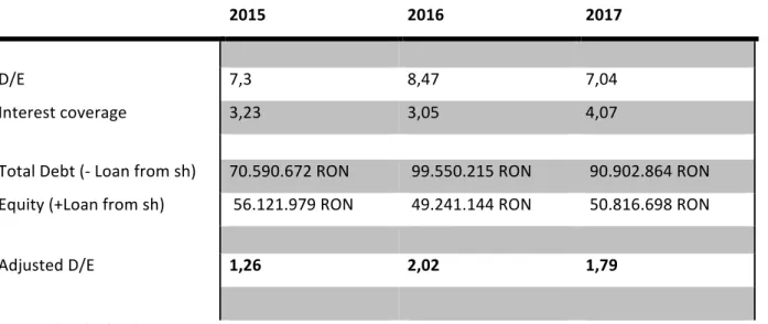
Financial debt composition of Maragro group is subject to two broad categories i.e. debt towards financial institutions and debt towards shareholders. How to treat the latter for valuation purposes has been a major challenge. On one side it will be treated as debt in evaluating the tax shield as interest expense deriving from it is tax deductible. As for the evaluation of the riskiness of the company, it will be considered as equity as no fixed terms for the repayment of the principal are defined, thus it will be only repaid in case of positive cash flows. Table (1) shows the evolution of (total) debt as compared to equity, while the whole balance sheets can be consulted in Annex (I). The voice adjusted D/E shows the debt to equity ratio if debt towards shareholders is treated as Equity.
2015 2016 2017
D/E 7,3 8,47 7,04
Interest coverage 3,23 3,05 4,07
Total Debt (- Loan from sh) 70.590.672 RON 99.550.215 RON 90.902.864 RON
Equity (+Loan from sh) 56.121.979 RON 49.241.144 RON 50.816.698 RON
Adjusted D/E 1,26 2,02 1,79
4 Industry Analysis
By 2050 the world population is estimated to increase to almost 10 million individuals. Various governments are faced with the challenge to feed these people and must rely on the agricultural sector to do so. This is the reason for which the latter has gained a major focus from authorities, as well as investors, in the recent years. Maragro Group is based in Romania but the revenue is in a large amount generated through exports to countries part of the European Union.
For this reason, the industry analysis has to be done in consideration of the huge impact of macroeconomic factors on the local, as well as in the European market.
Talking on a global level, the increment in population will contribute to the increase in demand for crop and food production. It shall be noted that, in this sense, more and more attention from the consumer side is expected with regards to the quality of food and it’s environmental and social impact. A study conducted in 2010 (Francisco et al.) has shown a relationship between consumers’ levels of knowledge and consumption of organic foods and has demonstrated that there is a willingness from the consumer to pay a premium for biological products. For the period 2017-2022 recent market researches predict a growth of the organic food market of roughly 16% on a CAGR basis.
Declining levels of yield gain rise concern on the supply side. As stated in the article Yield Trends Are Insufficient to Double Global Crop Production by 2050 (Ray, Mueller, West, & Foley, 2013).
Numerous studies have shown that feeding a more populated and more prosperous world will roughly require a doubling of agricultural production by 2050 [1]–[7], translating to a
∼2.4% rate of crop production growth per year. We find that the top four global crops –
maize, rice, wheat, and soybean – are currently witnessing average yield improvements only between 0.9 to 1.6 per cent per year, far slower than the required rates to double their production by 2050 solely from yield gains.
with countries such as Canada and Russia benefiting from the combined impact of increased temperatures, greater precipitation and the carbon fertilization effect. Meanwhile, countries closer to the equator, such as India and Africa, could be hit the worst as higher temperatures reduce crop yields.
The expectations for the European Agricultural Market given by the European Union predict a decrease of the utilised agricultural area to 172 million Ha by 2030. For the same period, cereal stocks will stabilise below historical levels, with common wheat expected to recover to above EUR 170/t until approaching EUR 194/t in 2030.
It is likely to see a reduction in rapeseed oil production, as the demand from the energy market for this product is decreasing. Soybeans will see an increase in demand given the high trend protein meals is experiencing while for sunflower oil production is expected to recover from the recent historically low margins.
4.1 Geographical Setting
Timisoara, which is also the best Romanian city for business according to Forbes (2016). The land in Giera is generally speaking from glacial origin, fairly homogeneous and extremely deep. The superficial layer measures approximately 1,5-2 meters. The mixture of the soil is between clay and slit (clay 40%, slit 40%, sand 20%). It is characterized by a fair level of organic substances (from 2,5 to 3,5 ppm) and phosphorus (from 15 to 40 ppm); it is very rich in potassium (from 150 to 240 ppm), magnesium (from 500 to 1000 ppm) and maintains an average level of nitrogen (1,4 – 1,6 g/kg).
The management team, based on these characteristics, estimates a potential yield of 5 T/Ha of wheat, 6 T/Ha of grain, 3 T/Ha of rape and 2,7 T/Ha of sunflower.
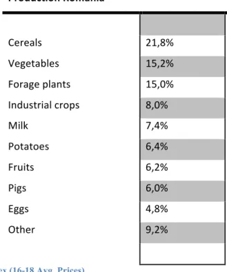
Production Romania Cereals 21,8% Vegetables 15,2% Forage plants 15,0% Industrial crops 8,0% Milk 7,4% Potatoes 6,4% Fruits 6,2% Pigs 6,0% Eggs 4,8% Other 9,2%
Tab. 2 Source: Eurostat, Comex (16-18 Avg. Prices)
4.1.1 Exchange rate
The Romanian Leu is expected to be replaced by the EUR in 2022, as stated by the Romanian Minister of foreign affairs Teodor Viorel Meleșcanu. In order to do so, among others, the Exchange rate stability parameter has to be respected.
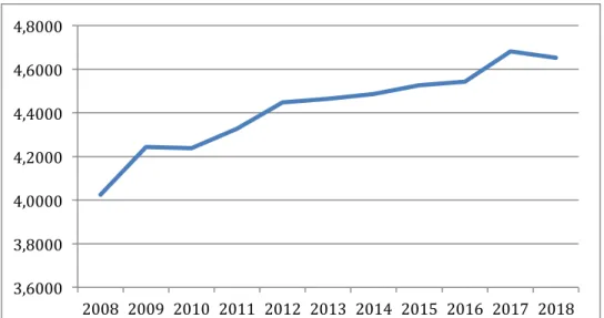
The ERM II provides the framework for entering the EUR and must be respected for a period of two years before entering the European currency. Generally speaking, the European Central Bank agrees with the central bank of the interested country on an exchange rate from which the local currency as compared to the EUR shall not fluctuate more than 15% on a yearly basis. As of the 31.12.2017 one EUR paid 4.6772 LEU, price which according to most analysts should remain stable during 2019.
Fig. 5 EUR/RON Exchange Rate 2008 - 2018 Source: Reuters
Fig. 6 GDP Growth Forecast Source: Statista
3,6000 3,8000 4,0000 4,2000 4,4000 4,6000 4,8000 2008 2009 2010 2011 2012 2013 2014 2015 2016 2017 2018 2,34 2,08 1,84 1,82 1,73 2017 2018 2019 2020 2021 % G RO W T H
4.1.2 Common Agricultural Policy (CAP)
Since 1962 the Common Agricultural Policy, or CAP, is the answer of the European Union to the challenging task of feeding an increasing amount of population while protecting local producers.
As of today, the European Agricultural Guarantee Fund and the European
Fund for Rural Development grant roughly €59 billion a year towards measures targeted at:
1. providing income support to farmers, based on market orientation with incentives for environmental sustainability, animal welfare and food safety.
2. implementing market measures to protect market prices from negative fluctuations due to external factors (e.g. bad weather conditions).
3. fostering agricultural development, conditional to particular needs of each of the 28 EU Countries.
The newest agreement on the CAP reform was reached in 2013 and sets the regulation for the period 2014-2020.
The total budget for the CAP 2014-2020 is set at €347.816 billion and is split among Direct Payments (€252.239 billion) and Market-related Expenditures (€95.577 billion). The new regulation introduces the Green direct payment, an instrument aimed at decreasing the environmental impact and pursuing sustainable productivity. Whilst being the disposal of the budget attributed to each nation based on flexibility, the urgent need to find eco-friendly solutions to the needs of the EU pushed the regulators towards distributing 30% of the national direct payment envelope to farmers that are respecting the duties of maintenance of permanent. Each member state has moreover to dedicate 30% of the budget granted to the Rural Development Programs for voluntary measures that benefit the environment (e.g
Around €20 billion are expected to be dedicated to the Romanian agriculture/farming industry. In opposition to the majority of the member states benefiting from the CAP reform, the Romanian government has decided not to enforce the otherwise foreseen 5% reduction on direct payments to farmers above €150.000.
Based on the communication presented by the European Commission on the 27th of November 2017, the plans for the future see a major focus on sustainability and reduction of the impact on the climate change. At the same time, direct payments to farmers will continue even though the way in which these are distributed must be revisited in order to ensure a better efficiency.
4.2 Peer Group
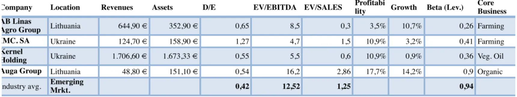
Finding an appropriate peer for the Maragro Group is not an easy task, as the geographical location, the core businesses and the capital structure, as well as the size, shall be taken into consideration. It shall be noted that while the D/E of the firms listed in table (5) is expressed in market terms, for Maragro Group we have to consider a leverage at book value, as the latter is a private company.
In the same table Profitability of the peer group is defined as the EBITDA/Sales margin, whereas the voice growth refers to the 5-years historical growth rate of revenues. The term industry average refers to the market-weighted averages of farming companies operating in the emerging markets.
Company Location Revenues Assets D/E EV/EBITDA EV/SALES Profitability Growth Beta (Lev.) Core Business AB Linas
Agro Group Lithuania 644,90 € 352,90 € 0,65 8,5 0,3 3,5% 10,7% 0,26 Farming IMC. SA Ukraine 124,70 € 158,90 € 1,27 4,7 1,5 10,9% 3,2% 0,41 Farming
Kernel
Holding Ukraine 1.706,60 € 1.673,33 € 0,55 5,5 0,6 10,9% 0,9% 0,36 Veg. Oil Auga Group Lithuania 48,80 € 151,10 € 0,54 16,2 2,86 17,7% 14,2% 0,9 Organic
Industry avg. Emerging Mrkt. 0,42 12,52 1,25 0,94
4.3 Risk-free rate
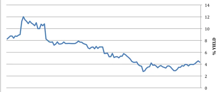
For valuation purposes, it is required to calculate the risk-free rate an investor would receive for investing in a risk-free asset. As for the latter I have used the yield of the 10y Romanian Government Bond, as buying shares of the company is located in that geographical setting and is, more importantly, operating in Romanian Leu. I have chosen a 10-year bond and not a shorter one, as the acquisition of a private company is a long-term investment and is not subject to short-term speculation. As of 31/12/2017, the yield on a 10 y Romanian Government Bond is 4,339%.
Fig. 7 10y. Yield on Rom. Government Bond
0 2 4 6 8 10 12 14 % Y IELD
5 Valuation
5.1 Valuation criteria
The valuation will be performed using the APV methodology. This because a valuation based on multiples is difficult to assess, given the different nature of listed enterprises. In this sense, it is possible to identify similarities with the IMC.SA for what concerns the conventional farming operations. Nevertheless, Maragro Group has a definitely more competitive setup thanks to the high margin processing activity performed by Agrimeies and the production of also organic products. For this reason, we can state that part of the business is similar to the activities of AUGA Group, which nevertheless can also rely on its own brand and is operating in the B2C segment.
Given the above-mentioned characteristics, a discounted cash flow method seems to be more appropriate in evaluating the business, even if we can derive as an initial indication a price range set somewhere in between said peer companies. In deciding whether to choose the classic WACC method or the APV method, I relied on recent literature, which is defining the latter as superior given the decreased number of restrictive assumptions required and thus its
lower risk to incur in massive errors (Luehrman, 1997). Moreover, it shall be noted that
Maragro Group is subject to a change in capital structure in the upcoming years, a fact that reinforces the necessity to apply the APV approach.
I have defined the explicit period as the timeframe 2018-2020. This because, even if the company will reach its operational steady state in 2019, the target capital structure composition will be approached by the end of 2020 with a target D/E of about 0,85.
5.2 Defining the explicit period: Forecast of Revenue Streams
The first step to be done in performing a discounted cash flow valuation is to forecast the revenue streams for the explicit period that has been chosen.
In our case, I have identified five different sources that compose the revenue of the Group i.e. conventional farming activity & related subsidies, organic farming activity & related subsidies, oil mill activity (Agrimeies), service and, finally, trading activity.
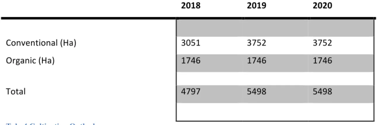
2018 2019 2020 Conventional (Ha) 3051 3752 3752 Organic (Ha) 1746 1746 1746 Total 4797 5498 5498
Tab. 4 Cultivation Outlook
Revenue from the farming activities is influenced by three main factors i.e the amount of hectares cultivated, the yield associated with those hectares and the price of agricultural commodities produced. The most certain data we have at our disposal is the one regarding the amount of land on which the Group can rely for its farming activity and which can be seen in table (6).
Starting from the campaign 2018-2019 (which will be reported in FY 2019), the Group can rely on additional 701 Ha, added to the total platfond of arable land through the rental formula. The cost of this operation is set at 980.650 RON or 1.399 RON/Ha.
As for the harvest of 2018, table (7) shows the Groups’ farming activity. Yield per Ha has been forecasted by the management team based on prior experience and technical data available. Said data can be confronted with the yields of the previous campaign in Annex(II).
Crop Ha Yield t/Ha Revenue Maragro % Price per ton Tons
Sunflower 835 2,5 2.688.700 RON 24,0% 1.288 RON 2088
Wheat 554 5,3 1.632.527 RON 16,7% 556 RON 2936
Seeds 112 4,1 656.370 RON 5,8% 1.430 RON 459
Soybean 769 2,7 2.674.274 RON 23,9% 1.288 RON 2076
Lolium for seeds 720 1,05 3.024.000 RON 27,0% 4.000 RON 756
Rapeseed 61 3 292.800 RON 2,6% 1.600 RON 183
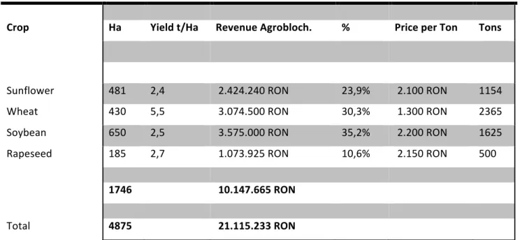
Crop Ha Yield t/Ha Revenue Agrobloch. % Price per Ton Tons
Sunflower 481 2,4 2.424.240 RON 23,9% 2.100 RON 1154
Wheat 430 5,5 3.074.500 RON 30,3% 1.300 RON 2365
Soybean 650 2,5 3.575.000 RON 35,2% 2.200 RON 1625
Rapeseed 185 2,7 1.073.925 RON 10,6% 2.150 RON 500
1746 10.147.665 RON
Total 4875 21.115.233 RON
Tab. 5 Forecast Production Farming
As to predict the revenues of this segment for the following years of the explicit period it shall be noted that a large part of the production is destinated to be transformed by the oil mill facility. Agrimeies in 2018 is expected to transform around 2000 tons of Sunflower, 4400 ton of Soybean and 2000 tons of Rapeseed. It is clear that the majority of inputs needed should be produced at Maragro, as to decrease transportation costs and to benefit from synergies between the companies of the Group. With the introduction of additional 701 Ha in 2019, around 50% of the surface is expected to be dedicated to oilseed production, around 20% to the production of seeds and the remaining 30% to cereals and forage crops.
The most challenging aspect in predicting revenue growth is the one related to the price of the final product. Being Maragro Group a price taker, predictions in this sense have to be made by looking outside of the company and is the result of three different domains. For commodities traded on the exchanges and for which data regarding future contracts until 2021 are available (Soybeans, Wheat) price has been forecasted relying on the predictions of futures. For those for which such information is not available, I have taken data from the agricultural commodities price index (real terms) forecast of governmental sources
Finally, as business is conducted in RON said data is adjusted for the expected fluctuations in exchange rate between the RON and the USD as the above-mentioned futures are quoted in USD on the CBOT while the ACPI is expressed in real 2010 USD. The forecasts for said exchange rates can be seen in tab.(11).
Fig. 8
Finally, yield increase per Ha estimations have been derived from the research article “Yield Trends Are Insufficient to Double Global Crop Production by 2050” (Ray et al., 2013). Said article analyzes the trend in yield gain per country of the four major crops i.e. Maize, Wheat, Soybean and Rice. Unfortunately, as it is not possible to find predictions for the other crops harvested by the Group constant yields have been assumed. This might seem like a limitation assumption, nevertheless, it shall be noted that the effect on the valuation given by said yield increase is of minor impact. Said Yield , as well as future price estimations, can be observed in Annex (II), where it is possible to verify how the farming revenue forecasts for the explicit period have been done.
Directly related to the farming segment, subsidies from government entities are a consequence of the total amount of hectares cultivated, the ecological impact of said cultivations (therefore subsidies for organic farming are higher) and price interventions on strategic commodities.
Commodities Price
In[lation Market Analysis Future ContractsSubsidies 2018 2019 2020
Agroblochberger 3.782.350 RON 3.895.821 RON 3.993.216 RON
Maragro Srl 2.591.255 RON 3.604.475 RON 3.694.587 RON
Inflation 3% 2,50%
Total 6.373.605 RON 7.500.295 RON 7.687.803 RON
Tab. 6 Forecast Subsidies
It shall be noted that for the 3129 Ha of conventional cultivation in 2018, Maragro is only receiving subsidies for 2000 Ha. This is due to agreements made with the owners of the rented properties while the additional subsidies for the Ha expected for 2019 should be entirely perceived by the Group. Table (7) depicts in detail how subsidies have been attributed for the FY 2018. As previously mentioned the amount received is dependent on the hectares cultivated (i.e. 2000 for Maragro Srl and 1746 for Agrimeies Srl), the type of cultivation (organic/conventional) and particular crops which are subject to price regulations (in our case Soybeans).
CAP Contribution 2018 Hectars
Agroblochberger Srl (Organic)
Subsidies PAC 1746 1.400.000 RON
Subsidies for SOYBEANS 650 792.350 RON
Subsedies for bio production 1746 1.400.000 RON
Subsidies for diesel fuel 1746 190.000 RON
3.782.350 RON
Maragro Srl (Conventional)
Subsidies PAC 2000 1.635.760 RON
Subsidies for diesel fuel 2000 ha 2000 218.000 RON
Subsidies for SOYBEANS 605 737.495 RON
2.591.255 RON
For what concerns the trend of Agrimeies, a similar strategy than the one chosen for the forecast of the farming activity has been applied with the exceptions of yield increase, as this does not apply to the oil mill facility which has already reached maximum capacity.
Last but not least, service and trading revenues have been forecasted as to remain constant in proportion to total revenues, respectively 10% and 5% of total revenues. Detailed information regarding the whole revenue forecast can be found in Annex (II).
5.3 Defining the explicit period: Forecast of Operating Costs
In forecasting the operating costs for the following year a distinction has to be made between fixed costs and variable ones i.e. those directly related to the level of output of the company. The latter are listed in detail in Annex (II), while the first can be consulted in table (8).
2017 2018 2019 2020
Fixed Costs 14.600.104 RON 13.074.887 RON 13.687.469 RON 13.904.215 RON
Rent 4.037.012 RON 4.037.012 RON 5.017.662 RON 5.017.662 RON
Personnel 3.413.178 RON 3.597.490 RON 3.705.414 RON 3.798.050 RON Expense / Agr.
Machines 808.326 RON 851.976 RON 877.535 RON 899.473 RON
Cars Expense 148.695 RON 156.725 RON 161.426 RON 165.462 RON
Third Party 4.059.085 RON 1.583.000 RON 1.630.490 RON 1.671.252 RON
Security 260.000 RON 274.040 RON 282.261 RON 289.318 RON
Overhead Costs 1.312.519 RON 1.383.395 RON 1.424.897 RON 1.460.519 RON
Fees 166.427 RON 796.000 RON 180.676 RON 185.193 RON
Costs / oil
production 375.000 RON 395.250 RON 407.108 RON 417.285 RON
Tab. 8 Fixed Costs Frc.
The forecast in table (8) has been made in concordance with the management team. The cost deriving from the rent can be seen to increase from 2019 onwards, as the additional 701Ha have been added at a total yearly cost of 980.650 RON. It shall be noted that, in opposition to the other costs I defined as fixed, this account is not revalued by the inflation rate, as rental contracts in agriculture are defined on a long-term basis. Third party expenses are estimated
its own resources regarding the work to be done. The increase in Fees for 2018 is of exceptional matter, as it reflects the costs that the company is going to incur for the conversion of conventional agricultural land to an organic one. For this reason the account will return to its previous levels from 2019 onwards. It shall be noted that costs related to oil
production include energy costs and those resulting from the purchase of spare parts.
Costs directly related to the output have been provided by the management team for 2018. Concerning the subsequent years of the explicit period, those have been revalued, both, at the forecasted inflation rate and in consideration of the additional hectares mentioned previously. Raw material used by Agrimeies is forecasted in line with the price estimations used to determine revenue from the farming segment, while remaining operating costs are revalued at inflation rate.
Transportation costs have been calculated based on the change in strategy suggested by the management team for the upcoming years. As opposed to the past, Maragro Group will only pay for 10% of the transportation costs, whilst the other 90% will be paid by the customer. This shall decrease double-invoicing of those costs and represent in this way a leaner solution. Over the past two years the expense resulting from paying 100% of those costs resulted in transportation expenses amounting to 2,5% of total sales; thus for the upcoming years I shall consider 0,25% of total sales in order to determine said cost. Detailed data regarding cost construction can be seen in Annex II. As for what concerns the inflation rates used, they can be consulted in table (9)
2018 2019 2020
5,4% 3% 2,5%
5.4 Defining the explicit period: Forecast of Financial Impact
Interest expense for the upcoming years is estimated based on current loans and principal repayment requirements. It shall be noted that the Group has a large need for revolving credit lines given the seasonal nature of incoming cash flows. In this sense, we identify revolving lines of credit for input expenses and anticipation of subsidies. Forecasted interest expenses for the explicit period are shown in table (10), whereas debt composition and future outlook are exhibited in Annex(III).
Key measures of fin. Stability 2017 2018 2019 2020 D/E 7,04 5,26 3,43 2,34 D/E (Adj.) 1,79 1,44 1,12 0,86 Interest Coverage 4,07 4,35 7,94 9,21 Kd 3,27% 3,22% 2,40% 2,40%
Interest 3.052.681 RON 3.284.852 RON 2.252.439 RON 2.084.739 RON
TOTAL DEBT 124.096.922 RON 111.253.231 RON 104.246.314 RON 97.590.190 RON TOTAL EQUITY 17.622.640 RON 21.152.873 RON 30.361.090 RON 41.754.245 RON
Tab. 10 Keyfigures Fin. Stability
Exchange rate plays a major role in the first years of the explicit period. To estimate the change I rely on the concept of purchasing power parity by comparing the estimates for the EUR/RON and the EUR/USD exchange rate as to predict the USD/RON rate. The latter is needed as to calculate price differences between the years of the explicit period, as data on this regard is expressed in USD. The estimates are shown in table (11).
31/12/17 31/12/18 30/04/19
Echange Rate Frc
EUR/USD 1,2006 1,2377 1,2604
The decreasing trend in EUR/RON exchange rate fluctuations in line with the assumptions made in the industry analysis, for which, given the intention of the Romanian government to adopt the European currency, we can expect a decrease in volatility of said rate for the upcoming years. As data extracted from Reuters is only available as of the 30/04/2019, I will take the last forecasts as to estimate profit (losses) due to exchange rate differences for the FY 2019 and 2020.
5.5 Cost of Capital
One major aspect that distinguishes the APV approach from the classical WACC approach is how the cash flows are discounted. By using the APV model I initially discount the future free cash flows to the firm at the unlevered cost of equity. Cost of equity is given by the following formula:
!" = !" + !" − !" × !
Eq. 19 Where,!
= unlevered beta rf = risk-free rate rm-rf = equity premiumIn our case, in deciding the risk-free rate, I considered the 10 years old government bond of Romania, as the company is located in that geographical setting and is, more importantly, adopting the Romanian currency.
The equity risk premium (rm-rf) is derived from data made available through Prof. Damodaran and accounts for the Romanian market to 7,62%.
Last but not least, the beta of the company has been derived by looking at similar enterprises that are listed on the market. By analyzing the core business of the companies I have chosen to derive the beta by taking into consideration the farming revenue and the one derived from product transformation, thus not considering sources such as subsidies, trading and service. I have selected a company for each subsegment (organic or conventional) and applied the betas at a weight reflecting the impact of said subsegment to total sales resulting from those activities. Table (12) provides the scheme used for said beta calculation.
Tab. 12 Calculation of Beta
It shall be noted that, as the unlevered beta is needed for the application of the APV model, we need to unlever our result. This is done by applying the formula shown in eq. (20).
!"#$
1 + 1 − ! ∗
!
!
Eq. 20
As a result of the formula we get an unlevered beta of 0,265 which corresponds to an
Farming Revenue Organic 10.147.665 RON 25% Conventional 10.967.568 RON 27% 11% 21.115.233 RON Product Transformation Organic 11.224.200 RON 28% Conventional 7.586.000 RON 19% 7% 18.810.200 RON 39.925.433 RON Levered Beta Kernel Holding Conventional Oil 0,36 IMC S.A Conventional Farming 0,41 Auga Group Organic Products 0,9 Maragro Group 66,3%
45
5.6 Unlevered firm value
As a result of the forecasted EBITDA I calculated the following free cash flows to the firm: 2018 2019 2020
Revenues 53.841.838 RON 59.734.224 RON 61.638.494 RON
Farming 21.115.233 RON 24.363.974 RON 25.101.334 RON
Subsidies 6.373.605RON 7.500.295RON 7.674.263RON
Agrimeies 18.810.200RON 20.100.872RON 20.899.585RON
Service 6.075.400RON 6.257.662RON 6.414.104RON
Trading 1.467.400RON 1.511.422RON 1.549.208RON
Operating Costs 39.562.250RON 41.853.721RON 42.443.798RON
EBITDA 14.279.587 RON 17.880.503 RON 19.194.696,37 RON
Depreciation 5.507.318 RON 3.884.073 RON 2.971.091 RON
EBIT 8.772.269 RON 13.996.430 RON 16.223.605 RON
Exchange Loss 553.622RON 296.346RON 149.935RON
Tax 1.403.563RON 2.239.429RON 2.595.777RON
CAPEX 2.907.459RON 3.225.648RON 2.971.091RON
Δ NWC 190.954RON 6.449.705RON 2.485.038RON
FCFF 9.223.989 RON 5.669.376 RON 10.992.855 RON
1 2 3
Discounted FCFF 8.672.670 RON 5.011.911 RON 9.137.190 RON
Interest expense 3.284.851 RON 2.252.438 RON 2.084.739 RON
Net Income 3.530.233 RON 9.208.216 RON 11.393.154 RON
Tab. 13 FCFF Forecast
Depreciation has been calculated based on current fixed assets and in consideration of the capital expenditures, I forecasted for the explicit period. For the latter, in absence of data from the management team, assuming a Capex to Sales relationship of 5,4% appeared to be logic. The rate represents the 3-years average CAPEX to Sales relationship of the peer companies taken into reference for calculating the beta. In order to estimate the additional depreciation expense resulting from those capital investments, I have calculated the average duration of the current fixed assets of the Group, weighted by their initial value and amounting to 22,82 years. It shall be noted that for calculation purposes, capital investments equal depreciation expense in the last year of the explicit period. A detailed scheme summarizing the calculations done can be found in Annex (II).
In order to forecast the changes in NWC for the upcoming years, I have taken into consideration the Working Capital needs to total value of production over the past three years.
It shall be noted that the working capital needs are mostly resulting from the farming and oil mill segment. For this reason, I have not considered trading revenues when calculating working capital needs.
The terminal value of 200.893.170 RON is the result of considering the last year of the explicit period as a perpetuity adjusted according to equation (15) by the expected growth rate. For the latter, I have chosen the expected long-term GDP growth of the European Union i.e. 1,73% as shown in fig. (6).
In conclusion, I estimate the unlevered value of the firm to be 223.714.942 RON.
Explicit Period 22.821.772 RON Terminal Value 200.893.170 RON Unlevered Firm Price 223.714.942 RON Tab. 14
5.7 Effects of financing choices
After having calculated the value of the firm as it was entirely financed through equity, it is time to add the effects of the financing choices, starting with the value of the tax shield. Eq. (21) shows an adjusted version of the classical formula used to calculate the terminal value of the tax shields and assumes a constant D/E ratio as opposed to a constant level of debt. Tax shield calculations can be seen in tab. (15).
(!×!×!")×(1 + !)
(!" − !)
Eq. 21where,
D = Outstanding financial debt FY2020 T = Tax rate