Equity valuation using accounting numbers in high and low intangible-intensive industries

(1)

Equity Valuation Using Accounting Numbers in High and Low

Intangible-Intensive Industries

Rita Albuquerque Silva (152110043)

Advisor: Ricardo Ferreira Reis

Dissertation submitted in partial fulfilment of requirements for the degree of MSc in Business Administration, at Católica Lisbon School of Business and Economics, 17th September 2012

(2)

Abstract

Recent scandals in companies such as Enron, WorldCom or Tesco have become practical solid examples of accounting manipulation and have been disrupting the accountancy field. As a consequence, there has been a regular reinforcement regarding the practical use of accounting numbers. Equity valuation using accounting numbers plays a vital responsibility in both finance and accounting areas, grounding on the use and comparison of valuation models’ performance.

This dissertation aims to explore the association between high and low intangible-intensive industries as well as the performance of accounting-based valuation models. After assessing not only stock- but also flow-based models across the two industries, results reveal a superior performance of the former models for low intangible-intensive industries while flow-based models disclose superior stock price predictions for high intangible-intensive industries. In complement, an analysis of the valuation techniques applied in analysts’ reports demonstrates that marked multiples are usually the preferred methodology for equity research analysts to value companies.

Key Words: Intangible assets, high/low intangible-intensive industries, stock-based

(3)

I Contents

Abstract ... 2

II List of Figures ... 5

III List of Tables ... 5

IV Notations and Abbreviations ... 6

Introduction ... 8

1.1 Background and Motivation to Research ... 8

1.2 The Research Problem ... 8

1.3 Outline ... 9

Review of Literature in Equity Valuation ... 10

2.1 Introduction ... 10

2.2 Usefulness of Accounting Income Numbers ... 10

2.3 Accounting-Based Valuation Models ... 11

2.3.1 Business-Valuation Perspectives ... 11

2.3.2 Stock-Based Valuation Models ... 12

2.3.2.1 Selecting Comparable Firms ... 13

2.3.2.3 Selecting Value Drivers ... 15

2.3.3 Flow-Based Valuation Models ... 15

2.3.3.1 Dividend Discount Model (DDM) ... 15

2.3.3.2 Discounted Free Cash Flow Model (DFCFM) ... 16

2.3.3.3 Residual Income Valuation Model (RIVM) ... 17

2.3.3.4 Abnormal Earnings Growth Model (AEGM) ... 19

2.5 Discussion of Valuation Model Performance ... 20

2.6 Concluding Remarks ... 21

Large Sample Analysis ... 22

3.1 Research Question and Literature ... 23

3.2 Data and Sample Selection ... 23

3.3 Research Design ... 25

3.3.1 Stock-Based Valuation ... 26

(4)

3.3.1.2 Comparable Firms Selection ... 26

3.3.1.3 Benchmark Multiples ... 26

3.3.2 Flow-Based Valuation ... 26

3.3.2.1 Cost of Capital (k) ... 27

3.3.2.2 Earnings per Share (EPS) ... 27

3.3.2.3 Dividend Payout Rate ... 27

3.3.2.4 Growth-Rate ... 27

3.4 Empirical Results ... 28

3.4.1 Descriptive Statistics ... 28

3.4.2 Analysis of Valuation Errors ... 29

3.4.2.1 Intra-Sample Analysis of Valuation Errors ... 30

3.4.2.2 Cross-Sample Analysis of Valuation Errors ... 33

3.4.2.3 Difference in Valuation Errors Between Valuation Models ... 34

3.4.2.4 Explanatory Power of Accounting-Based Valuation Models ... 36

3.5 Concluding Remarks on Empirical Results ... 37

Small Sample Analysis ... 39

4.1 Hypothesis and Main Literature ... 39

4.2 Data and Sample selection ... 40

4.3 Research Design ... 41

4.3.1 Primary valuation models ... 42

4.3.2Analysts’ recommendations ... 44

4.4.3 Forecast horizon in analysts’ reports ... 46

4.4.4 Supplement analysis on key firms’ characteristics ... 47

4.4.4.1 Market size ... 47 4.4.4.2 Volatility – beta (ρ) ... 49 4.4.4.3 Analyst Coverage ... 50 4.5 Concluding remarks ... 52 Conclusion ... 53 V Appendix ... 59

(5)

II List of Figures

Figure 1 - Intangible to tangible ratio growth in UK

III List of Tables

Table 1 – Sample selection (untrimmed data) Table 2 – Untrimmed sample descriptive statistics Table 3 – Trimmed sample descriptive statistics

Table 4 – Descriptive statistics of valuation errors (trimmed data) Table 5 – Intra-sample valuation accuracy and bias

Table 6 – Cross-sample analysis of valuation errors Table 7 – Models’ valuation performance

Table 8 – Explanatory power of valuation models

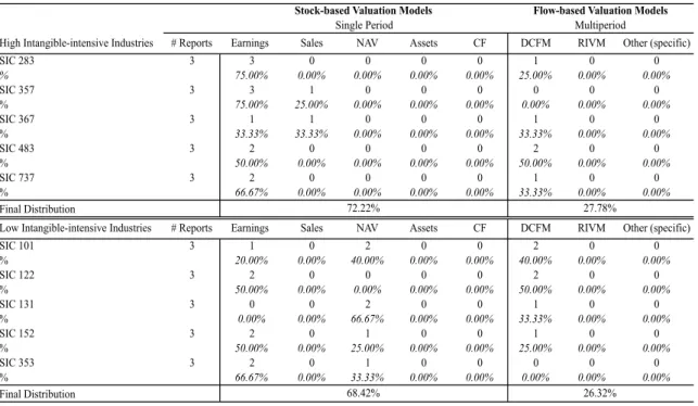
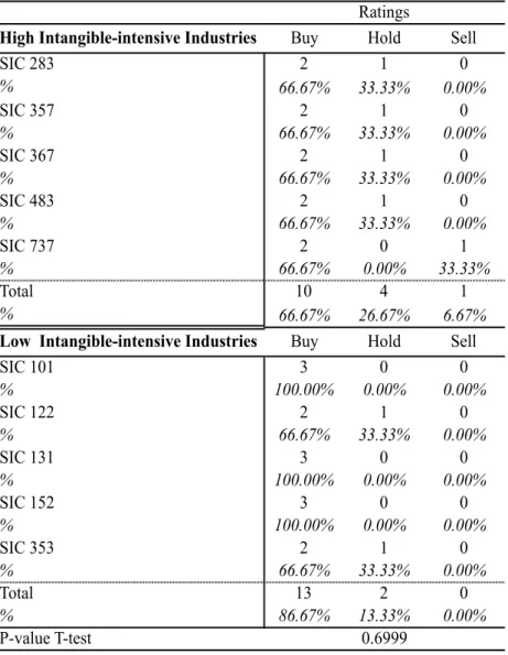
Table 9 – Firms belonging to high and low intangible-intensive industries Table 10 – Valuation models employed by analysts in the two samples Table 11 – Analysts’ ratings for high and low intangible-intensive industries Table 12 – Forecast horizons for small sample firms

Table 13 – Market size of the firms in the small sample analysis Table 14 – Volatility (beta) of the small sample firms

Table 15 – Analyst coverage for the two sample firms in the small sample data

(6)

IV Notations and Abbreviations

AEGM DCF DDM DFCFM e.g. E&P EPS EV EVA GAAP I/B/E/S IAS IFRS IPO LBO NOPAT M&M Max MDFY1/2 Min NAV P/E P1 P99 PLC Q1 Q3 R&D RIVM SD SIC SEO

Abnormal earnings growth valuation model Discounted cash flow

Dividend discount model

Discounted free cash flow model Example given

Energy and petroleum Earnings per share Enterprise value Economic value added

Generally accepted accounting principles Institutional brokers' estimation system International accounting standards

International financial reporting standards Initial public offering

Leverage buyout

Net operating profit after tax Modigliani and Miller Maximum value

1 and 2 year-ahead forecast earnings Minimum value

Net asset value Price earnings ratio 1st percentile 99th percentile

Public limited company 1st quartile

3rd_quartile

Research and development

Residual Income Valuation Model Standard Deviation

Standard Industry Classification Seasoned equity offerings

(7)

SSA SSB TV UK Sub-sample A Sub-sample B Terminal value United Kingdom

(8)

Chapter 1 Introduction

1.1 Background and Motivation to Research

Presently, terms as ‘the new economy’ and ‘intangible assets’ are powerfully connected. Intangible assets are becoming extremely important to the continued growth and development of the modern economy and well being of citizens.

International Accounting Standards (IAS) defines an asset as: a resource controlled by a firm as a result of past events from which future economic benefits are expected to flow to the entity in the future. According to Constantin et al. (1994) this asset category can still be separated in tangible or intangible, included in the balance sheet or not, and internally or externally created (Srivastava et al., 1998).

Although no consensus has yet been reached for the definition of an intangible asset, it can be expressed as an identifiable, non-monetary asset, lacking physical substance (Stolowy and Cazavan, 2001). For Wyatt (2005) and Lev (2004), examples of intangible assets include patents, trademarks, brands, licenses, technology, employee training, know-how, skilled workforces, and customer loyalty, amongst others.

The continuing transition to a more knowledge-based and technology intensive economy is causing intangible assets to be essential to preserve firm’s competitive position and to their value creation process (Holland, 2001; Lev, 2001; Sullivan and Sullivan, 2000; and Sveiby, 1997).

1.2 The Research Problem

If, as intelligible by the former section, intangibles are becoming so indispensable, they need to be correctly treated and formalised (Vance, 2001). The opposite will create unbiased and unfair results of firms’ performance (Cañibano et al. 1999).

Once the source of economic value is also the wealth creation of intangible assets, firms are increasing the need to make investments associated with this assets’ class (Cañibano et al. 1999). However, the limited accounting criteria related to the recognition of assets and their valuation leads to uncovered investments in the balance sheet. Therefore, the

(9)

issue of financial statements not being able to reflect complete information of companies’ financial position, providing reliable but not relevant value estimations, is being subject to debate (Cañibano et al., 2000).

1.3 Outline

Based on the topic that intangible assets are difficult to be perfectly measured, even though reflecting superior growth opportunities and earnings for companies, this study focus on the examination of equity valuation models’ performance across high and low intangible-intensive industries. The main purpose is to compare models’ results and evaluate whether the primary differences between the two industry groups considerably influence the performance of valuation techniques.

A large sample analysis will determine the valuation of both high and low intangible-intensive industries using accounting-based valuation models to, first, identify similarities and differences across industries and, second, to conclude whether (or not) there is a better valuation model for each group, reflecting lower valuation errors and, consequently, superior estimates. Next, a small sample analysis will assess the valuation approaches used by specialists to value both industries.

The study is structure as follows: the next chapter presents the main literature concerning equity valuation using accounting-based valuation models. Chapter 3 identifies and examines the results of the large sample analysis. Chapter 4 encompasses a small sample of analysts’ reports, evaluating the chosen valuation techniques, forecast horizons and recommendations. In addition, it connects specific firms’ characteristics with both industry samples. Finally, chapter 5 concludes the study with a summary of the major results and comments on the fields for further research.

(10)

Chapter 2 Review of Literature in Equity Valuation

2.1 Introduction

Equity valuation can shortly be defined as the task of forecasting the present value of the stream of expected payoffs to shareholders (Lee, 1999). Mostly at any level it can be implied that every business decision comprises valuation. On one hand, within the firm, capital budgeting and strategic planning involve the deliberation of the impact a project can have in firm value and how can value be subject to a set of actions, respectively. On the other hand, outside the firm, analysts resort to valuation so as to reinforce their ratings decisions while delivering forecast of value of target companies and the synergies that can be produced (Palepu et al., 1999).

In practice, equity valuation encompasses diverse valuation models. Nowadays, according to Damodaran (2002) and (2007) the main valuation models range from absolute valuation, relative valuation, returns based valuation and, finally to contingent claim valuation.

The following section will start with a brief reflection regarding the informational content of financial statements. The main objective is to introduce a more complex discussion of the different accounting-based valuation models and present the body of literature served as for the theoretical grounding of this study.

2.2 Usefulness of Accounting Income Numbers

According to Lee (1999), valuation is as much as an ‘art’ as it is a ‘science’. It comprises looking into an uncertain future, and making what can be referred as an ‘educated guess’. Complete objectivity is hard to achieve. Lee enforces, as a key concept to valuation, the helpfulness of information in order to estimate value. Therefore, reported accounting numbers in addition to other material, provide a comprehensive basis of information on a firm. In published financial statements, earnings are believed to be the primary information item available. Many equity valuation models share the same explanatory variable - expected earnings. Accordingly, the variable provides an adequate measure of

(11)

value (Burgstahler and Dichev, 1997).

The content of income numbers can be analysed by testing how stock prices reproduce the flow of information. Ball and Brown (1968) refer that, when reported income distinguishes itself from expected income, information present in annual income figures seems to be especially useful to investors and highly linked to stock price. They limit the idea of earnings as a useful measure due to the fact that annual reports are not timely medium and, instead, their content is captured by more prompt media1_.

2.3 Accounting-Based Valuation Models

The wide number of accounting-based valuation models can essentially be distinguished into two main approaches – the stock-based and flow-based. While the latter depends on a diverse amount of estimated inputs, the former does not.

The next section introduces the central perspectives concerning business valuation and summaries five accounting-based valuation models, their pros and cons, relation to other models and implementation issues.

2.3.1 Business-Valuation Perspectives

Valuation models can be structured in two ways. The first – equity perspective2_{- values} straight the equity of the firm; once this is normally the variable analysts are interested in estimating. It distinguishes the capital provided by shareholders and debt holders. The second – entity perspective3 - values firms´ assets, which corresponds to valuing the claims equity and valuing the net debt and to remove the value of net debt. Theoretically, both approaches should generate the same values (Palepu et. al, 1999).

Under the equity perspective, the reporting entity is supposed to have no substance of its own separate from that of its proprietors or owners. Consequently, financial reporting from the equity perspective comprises reporting on the assets of the owners (Financial Accounting Standards Board, 2008).

1_{Inclusion of interim reports}

2_{Referred also as proprietary perspective} 3_{Referred also as enterprise perspective}

(12)

The accounting equation for this perspective equals (Financial Accounting Standards Board, 2008):

!""#$" − !"#$"%"&"'( = !"#!"# ⟺ !"# !""#$" = !"#$%& (1) For the entity perspective, the accounting equation is the following (Financial Accounting Standards Board, 2008):

!""#$" = !"#$%&'" !"#$%$&' + !"#$% !"#$%$!" (2) or

!""#$" = !"#$%&'" !"#$%& + !"#$% !"#$%& (3) or

!""#$" = !"#$%& (4) While the equity perspective makes a distinction between the different sources of capital, the entity perspective ignores them totally. The latter does not suffer so much from financing differences and allows for a better value estimate, since managers’ financing decisions do not interfere. When differences in accounting affect entity valuations or valuations are less meaningful, this approach is clearly preferable. Furthermore, the equity perspective tends to dominate the entity perspective due to the weight it places on equity investment and stock markets. The downside of equity-based value estimates is the link with firm-specific financing decisions, which reduces the usefulness of a comparison across firms.

2.3.2 Stock-Based Valuation Models

Stock-based valuation models, specifically, multiples-based models, contrast with flow-based models once the first does not comprise a multi-year forecasts of a series of parameters such as earnings, growth, discount rates and others (Palepu et. al, 1999). Market-multiples´ models investigate the proximity to stock prices of valuations generated by multiplying a value driver by the corresponding multiple, with the multiple being obtained from the ratio of stock price to the value driver for a group of comparable firms (Liu et al., 2002). Multiples is an well-liked method in equity valuation (Carter and

(13)

Van Auken, 1990) due to their simplicity in comprehension and easiness in communication (Liu et al., 2002). Additionally, it is employed not only by analysts but also by investment bankers, IPOs, LBOs, SEOs and other merger and acquisition transactions (Bhojraj and Lee, 2002).

Under the stock-based valuation approach, analysts trust on the market to start the task of forecasting both short- and long-term profitability and growth as well as their repercussions in the “comparable” firms’ values. Since there is a reflection of the market, the value should be considered relative and intrinsic (Palepu et al. 2000).

In summary, valuation using multiples involve the following steps: First, identify comparable companies, which comprise analogous operations when compared to those of the target firm whose value is being calculated and identify and select value drivers (e.g., earnings, cash flows, sales,book assets, book equity). Second, calculate the benchmark multiple from comparable firms and then, third, apply this benchmark multiple to the performance or value measure of the firm being analysed (Palepu et al. 2000).

The main assumptions of this model are: (1) future cash flows of comparable firms are similar to those of the target, (2) the risk profiles of comparable firms are similar to the target and (3) the value driver is proportional to value.

The general method for multiple-valuation can be written as:

!_! = !"_! × !"#$ℎ!"#$ !"#$%&#' (!_!) (5) Where !_!is the value estimated for firmi, !"_!symbolizes the value driver (where!"_! > 0) and !! reflects the set of comparable firms for firm i.

In conformity with section 2.2.1, there are two fundamental perspectives that can be applied to the different models. The multiple-based valuation model is not an exception, either equity or entity values can be estimated. For the first case, VD! is an equity value driver (e.g. Net Income) while for the second case, VD_! represents an entity value driver (e.g. NOPAT).

2.3.2.1 Selecting Comparable Firms

(14)

the identification of ‘comparable’ firms is often quite difficult due to its nature as a valuation heuristic. The best case scenario possible when applying price multiples is the one involving firms with similar operating and financial businesses, resulting in companies within the same industry being the most desirable candidates. Nevertheless, even industries that are strictly defined present difficulties when finding multiples for similar companies (Palepu et al. 2000). As Liu et al. (2002) argue, firms sharing the same industry reveal differences regarding strategies, profitability and goals, originating comparability issues.

Two solutions can be implemented in order to solve some of these issues. First, an average across all firms in the industry can be applied to ‘cancel out’ diverse sources of noncomparability. The second solution is to focus only on the most similar companies, which share the same industry (Palepu et al., 2000; Boatsman and Baskin, 1981).

An important study associated with comparables is carried by Alford (1992), who concludes that valuations using comparables chosen by their 3-digit SIC code is a good proxy for industry specific characteristics.

2.3.2.2 Calculating the Benchmark Multiple

Complementing the implementation issue of comparables is the issue that preferable applied drivers in multiples are more volatile than equity prices, resulting in comparable firm multiples being quite dispersed (Fernández, 2002). Thus, a statistic estimator able to summarise a benchmark multiple is compulsory. The most popular are presented next:

-‐ Mean arithmetic average =!_! ! _!"#!"

!!! (6) -‐ Median = midpoint of observed values´ frequency distribution (7)

-‐ Weighted average = !!"#_!"# !!! ! !!! × _!"#!" = !" ! !!! !"# ! !!! (8) -‐ Harmonic mean = ! ! ! !"# !" ! !!! (9)

Where !" _!denotes the value driver and !_! the observed price for the !!!_{comparator firm.} Baker and Ruback (1999) defend that the harmonic mean (9) use delivers superior valuation performance compared to the other three outlined estimators (6,7 and 8). In fact, the authors point out that multiples resulting from the simple mean tend to overvalue. The

(15)

mean-based estimation will always return a higher number than the harmonic mean value, which yields less upward-biased estimates.

2.3.2.3 Selecting Value Drivers

Value drivers are an important input for multiple valuations and should reflect a proper proxy for firm’s performance. Forecasted earnings are the most common used value driver due to their high informational content. Nevertheless, their selection depends on the company and the industry they are assigned to. Multiples using forecasted earnings as value driver have a better performance, with valuation results being improved with the forecast horizon (Liu et al., 2002 and Fernández, 2002).

Liu et al. (2002) in their study find that multiples using estimated earnings as value drivers outperform multiples using reported earnings across different GAAP jurisdictions. Additionally, Liu et al. (2007) reinforces the popularity of P/E-multiples by showing that valuations based on earnings multiples are preferable for the majority of companies due to its stronger accuracy compared to value estimates from cash flow multiples.

2.3.3 Flow-Based Valuation Models

The following flow-based valuation techniques presented ground on the notion that the market value of a share is the discounted value of the expected future payoffs generated by the share. Although payoffs can diverge, under a set of conditions, models produce theoretically correspondent measures of intrinsic value.

2.3.3.1 Dividend Discount Model (DDM)

Valuations models derive, more or less obviously, from the DDM attributed to Williams (1938), making it a reference for almost all valuation techniques (Barker, 2001).

Dividends are equivalent to the cash flows distributed to shareholders and reported in the cash flow statement (Penman, 2007). The main supposition lies on the fact that the market value of equity capital is defined as the sum of discounted future net cash flows. DDM (equity version) estimates the value of a stock by computing the present value of the expected future cash dividends (Ross et al., 2008). Thus:

(16)

The subsequent formula states the dividend discount model:

!_!!"#₌ !"#!

(!!!!)!

!

!!! (10)

Where !"#_!denotes the dividends and !_! the equity cost of capital.

The DDM is the simplest model used in equity valuation and it is also the most essential and important flow-based model. DDM preferences from investors have to do with the forecasting task, which is very straightforward and easy, assumed stable dividend policies (Brealey et. al 2005; Penman, 2008). However, the main limitation is the requirement that dividend forecasts to infinity. Copeland et al. (2008), in order to deal with the problem, suggest splitting business value into two periods, during and after the explicit forecasting period. The value beyond the forecast horizon is a terminal value featuring a continuous growth rate.

Other limitation is DDM association with Modigliani and Miller’s (1961) dividend irrelevance proposition. Many researchers do not agree with M&M proposition and state the dividend’s contribution in valuation. Both Walter (1956) and Black and Scholes (1974) concluded that a change in dividend policy affects stock price. Besides, Fisher (1961) explains that dividend and profit have analogous effects on share prices.

2.3.3.2 Discounted Free Cash Flow Model (DFCFM)

The discounted free cash flow model is based on the DDM, with the difference being that it replaces free cash flows for dividends since it assumes free cash flows to be a better demonstration of value added over a short horizon.

Free cash flows equal the cash available to the firm's providers of capital after all required investments. Algebraically it can be represented as (Francis, et al. 2000):

FCF_! = Sales_!− OPEXP_!− DEPEXP_! (1 − τ) + DEPEXP_!− ∆WC_!− CAPEXP_! (11) Where Sales_! equals sales revenues for year t; OPEXP_! denotes operating expenses for year t; DEPEXP! expresses depreciation expense for year t; ∆WC! represents the change on working capital in year t and CAPEXP_! is equivalent to capital expenditures in year t. Thus, the final model is expressed as the following (Francis et. al, 2000):

(17)

V_!!"!₌ !"! (!!!"##)!+ !

!!! ECMS! + D!+ PS! (12) Where ECMS_! is equal to the excess cash and marketable securities at time t;D_!is the market value of the debt at time t and PS! illustrates the market value of preferred stock at time t.

With:

WACC = w_! 1 − τ r_!+ w_!"r_!"+ w_!r_! (13) Where WACC expresses the weighted average cost of capital; r_! equals the cost of debt; r!" denotes the cost of preferred stock; w! is the proportion of debt in target capital structure; w_!" is equivalent to the proportion of preferred stock in target capital structure; w_!is the proportion of equity in target capital structure and τ the corporate tax rate. The main model’s limitation is the fact that the free cash flow does not really add value in operations. It confuses investments with the payoffs from investments since it is somewhat an investment or a liquidation concept (Penman, 2007).

Another practical problem is the fact that free cash flows, in contrast to earnings, are not exactly what analysts forecast.

2.3.3.3 Residual Income Valuation Model (RIVM)

Residual income, or abnormal earnings, plays a protuberant role in equity valuation, being used as a measure of performance (O’Hanlon, 2002). According to Ohlson (1995), residual earnings are equal to accounting earnings less a cost of capital based on the opening book value of equity (14). This meaning is analogous to the economic value added (EVA) concept and, based on Lee (1996), the development of the RIV model corresponds to the EVA paradigm.

The traditional RIV model approach, based on an equity perspective, rests on the assumptions that company’s value equals the present value of expected future dividends and both earnings and book value forecasts result from a Clean Surplus Relationship (CSR). According to this relationship, (15) earnings equal the change in book value of equity plus dividends net of capital (O’Hanlon, 2009). Thus, the intuition behind the

(18)

derivation of the residual income model is to exactly use book value and forecasted future earnings (premium) to back out dividends using the clean surplus relation (16).4

!"_!! _{= !"} !− !! × !"#!!! (14) !"#_!− !"#_!!!= !"_!− !"#_! (15) !_!! _{= !"#} !+ !!!!!!! ! (!!!!)! ! !!! (16)

When compared to market multiples, the RIVM is able to address some of the model’s implementation issues, essentially due to its easiness in obtaining the computations of equity values, by focusing on observed book values, return on equity and equity cost of capital (Bryan et al, 2001). When comparing the RIVM final values with extra available estimations from the dividend discount and cash flow models, empirical studies conclude that residual-earnings-based value estimates are superior. The reasons stated include (1) the model’s support in book values, explaining a larger proportion of intrinsic value and (2) the use of more precise earnings forecasts (Courteau et al. 2007).

Accounting discretion and accounting conservatism have been explained as two of the main limitations of accounting-based valuation models although they do not seem to have any impact on the reliability of residual earnings estimates (Francis et. al, 2000).

Along the last years, researchers have been studying the usefulness of the RIVM value estimates. By comparing the value estimates of the three different (DD, DFCF and RIV) models, RIVM shows to be the most accurate and the one explaining more variation in stock price (Penman and Sougiannis, 1998; Francis et al., 2000). Besides, researchers also found that earnings approaches do not have a good performance for high numbers of both price-to-earnings and price-to-book. In this case, terminal value calculations are relevant for valuation.

Among several researchers, the RIV model is preferred as a superior technique for valuation within finite horizons (Penman and Sougiannis, 1998 and Francis et al., 2000) However, the RIVM and the DCFM have equal value estimates when complete pro-forma statements are available (Lundholm and O’Keefe, 2001).

(19)

The limitations of the RIV model are highlighted by Ohlson and Juetter-Nauroth (2005), stating the model’s dependency on the clean surplus relationship and its anchorage in book values. First, the application of the RIVM requires a clean surplus relationship on a per share basis. Second, it is not possible to avoid the per share issue, by applying the RIVM on a total dollar value basis. Concluding, Ohlson (2005) claims the RIVM inability to generate per-share value estimates if M&M restrictions are not re-introduced. Consequently, Ohlson and Juettner-Nauroth (2005) created the abnormal earnings growth model (AEGM) through the expansion of RIVM, by relating a firm’s share price to its capitalised next period earnings, its short and long term earnings growth and cost of equity capital.

2.3.3.4 Abnormal Earnings Growth Model (AEGM)

In accordance with the RIV model, the AEG model, also known as Ohlson/Juettner-Nauroth (OJ) model, conceptually grounds on the same mathematical structure as the RIVM. In addition, it starts from the present value of future dividends 5(Penman, 2008; O'Hanlon, 2009). Ohlson (2005), the residual earnings valuation framework developer, forecasts an actual replacement of the RIVM by the AEGM, since the former is aligned with analysts’ focus on earnings. The AEGM model, on the contrary, defines intrinsic value of equity as capitalised, next-period earnings plus the present value of capitalised, forecasted abnormal earnings growth in succeeding periods (12) (Ohlson and Juetter-Nauroth, 2005). Abnormal earnings growth is defined as the difference between periodic earnings change and a normal return on previous-period earnings (13) (Ohlson and Juetter-Nauroth, 2005). !_!! ₌!! !"!!! !! + !!!!!! (!!!!)! ! !!! (17) !! = _!! ! ∆!"!!!− !! (!"!− !"#!) (18)

The AEGM is able to overcome shortcomings of the RIVM since it relies on capitalised, next period earnings. Thus, the model expresses its premium as successive increments in expected earnings adjusted for dividends (O’Hanlon, 2009). It does not demand an anchor on book values and does not rely on the notion of a CSR. Thus, a valuation per-share on a

(20)

total dollar basis is possible and capital transactions’ undesirable effects are disregarded (Ohlson, 2005).

The practitioner’s advantage side is the model’s focus on earnings, the main catalyst for value creation. The idea underlined is that ex-ante capitalized earnings approximate market value more closely than book values (Ohlson, 2005).

2.5 Discussion of Valuation Model Performance

In accordance to Demirakos et al. (2004), the discussion between academics and practitioners , with regard to valuation models, remains. If multi-period valuation models are theoretically superior there is a weak practitioners’ application.

Gleason et al. (2008) enlarged the number of arguments in favour of flow-based valuation models. According to the authors, the application of flow-based valuation models by analysts brings a significantly improved accuracy in the calculation of price targets. This fact enables to highlight the quality deterioration when the calculation is based on valuation heuristics as well as on inaccurate earnings forecasts.

Although the usual academic position, practitioners tend to apply stock-based models. Valuation heuristics are normally applied as a bottom line for firm valuation and combined, if necessary, with more complex models (Barker, 1999).

Courteau et al. (2007) shows that flow-based models performance are superior to multiples, regarding pricing and return-prediction. Nonetheless, they provide empirical evidence of companies’ analysis improvement by combining a multiples valuation with flow-based valuation frameworks.

In contrast, Imam et al. (2008) claims that practitioners have a preference for flow-based valuation models, highlighting the models’ preference role as a key valuation technique in analysts reports, when compared to accrual-based models. However, valuation accuracy is not improved by cash flow-based valuation (Imam et al., 2008). Sougiannis and Yaekura (2001), Fernández (2002), and Imam et al. (2008) highlight the fact that multiples are extensively used when combined with more sophisticated frameworks. Apart from stock- or flow-based, accounting-based valuation models are subject to

(21)

inaccuracies primarily attributed to: accounting measurement errors; quality of earnings forecasts; specifications; and the efficient market hypothesis.

Tasker (1998) states that the effectiveness of accounting rules performance across industries affects accounting-based valuation profoundly. The most evident source of valuation errors and accounting-based valuation models’ performance are endorsed to the inferiority of GAAP earnings. Particularly, losing firms, even though demonstrating high growth and/or high R&D-expenses, they are jeopardized by conservative accounting rules once they reduce book values and reported earnings’ informational content. Sougiannis and Yaekura (2000) suggest that applying longer forecast horizons can overcome current losses and R&D-expenses.

2.6 Concluding Remarks

The previous section comprised the main literature and theoretical foundation of accounting-based equity valuation. Flow-based valuation models seem to show superiority compared to stock-based valuation models, specifically, market multiples. Nevertheless, practitioners frequently decide to use this last model in valuations.

The following section will employ part of the valuation models presented to a sample of high and low-intensive intangible firms. The objective is to conclude if valuation performance across certain accounting-based models is subjective to company’s asset structure.

(22)

Chapter 3 Large Sample Analysis

As outlined in chapter 1, accounting numbers do not always reflect fair value at a specific moment in time. Specifically, companies with a high level of investments, whether in brand names or in R&D and advertising, do not have this amount of value recognised in the balance sheet.

Nowadays, consumers are usually more willing to buy advertised brands due to a superior sense of trust and brand awareness. Thus, companies are currently spending money on the intangibles´ asset class in order to realize future revenue potential (Figure 1).

Figure 1 – Intangible to tangible ratio growth in the UK

When a company builds a plant or purchases equipment, the asset is capitalised on the balance sheet and depreciated over time. Conversely, when a company creates an intangible asset, such as a brand name or patent, the entire outlay must be expensed immediately. For firms with significant intangible assets, such as technology companies and pharmaceuticals, failure to recognize intangible assets can lead to a significant underestimation of a company’s invested capital and, thus, overstate return on invested

1970 1975 1980 1985 1990 1995 2000 1.4 1.2 1.0 0.8 0.6 0.4 0.2 0.0

Source: HMT (2007) Intangible Investment and Britain’s Productivity: Working Paper no 1.

(23)

capital (ROIC) (Koller et al., 2005).

3.1 Research Question and Literature

According to Hall (2001), the valuation effect of intangible assets in firms’ market value is more important than that of tangible assets.

Recent research by Amir and Lev (1996) has achieved a mark in the area of intangibles. They evaluate the roles of accounting and nonfinancial information in the valuation of cellular phone companies. Results reveal that financial information is largely irrelevant in valuing U.S. cellular phone companies once accounting requires the immediate expense of customer acquisition costs.

As mentioned on section 2.3, valuation models should give the same or similar intrinsic value. Nevertheless, some models can indeed outperform others according to different assumptions and input variables. Similarly, industry characteristics matters, in fact, specific models result in superior performances in particular industries.

The large sample analysis section of the study aims to evaluate if the use of disparate valuations models give different results according to different industry groups. By having two distinctive groups, questioning whether (or not) the valuation model applied is different reveals to be a valuable study. In addition, it is pertinent to evaluate the performance of different models for each of the underlying groups, separately. The main hypothesis of the analysis consists on the fact that differences in earnings patterns and industry characteristics influence models’ valuation performance. Thus, a firm’s industry characteristic is able to determine the capacity of a model to capture firm value. The study of models’ performance is based on the accuracy and bias of value estimates.

3.2 Data and Sample Selection

The original data used to perform the large sample analysis is grounded on values from the I/B/E/S and COMPUSTAT databases and includes 11.493 observations of annual firms’ accounting data, share prices and analysts forecasts for U.S. public firms between 2005 and 2010.

(24)

statements as of 31st_{December and I/B/E/S gathers and summarises analysts’ forecasts} from a broad cross-section of equity analysts as of 15th April.

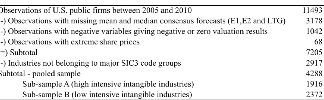
The sampling selection process described in table 1 excludes from the original sample provided observations with missing or negative 1-year, 2-year and long-term I/B/E/S earnings forecasts and negative values of earnings per share as well as extreme (low and high) share prices (2<P<300). The objective is to guarantee that all valuation models result in reasonable results. Afterwards, observations not belonging to major SIC code groups were excluded from the original sample. The criteria assents on the rational that industries with less than 0.75% frequency distribution of observations do not reflect and are not representative of an industry class.

The selection of high vis-à-vis low intangible-intensive industries is based on a study by Collins et al. (1997), which defines firms as intangible intensive when their production function likely include large amounts of unrecorded intangibles.

The grounding literature is, again, based on Collins et al. (1997), where intangible-intensive firms belong to the two-digit SIC codes: 48 (electronic components and accessories), 73 (business services), 87 (engineering, accounting, R&D and management related services); and three-digit SIC codes: 282 (plastics and synthetic materials), 283(drugs), and 357 (computer and office equipment). This study permits to extrapolate the high intangible-intensive industries as fitting to the previously mentioned SIC codes. The two-digit SIC codes (48, 73 and 87) were amplified to include all the three-digit SIC codes, once these provide better performance results (Alford, 1992).The low intangible-intensive industries are the remaining SICs not belonging to the high intangible-intangible-intensive industry sample (Collins et al., 1997).

Furthermore, it is necessary to note that, in this study, intangible intensity does not refer only to the presence of large amounts of recorded intangibles once the research question also tries to capture unrecorded intangibles (Collins et al., 1997).

(25)

Table 1 – Sample selection (untrimmed data)

The selection process generates three final outputs. This selection enables an overall analysis of specific industry characteristic groups by focusing on the comparison of valuation accuracy, valuation bias, and explanatory power both on an aggregate and disaggregated level.

3.3 Research Design

In order to compare accounting-based valuation models and to conclude their performance across high and low intangible-intensive industries, the empirical analysis section comprises three main valuation models; one stock-flow based model represented by the P/E multiple6 and two flow-based valuation models reflected by the RIVM and AEGM.

Valuation model performance is consistent with the methodology applied by Lie and Lie (2002), Liu et al. (2002) and Corteau et al. (2007). The rational is based on the argument that valuation errors reflect reasonable measures of model’s accuracy and bias. Valuation bias is measured by signed valuation errors (19) and represents the model’s tendency to under- or overvalue as a percentage of price at valuation date.

!"#$%& !"#$"%&'( !""#"_! = !"!! !!

!! (19)

Valuation accuracy is measured by absolute valuation errors (20) and represents the percentage of price at valuation date not incorporated by the value estimate.

6_{From now on abbreviated as P/E}

Observations of U.S. public firms between 2005 and 2010 11493 (-) Observations with missing mean and median consensus forecasts (E1,E2 and LTG) 3178 (-) Observations with negative variables giving negative or zero valuation results 1042 (-) Observations with extreme share prices 68

(=) Subtotal 7205

(-) Industries not belonging to major SIC3 code groups 2917

Subtotal - pooled sample 4288

Sub-sample A (high intensive intangible industries) 1916 Sub-sample B (low intensive intangible industries) 2372

Table 2 describes the sample selection process regarding the untrimmed data. The first subtotal is obtained by retaining the non-missing mean and median consensus forecasts for long-term growth (LGT), one- (E1) and two-year-ahead (E2) forecasts. In addition, the negative variables are excluded as well as the missing and extreme share prices available. To determine the pooled sample, industries with less than 0.75% frequency distribution of observations are also excluded. Finally, based on Collins et al. (1997) the selection of high- and low intangible-intensive industries is made.

(26)

!"#$%&'( !"#$"%&'( !!!"! _! = !"!! !!

!! (20)

Where VE! reflects the value estimate and P! the price at valuation date.

3.3.1 Stock-Based Valuation

The details of the P/E multiple, as well as the assumptions and steps required to derive the model, are presented on this stock-based valuation section.

3.3.1.1 Value Driver Selection

The 1- and 2-year-ahead median earnings forecasts provided by I/B/E/S are used in order to derive two different examples of the P/E multiple. The decision on the median earnings forecasts are based on the arguments made by Frankel and Lee (1998) and Francis et al. (2000), stating the use of core earnings as providing a better valuation performance. The forecast horizon extension allows as with Liu et al. (2002, 2007), the improvement of valuation performance.

3.3.1.2 Comparable Firms Selection

This section presents the selection of comparables in the multiples valuation model, essentially following Alford (1992). Industries matching identify comparable firms and are chosen in line with their three-digit SIC code. In accordance with Alford (1992), the three-digit SIC code provides superior results than the two-digit SIC code7_.

3.3.1.3 Benchmark Multiples

Benchmark multiples are estimated by calculating the harmonic mean of all comparables firm multiples in the three-digit SIC code, excluding the targets own valuation multiple (Liu et al. (2002, 2007).

3.3.2 Flow-Based Valuation

As presented before, two flow-based valuation models are applied, the RIVM and the AEGM. The RIVM considers a two-year valuation horizon and two terminal values estimates (1.5% and 3%), while the AEGM is based on a finite two-year ahead valuation horizon.

7_{Further extension to the four-digit SIC code does not provide better estimates (Alford, 1992).}

(27)

Flow-based models are subject to certain assumptions reflected in their parameters. The main variables are considered next.

3.3.2.1 Cost of Capital (k)

The cost of capital reflects the premium demanded by equity investors, being an essential part of every valuation encompassing a discount method. In order to consistently compare flow-based valuation models, the estimate cost of capital is similar and constant over the valuation horizon. The cost of capital is estimated by using the capital asset pricing model (CAPM) presented below (16):

! = !_!+ ! × !_! (21)

Where !represents the cost of capital, r_! the risk free rate (long-term U.S. Treasury bond yield), β a constant beta-factor and r! the market risk premium. The market risk premium is 4% based on Frankel and Lee (1998) and Lee et al. (1999) use of a constant market risk premium.

3.3.2.2 Earnings per Share (EPS)

So as to calculate residual earnings, the median I/B/E/S consensus earnings forecasts are applied. These earnings forecasts along with the dividend payout ratio presented next enable both a cross, model and sample, industry comparison8_.

3.3.2.3 Dividend Payout Rate

The dividend payout rate is a firm-specific parameter representing the percentage of net income distributed to investors as dividends (Copeland et al., 2008; Penman, 2007). This variable is essential to be able to calculate residual earnings and is calculated using the quotient of dividends and net income before extraordinary items (Frankel and Lee (1998); Lee and Swaminathan (1999)).

3.3.2.4 Growth-Rate

For periods exceeding the valuation horizon, a terminal value is included (Barker, 2001). To approximate firm value beyond the valuation horizon, the RIVM comprehends terminal value expressions. The sensitivity of the model to long-term growth rates is

(28)

measured by applying two different values, 1.5% and 3% respectively.

3.4 Empirical Results

This section focuses on the empirical results of the large sample analysis, with descriptive statistics of the three samples being presented.

3.4.1 Descriptive Statistics

The descriptive statistics identified in table 2 and 3 indicate the differences between the pooled sample, sub-sample A and sub-sample B as for untrimmed and trimmed data respectively. Particularly, they present the main descriptive statistical variables to each industry. From now on, the analysis focuses on the main final output – the trimmed sample.

First, as reflected by a higher mean share price, firms in low intangible-intensive industries trade, on average, at a superior value than firms belonging to high intangible-intensive industries. Similarly, the book value per share (BVS) of sub-sample B is 1.59x the BVS of sub-sample A. The book value per share is a ratio related to the level of safety linked to each individual share after debt is paid (Carmichael et al., 2007). Hence, firms belonging to low intangible-intensive industries demonstrate a larger amount of value remaining for common shareholders (lower price to book value per share mean) in comparison to high intangible-intensive industries. This superior ratio indicates a stronger expectation by investors that management will create more value for a given set of assets. Nevertheless, this ratio can be very limited. Presently, firms’ create value also as a result of intangible assets, most of which are not straight forwardly incorporated in the book value.

There is a significant difference between each sub-sample mean EPS, with sub-sample B having a superior value and being, on average, more profitable than firms in high intangible-intensive industries. In addition, low intangible-intensive industries have a higher standard deviation of EPS when compared to high intangible-intensive industries. This value can be a result of the higher degree of financial leverage sub-sample B is subject to. Due to the large amount of fixed and operational costs companies with significant amounts of tangible assets have, the volatility of earnings becomes higher. In conclusion, all observed variables reveal consistency with the existing differences

(29)

between the two industries.

Table 2 - Untrimmed sample descriptive statistics

Table 3 - Trimmed sample descriptive statistics

3.4.2 Analysis of Valuation Errors

In order to properly evaluate both accuracy and bias of valuation models, valuation errors are evaluated. This section centers on evaluating signed and absolute valuation errors mentioned on the research design section (3.3). First, the descriptive statistics, as well as the statistical significance of valuation errors, are presented (3.4.2.1).

The sample securities are for U.S. public firms between 2005 and 2010. Table 3 outlines the characteristics of the pooled sample and the two sub-samples based on the selection process as untrimmed data. Summary descriptions of the variables are on per share basis. P, EPS1 and EPS2 are taken from I/B/E/S and EPS and BVS are taken from COMPUSTAT and have been adjusted for stock splits to make them consistent with the I/B/E/S data.

Panel A: Pooled Sample n Mean Median SD Min Q1 Q3 Max

Share Price in April (P) 4288 29.9836 24.4800 24.0817 2.0500 13.7400 39.6200 295.9100 EPS excluding extraordinary items (EPS) 4288 1.2881 0.9800 2.1508 -26.6000 0.3400 1.9700 31.4612 Book value per share (BVPS) 4288 3.7951 2.7028 3.6859 0.0013 1.0970 5.3907 33.2882 Median of 1-year ahead EPS forecast (EPS1) 4288 1.6819 1.2700 1.5971 0.0100 0.6100 2.2300 23.0000 Median of 2-year ahead EPS forecast (EPS2) 4288 1.9839 1.5100 1.7596 0.0200 0.8100 2.5500 18.2500

Panel B: Sub-Sample A (high intangile-intensive industries) n Mean Median SD Min Q1 Q3 Max

Panel C: Sub-Sample B (low intangile-intensive industries) n Mean Median SD Min Q1 Q3 Max

The sample securities are for U.S. public firms between 2005 and 2010. Table 3 outlines the characteristics of the pooled sample and the two sub-samples based on the sample selection process as raw and trimmed data. Summary descriptions of the variables are on per share basis. P, EPS1 and EPS2 are taken from I/B/E/S and EPS is taken from COMPUSTAT and have been adjusted for stock splits to make them consistent with the I/B/E/S data). The data provided was trimmed by 1% on both tails to exclude extreme outliers and generate robust as well as representative results.

Panel A: Pooled Sample n Mean Median SD Min Q1 Q3 Max

Share Price in April (P) 3662 27.0194 23.4250 17.4649 2.8300 13.5500 37.0800 100.5600 EPS excluding extraordinary items (EPS) 3662 1.1520 0.9300 1.3319 -6.0700 0.3300 1.8300 7.7400 Book value per share (BVPS) 3662 10.7778 8.7557 7.4155 1.0525 5.0643 14.8611 39.9658 Median of 1-year ahead EPS forecast (mdfy1) 3662 1.4808 1.2000 1.1753 0.0100 0.6000 2.0500 8.4100 Median of 2-year ahead EPS forecast (mdfy2) 3662 1.7485 1.4450 1.2914 0.0300 0.7800 2.3600 12.7700

Panel B: Sub-Sample A (high intangile-intensive industries) n Mean Median SD Min Q1 Q3 Max

(30)

Subsequently, on section 3.4.2.2, mean and median valuation errors differences across the two sub-samples are examined. The final analysis comprises the comparison of valuation models and value estimates (3.4.2.3) and, lastly, the OLS regression (3.4.2.4).

3.4.2.1 Intra-Sample Analysis of Valuation Errors

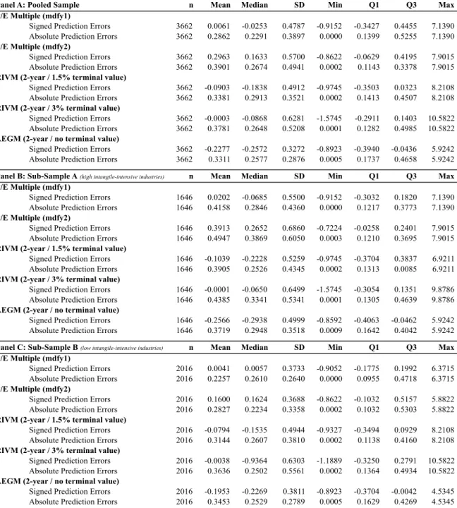
The descriptive statistics of valuation errors for each the selected valuation models and sub-sample is summarized next.

Table 4 - Descriptive statistics of valuation errors (trimmed data)

Panel A: Pooled Sample n Mean Median SD Min Q1 Q3 Max P/E Multiple (mdfy1)

Signed Prediction Errors 3662 0.0061 -0.0253 0.4787 -0.9152 -0.3427 0.4455 7.1390 Absolute Prediction Errors 3662 0.2862 0.2291 0.3897 0.0000 0.1399 0.5255 7.1390

P/E Multiple (mdfy2)

Signed Prediction Errors 3662 0.2963 0.1633 0.5700 -0.8622 -0.0629 0.4195 7.9015 Absolute Prediction Errors 3662 0.3901 0.2674 0.4941 0.0002 0.1143 0.3378 7.9015

RIVM (2-year / 1.5% terminal value)

Signed Prediction Errors 3662 -0.0903 -0.1838 0.4912 -0.9745 -0.3503 0.0323 8.2108 Absolute Prediction Errors 3662 0.3381 0.2913 0.3521 0.0002 0.1413 0.4507 8.2108

RIVM (2-year / 3% terminal value)

AEGM (2-year / no terminal value)

Signed Prediction Errors 3662 -0.2277 -0.2572 0.3272 -0.8923 -0.3940 -0.0436 5.9242 Absolute Prediction Errors 3662 0.3311 0.2577 0.2876 0.0005 0.1737 0.4658 5.9242

Panel B: Sub-Sample A (high intangile-intensive industries) n Mean Median SD Min Q1 Q3 Max P/E Multiple (mdfy1)

Signed Prediction Errors 1646 0.0202 -0.0685 0.5500 -0.9152 -0.3032 0.1820 7.1390 Absolute Prediction Errors 1646 0.4158 0.2846 0.4360 0.0000 0.1217 0.3773 7.1390

(31)

Mean and median valuation errors are tested for their statistical significance by applying parametric and non-parametric tests. Specifically, the t-test and the

Wilcoxon signed rank test are performed to test mean and median equality respectively. The results of these tests are presented in table 5 within all samples (pooled and sub-samples). A significance level of 5% is used for the hypothesis of both tests.

The hypotheses applied for the three samples in the t-test are the following: !! ∶ !"#$ !!"#!$%&' !""#" = 0

!_! ∶ !"#$ !"#$"%&'( !""#" ≠ 0

Regarding the Wilcoxon signed rank test, the hypotheses tests used are stated below: !_! ∶ !"#$%& !"#$"%&'( !""#" = 0

!! ∶ !"#$%& !"!"#$%&' !""#" ≠ 0

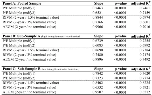
Table 5 – Intra-sample valuation accuracy and bias

Mean p-value Median p-value Mean p-value Median p-value P/E Multiple (mdfy1) 0.0061 0.3928 -0.0253 0.2594 0.2862 <0.0001 0.2291 <0.0001 P/E Multiple (mdfy2) 0.2963 <0.0001 0.1633 <0.0001 0.3901 <0.0001 0.2674 <0.0001 RIVM (2-year / 1.5% terminal value) -0.0903 <0.0001 -0.1838 <0.0001 0.3381 <0.0001 0.2913 <0.0001 RIVM (2-year / 3% terminal value) -0.0003 <0.0001 -0.0868 <0.0001 0.3781 <0.0001 0.2648 <0.0001 AEGM (2-year / no terminal value) -0.2277 <0.0001 -0.2572 <0.0001 0.3311 <0.0001 0.2577 <0.0001

Mean p-value Median p-value Mean p-value Median p-value P/E Multiple (mdfy1) 0.0202 0.2892 -0.0685 0.4561 0.4158 <0.0001 0.2846 <0.0001 P/E Multiple (mdfy2) 0.3913 <0.0001 0.2652 <0.0001 0.4947 <0.0001 0.3869 <0.0001 RIVM (2-year / 1.5% terminal value) -0.1039 <0.0001 -0.2228 <0.0001 0.3905 <0.0001 0.2526 <0.0001 RIVM (2-year / 3% terminal value) -0.0001 0.0456 -0.0650 0.0919 0.4385 <0.0001 0.3341 <0.0001 AEGM (2-year / no terminal value) -0.2566 <0.0001 -0.2938 <0.0001 0.3719 <0.0001 0.2948 <0.0001

Mean p-value Median p-value Mean p-value Median p-value P/E Multiple (mdfy1) 0.0041 0.9892 0.0057 0.6561 0.2257 <0.0001 0.2610 <0.0001 P/E Multiple (mdfy2) 0.1600 <0.0001 0.1624 0.0001 0.2827 <0.0001 0.2234 <0.0001 RIVM (2-year / 1.5% terminal value) -0.0794 <0.0001 -0.1535 <0.0001 0.3144 <0.0001 0.2607 <0.0001 RIVM (2-year / 3% terminal value) -0.0038 0.5621 -0.9364 0.9189 0.3636 <0.0001 0.2502 <0.0001 AEGM (2-year / no terminal value) -0.1953 <0.0001 -0.2269 <0.0001 0.3453 <0.0001 0.2529 <0.0001 Signed Prediction Errors Absolute Prediction Errors Panel A: Pooled Sample

Panel B: Sub-Sample A (high intangile-intensive industries)

Panel C: Sub-Sample B (low intangile-intensive industries)

Signed Prediction Errors Absolute Prediction Errors

Table 5 reports the results for both parametric (t-test) and non-parametric (Wilcoxon signed rank) tests within the respective samples and for all models. These tests were conducted at a significance level of 5%. Thus, a p-value below 5% indicates a statistically significant lack of valuation accuracy or/and significant biased valuation.

(32)

Regarding valuation bias, it is possible to conclude the models’ tendency to under- or overvalue. The results stated on table 5 show that P/E (1-year-ahead earnings) for all samples and RIVM (3% continuous growth9) for the two sub-samples do not result in a statistically significant mean bias, which means that models do not tend to either under- or overvalue.

When focusing on the stock- versus flow-based valuation models, there is an overall predisposition for flow-based valuation models to undervalue since mean valuation errors result in negative numbers. The tendency for flow-based models to undervalue in the sub-samples is relatively constant with a mean bias of -7.94% to -10.36.% for the RIVM (1.5% continuous growth10) and a higher bias for the AEGM of 19.53% to -25.66%. Accordingly, the AEGM shows the highest signed mean valuation errors. Flow-based models result in equally biased value estimates regardless industrial allocation. Industry differences become apparent when focusing on P/E multiple. Bias is significantly higher for high intensive industries compared to low intangible-intensive industries, which, in the case of the P/E (mdfy1), is the second smallest bias of the sample. In addition, P/E multiples indicate a slightly overvaluation, which is consistent with Liu et al. (2007). According them, multiple valuations result in positive bias, based on industry matching.

Concerning valuation accuracy, all models result in statistically significant mean absolute valuation errors, demonstrating a relevant lack of accuracy. Even though, there are relevant differences when focusing on each model separately.

P/E (1-year-ahead earnings) is the model with the lower accuracy value in the low intangible-intensive industries, with 22.57% of mean valuation accuracy followed by P/E multiple (2-year-ahead earnings) with 28.27% . Sub-sample A, on the contrary, has flow-based valuation models giving the lowest mean absolute valuation by missing, on average, 37.19% and 39.05% of price at valuation date, respectively for AEGM and RIV (1.5%). Comparing the two RIV models, the model with an inferior continuous growth (1.5%) outperforms its 3% alternative.

9

For the sake of simplicity, from now on, stated as 3%

10

(33)

Sub-sample A does not reveal similar results vis-à-vis sub-sample B, while P/E multiple reveals to be the superior model for sample B, AEGM is the outperformer model for sub-sample A. For the low intangible-intensive industry the 1-year-ahead P/E shows the least lack of accuracy, demonstrating that valuation performance, in this sub-sample, increases with the extension of the forecast horizon (Liu et. al (2002, 2007) and Lie and Lie (2002)). The AEGM is, again, the best flow-based model in terms of absolute valuation errors for high intangible-intensive firms. This fact can be explained by the increasing complexity of valuing intangible-intensive firms, which demands for more complex and comprehensive valuation models (Koller et al., 2005).

The larger valuation errors indicated by high intangible-intensive industries can be justified by higher volatility, instability and uncertain future expectation concerning these industries. According to Gu and Wang (2005), the superior information complexity of intangible assets increases the difficulty to assimilate information, which, consequently, raises forecast error for sub-sample A.

In conclusion, stock-based valuation models show the best results for both accuracy and bias valuation errors when analyzing low intangible-intensive industries. On the other hand, high intangible-intensive industries result in a better performance when flow-based valuation models are applied.

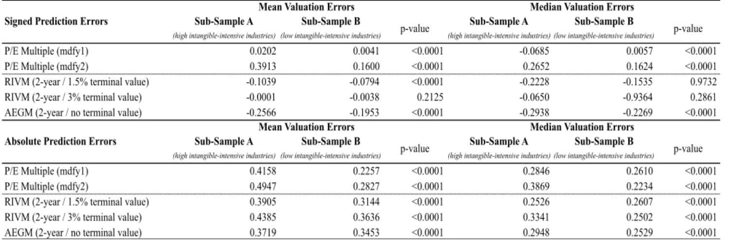
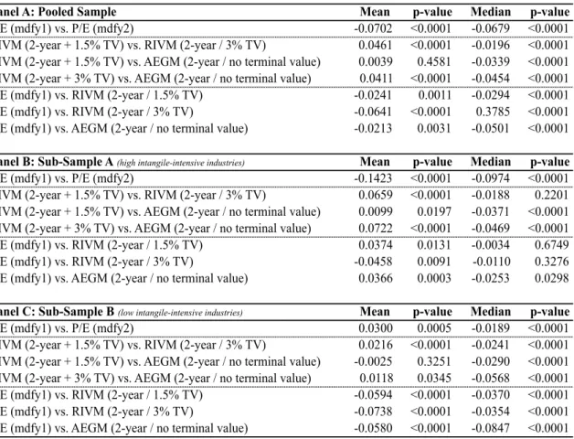
3.4.2.2 Cross-Sample Analysis of Valuation Errors

This section associates both sub-samples (A and B) to understand whether (or not) valuation models differ in bias and accuracy. Both parametric (two sample t-test) and non-parametric (Wilcoxon rank sum test) tests are conducted.

The hypotheses applied for the samples in the two sample t-test are the following: !_! ∶ Mean valuation error_{!!"! !"#$"%!&'(} = Mean valuation error_{!"# !"#$"%!&'(} !! ∶ Mean valuation error!!"! !"#$"%!&'( ≠ Mean valuation error!"# !"#$"%!&'(

Regarding the Wilcoxon rank sum test, the hypotheses tests used are stated below: !_! ∶ Median valuation error_{!!"! !"#$"%!&'(} = Median valuation error_{!"# !"#$"%!&'(} !_! ∶ Median valuation error_{!!"! !"#$"%!&'(} ≠ Median valuation error_{!"! !"#$"%!&'(}