MESTRADO MASTER IN FINANCE
TRABALHO FINAL DE MESTRADO
DISSERTAÇÃO
SIZE ANOMALIES IN E.U.BANK STOCK RETURNS
JOÃO PEDRO GROSSINHO REIS
MESTRADO EM MASTER IN FINANCE
TRABALHO FINAL DE MESTRADO
DISSERTAÇÃO
SIZE ANOMALIES IN E.U.BANK STOCK RETURNS
JOÃO PEDRO GROSSINHO REIS
ORIENTAÇÃO:
PROF.PEDRO NUNO RINO CARREIRA VIEIRA
1 Abstract
Recent studies have showed evidence of an existence of a size effect to be accounted for when computing the expected returns of a stock.
In commercial banks across the Euro monetary union, this effect is not clear. The returns on portfolios sorted by size do not favor in a big manner none of the size sorted portfolios but show a slight tilt in favor of the smallest portfolios.
We addressed the five factor Fama & French model and analyzed the returns by portfolio for this matter.
In comparison with the non-financial companies we also could not set a big difference between them. In the end we showed that the size effect needs to be studied in a deeper level and interpreted carefully.
2 Resumo
Em anos recentes tem-se gerado discussões em volta da existência e influência do fator “tamanho” nos retornos das ações de mercado. O modelo de capital asset princing (CAPM), propõe uma relação direta entre o risco de mercado e o retorno do ativo. Enquanto os resultados dos testes diretos a esta proposta não saem conclusivos, evidências recentes sugerem a existência de fatores adicionais a ter em conta aquando do cálculo do preço de uma ação. Litzenberger e Ramaswamy (1979) mostram uma relação positiva entre o price-earnings ratio e os retornos esperados das ações não financeiras. Basu (1977) encontra uma relação entre book-to-market ratio e os retornos esperados. Já em 1992, Fama e French mostram evidências de que existe um fator relacionado com o tamanho que tem que se ter em conta a quando da avaliação de ações. Todos estes autores vêm propor a existência de um modelo melhor para avaliar ações de mercado do que o CAPM. Gandhi e Lusting (2015) são os primeiros autores que vêm documentar e desvendar este fator “tamanho” a ter em conta nos bancos comerciais para o mercado dos Estados Unidos da América. O nosso trabalho vem tentar desvendar e elucidar um pouco mais este fator tamanho a ter em conta para bancos comerciais, deste modo para o mercado Europeu. Nós seguimos os modelos e métodos utilizados por Gandhi e Lusting assim como Fama e French. Fomos construir portefólios do mais pequeno para o maior e correr regressões para avaliar os seus retornos. O resultado deste estudo é menos expressivo do que o resultado obtido pelos autores Gandhi e Lusting para o mercado Americano. No entanto, é possível ver uma ligeira tendência para que os portefólios constituídos pelos bancos mais pequenos, tenham retornos superiores aos portefólios constituídos por grandes bancos.
3 Acknowledgements
First and foremost I want to thank my professor Pedro Rino Vieira for all the motivation and confidence he has given to me in order to be able to finish and present this paper.
This outcome would not be possible without him.
I also want to thank my family for all the support and comprehension I needed in times where only family could help me go forward.
Moreover, I cannot forget my friends that helped me not to quit and keep me on track of my goal.
I would like to give a special thanks to my friend Pedro Melo for hearing my problems and obstacles during this journey and always be able to help me clear some ideas. Likewise, to my sister Catarina for being an inspiration to follow.
4 Contents Introduction ... 5 1. Literature Review ... 6 2. Methodology ... 16 a. Playing field ... 16 b. Regression ... 17
3. Results and outputs... 19
4. Conclusion and Suggestion ... 25
References ... 28
5 Introduction
In recent years there has been an argument about the existence and influence of the size effect in stock returns. The capital asset pricing model (CAPM) presupposes a simple linear relationship between the expected return and the market risk of a security. While inconclusive test results from this relationship, recent evidence suggests an existence of additional factors relevant for asset pricing. Litzenberger and Ramaswamy (1979) show a positive relationship between price-earnings ratio and expected returns of common stocks. Basu (1977) finds that book-to-market ratio and expected returns are related. Fama and French (1993) show evidence of an inverse relationship between market value and common stock returns as well as a positive relationship with book-to-market ratio. All these authors came to propose an existence of better model to compute expected returns for common stock. Gandhi and Lusting (2015) are the first authors to document a size effect to be accounted for, when computing stock returns for commercial banks on the United States of America market. The size effect has become theme of discussion in the recent years and especially on commercial banks. Our work comes in order to help to have a better understanding of this size effect and its real existence on commercial banks. We decided to uncover the existence of a size effect on commercial banks for the European monetary union market, with the purpose of adding one more piece of the puzzle on size effects for commercial banks. For us to document the existence of the size factors we followed the same process used by Gandhi and Lusting, and also by Fama and French. Small banks tend to earn abnormal excess returns when ranked by market value. Assuming a buying and selling strategy; going long on the smallest portfolio and short on the largest (by market value), would give abnormal returns of 2,3% per month. Investing only on the smallest would earn 0,1% per month
6
whereas investing only on the largest would earn -2% per month. Also, the market beta is smaller for smaller firms by book value and market value (0,491 and 0,318), whereas for the largest firms is bigger (1,071 and 1,045), leading us to believe that largest commercial banks have higher market risk. In the next sections we will present the previous study in detail, the methodology and the results.
In section 1, we will present the context of our work, the work developed so far by other authors on the subject and the derivation of this paper. In section 2, we will show the data used, the methodology and the basis of the work following. In section 3, we show the results and outputs of the work developed. And finally, in section 4, we will conclude with some explanations, suggestions and work to follow.
1. Literature Review
Since the findings by Banz (1981) and Reinganum (1981) providing evidence that small size firms of common stock (small market capitalization) tend to earn, on average, higher risk adjusted returns than large size firms, that a lot of attention has been given to the size phenomenon. In his work, Banz (1981) suggests that the CAPM is miss-specified. He argues that there is an inverse relation between firm size and the average returns between 1936-1977 period and thus there is a size effect to be accounted for on the asset pricing model. However, it is difficult to determine if it is the market value per se that matters or if it is just a proxy for an unknown additional risk factor that needs be accounted for in the equilibrium pricing model (Banz, 1981). In other words, it is still to uncover if is the raw market value of the firm that impacts the company´s stock returns, or if this market value hides some kind of risk. Reinganum (1981) also argues that the
7
CAPM may lack significant empirical content since after testing for the relevance of Betas in the pricing model, he found that variations in estimated market betas are not systematically related to variations on average returns. He points that for the 1964-1979 period, average returns on high beta stocks are not consistently different from average returns of low beta stocks, and even low beta stocks show higher average returns when compared with high beta stocks for the 1964-1979 period tested, roughly the same period that Banz (1981) reported the size anomalies on common stock returns. In 1983, Basu corroborates the findings of a size effect by Banz, attributing the expected returns to the earning´s yield factor rather than to the size of common stocks. In line with Banz (1981), the author documented the same inverse relation between market value and adjusted returns. He also finds that firms of common stock with high Earnings/Price ratios earn, on average, higher risk-adjusted returns than firms with low Earnings/Price ratios. Such results support the hypothesis of a misspecification of the equilibrium pricing model, at least for the period studied of 1963-1979.
Keim (1983) reports the same size anomalies found by early authors for the same period of time (1963-1979) and makes the claim that these anomalous abnormal returns have more meaning in January relative to the remaining eleven months of the year. He confirms the negative relation between returns and size and shows that this relation is due in large scale to the January effect and even more to the first week of the month (50%), particularly on the first trading day of the year. Keim points out some reasons explaining this January effect (i.e tax loss selling or information releases by companies) but does not provide empirical support to them and leaves it to future studies. By then there were strong evidences that there was in fact a size effect and a misspecification of the asset pricing model or in the latter case, market inefficiency. Authors like
8
Rosenberg, Reid and Lanstein (1985) argue that prices on NYSE for the period of (1973-1984) may be inefficient according to their studies. They found that strategies consisting in buying stocks with a high book value of common equity per share to market price per share and selling stocks with low book/price ratio would earn abnormal returns, attributing this effect to market inefficiency. On the other hand Bhandari (1988) evidenced a positive relation between expected returns on common stock and the debt/equity ratio. The author also says that if the leverage effect found through the ratio is just a proxy for risk, then, a measure of risk different from the market beta, needs to be used. In any case, the evidence presented by Bhandari is also a test for the capital asset pricing model (CAPM) validity. In this case, the results show that a better model is needed, or at least, a better CAPM. Chan and Chen (1988) on the other hand argued that this size effect must arise from either a misspecification of this effect or substantial errors in estimating betas of the tested portfolios. Chan and Chen tested the second hypotheses in their work. They found that when estimating the betas using the same method as Banz (1981), using five years of past data, the results come consistent with Banz (1981). However, when the betas are estimated using a longer period of time, the results come different, eliminating the explanatory power of the size effect of the cross-sectional returns. These findings made Chan and Chen conclude that the imprecision in estimating the market beta in previous studies originated spurious results. Contradicting this theory, Jegadeesh (1992) tests the validity of the studies performed by Chan and Chen and uses the same procedures plus two additional sets of test portfolios that are constructed to have low cross-sectional correlation between beta and the size factor. Jegadeesh (1992, pp. 349) argues that it is difficult to “unambiguously attribute the differences in average returns to size or beta when these variables are highly correlated”
9
and after testing with different sets of portfolios and estimation beta models, he concludes that the market beta “do not explain the cross-sectional differences in average returns”. Therefore, the size effect can´t be explained by the market Beta, which justifies its need to be clarified. In order to address the asset-pricing misspecification, Fama and French (1993) tested common risk factors between stocks and bonds using the Arbitrage Pricing Theory as a base model. They tested the explanatory power of four additional factors, more precisely the most traditional ones in the CAPM, documented in previews works, Size, Earnings/Price, Leverage and Book/Market for stocks [see Banz (1981), Basu (1983), Bhandari (1988) and Rosenberg et al. (1985)] and other two factors for bonds, changes in interest rates and default. The authors found that “used alone or in combination with other variables”, the market beta, “has little information about average returns”. “Used alone, Size, E/P, Leverage and book-to-market equity have some explanatory power. In combination, Size and book-to-book-to-market equity seem to absorb the apparent roles of Leverage and E/P in average returns (Fama and French, 1993, pp. 4). The bottom-line is that Size and book-to-market equity do a good job explaining the cross-section of average returns on NYSE, AMEX and NASDAQ common stocks for the 1963-1990 period. Fama and French use SMB, HML and RMO as proxy´s for risk factors for stocks, representing the Size effect, book-to-market effect and the book-to-market premium respectively, and TERM and DEF for bonds, representing the changes in interest rates and default respectively. They found that constructing a five factor asset pricing model with three stock factors and two bond factors do a good job explaining common variation in bond and stock returns as well as the cross-section of average returns, these findings are very important for the work developed. By now there is a lot of literature pointing for a misspecification of the asset
10
pricing model related to a size effect and other measures of value, but the “why” is still a controversial theme. Lakonishok, Shleifer and Vishy (1994), henceforth LSV, once again show that value stocks (high B/M, E/P and small size stocks) tend to perform better than glamour stocks (Low B/M, E/P and big size stocks) and give some further light on why value strategies perform better than glamour strategies. They define Contrarian strategies as investments in low past growth and low future expected growth using a high (low) Cash flow/Price (E/P) as a proxy for a low (high) expected return. LSV also explore the claim by Fama and French (1992) that Value strategies are fundamentally riskier. The authors say that, in order “to be fundamentally riskier, value stocks must underperform glamour stocks with some frequency, and particularly in the states of the world when the marginal utility of wealth is high” (Lakonishok et al., 1994, pp. 1543). LSV find that this does not happen and thus, there is little, if any, support for value strategies to be fundamentally riskier. Explaining one of the reasons why contrarian strategies perform better than naive strategies (Extrapolation strategies) resides in the fact that individual investors and institutional money managers tend to look at the past high growth of stocks and extrapolate to future expected returns, making this type of stocks overpriced and value stocks underpriced. Another explanation not tested by the authors, has to do with the short-term horizons for both individual and institutional investors. As LSV reveal, in order to earn abnormal returns with value strategies, the investors need a 3 to 5 year horizon. This conclusion presents a divergence with the way in which individual investors tend to act, as they always look for fast returns (few months). The same occurs with institutional investors, who constantly need to show results to their sponsors in order to keep their jobs. Furthermore, the investors may not be aware of Contrarian strategy phenomenon. The
11
reasons for the size effect and other value measures in stock returns reported in previous works were studied by other authors. Kothari, Shanken and Sloan (1995) point to a selection bias on the COMPUSTAT data. Most authors, in previous works, use the COMPUSTAT platform to get the data to address the size effect. Kothari et al. (1995) suggest that the selection bias comes from a major COMPUSTAT data expansion occurred in 1978, where mostly surviving firms’1 data were included. Furthermore, “even in recent years, there are many firms with stock returns on the Center for Research in Securities Prices (CRSP) tapes, but financial data missing on COMPUSTAT” (Kothari et al., 1995, pp. 187). Almost simultaneously, Chan, Jegadeesh and Lakonishok (1995) contradict these findings, arguing that the sample selection bias on COMPUSTAT, if any, is trivial and exaggerated, and shouldn´t lead to big differences in returns. Also Barber and Lyon (1997) give some strength on the findings by Chan et al. (1995) since, in combination with Davis (1994) and Chan, Hamao and Lakonishok (1991) that studied the same impact of size and book-to-market effects in returns, for a different period of time and different country. They found no relevant evidence of survivorship-bias2 and data-snooping3 bias in the COMPUSTAT data that could affect dramatically the estimates for these factors, and thus the results of Fama and French (1993), suggested by Kothari et al. (1995). The authors also enhance the weakening of the survivorship and snooping-data bias. In any year of the sample, they were able to reject the null-hypothesis that, the size or book-to-market premium, differ between financial and nonfinancial firms. These conclusions corroborate once more the findings by Fama and French on the explanatory power of size and
1 Surviving firms are the ones that, according to the COMPUSTAT standards, are selected be a part of
the data; non-delisted and meeting the minimum asset or market value requirements.
2 Process of selecting things or people, in this case firms, which “survived” a selection process,
overlooking those that did not.
12
market on returns of common-stock. Despite the consistency of the Fama and French factors and the growing empirical support, there is always a controversy relative to the explanatory power of the factors found. Daniel and Titman (1997) argue that it is the firm´s characteristics rather than factor loadings that determinate expected returns. The authors say that relative distress drives stock returns, and B/M is a proxy for distress. Also firms with similar characteristics (like size and B/M) tend to enter in distress phases at the same time. In response to this theory, Davis, Fama and French (2000) tested the same methods used by the previous authors but extended the data (1929-1997 against 1973-1993) and found that the results from Daniel and Titman were period specific. In the sequence of the findings by (Fama and French, 1998, pp. 1997) that “value stocks tend to have higher returns than growth stocks in markets around the world”, Griffin (2002) tried to find the factor model that better explains time-series variation in international stock returns. Griffin tested the explanatory power of a domestic, world and international three-factor model from Fama and French (1993). He found that, for the full sample (1981-1995) and later period (1990-1995) the regressions results show that the domestic three-factor model has greater explanatory power and in most cases lower pricing errors than the world three-factor model. In the case of the international three-factor model, the intercepts that are farther from zero than the domestic models, indicating the presence of foreign factors, do not lead to a better pricing. In addition, the world and international models produce a less accurate forecast than the domestic three-factor model for returns. Likewise, Fama and French (2006) when trying to show the robustness of their findings on value premium relative to size and the explanatory power of CAPM, with an out-of-sample test, they found evidence for international value premiums on 14 major markets outside the United States for the
13
period 1975-2004. In a recent paper, Fama and French (2012) find once more evidence of value premiums in average returns in four regions (North America, Europe, Japan and Asia Pacific). Similarly, they found strong momentum returns in all regions except Japan. For this matter they “tested whether value and momentum patterns in average returns are captured by empirical asset pricing models across regions” (Fama and French, 2012, pp.2). They examined how well global and region specific models, CAPM, Three-factor and four-factor model (taking momentum into consideration), capture average returns. In this paper the authors claim that global models do a poor job explaining the regional size-B/M portfolios, local three-factor models are quite passable for average returns on size-B/M portfolios in Japan and Europe and that nothing is added or lost in adding the momentum factor (four-factor model). When evaluating the global four-factor model, the authors say that it is acceptable for a global size-momentum portfolio but it performs poorly on regional size-size-momentum portfolios. The bad specification of local size-momentum comes from Asia Pacific and Europe. In the European case, the four-factor model comes rejected for the European size-momentum returns. Nonetheless Fama and French are comfortable in using the four factor-model when explaining returns of a global portfolio (i.e a mutual fund with global stocks) as long as the portfolio does not have a strong bias towards micro caps or stocks from a particular region.
“Banks are much different from non-financials in many ways”, the “most salient distinction is that banks are subject to bank runs4 during panics and crises, not just by depositors but also by other creditors” (Gandhi and Lusting, 2015, pp. 2). Gordon and Metrick (2012) and Duffie (2010) illustrate how these runs occur and how they impact
4 Bank runs represent the rush from costumers to commercial banks in order to withdraw cash and close
14
the banks liquidity. The liquidity dry-out and consequent bankruptcy is due to a chain of events. Both authors say that, nowadays, the banking system has changed. “Dealer banks” (securitized banking5) are playing an increasing role alongside with traditional banking6 (commercial banking), acting as both. In that scenario, bank runs related to the securitized banking strongly impacts commercial banking leading to runs on commercial banks as well. There are two types or bank runs, a traditional-banking run which is driven by the withdrawal of depositors and a securitized-banking run which is driven by withdrawal of repo agreements (Gordon and Metrick, 2012). In the recent crises of 2008, Gordon and Metrick argue that a run on the “securitized-banking” related to the prime mortgage and repo collaterals, was the trigger to the illiquidity of the banking system where banks couldn’t honor their demands to costumers. Since “financial crises are high marginal utility states for the average investor, the expected return on bank stocks should be specially sensitive to a variation in the anticipated financial disaster recovery rates of bank´s shareholders related to bank size, the regulatory regime, implicit government guarantees, and other characteristics” (see Gandhi and Lusting, 2015, pp. 2). “Dealer banks” (securitized banking) are often parts of large complex financial organizations whose failures can damage the economy significantly. As a result, they are sometimes considered “too big to fail” (Duffie, 2010). In this context, if a bank is “too big to fail”, the expected returns on its stock should be, in equilibrium, lower since, in some cases, governments absorb some of the largest bank´s tail risk. In this line of the thinking, Gandhi and Lusting (2015) studied the size effect of the balance sheet on bank stock returns and not just only the market value.
5 Firms formerly known as investment banks (e.g Lehman Brothers, Morgan Stanley, Merrill Lynch)
(Gorton and Metrick, 2012).
6 “Business of making and holding loans, with insured demand deposits as the main source of funds.”
15
Their paper is the first to document that the firm size on financial stocks is really about size and not about market capitalization. They found that “the largest commercial bank stocks, ranked by total size of the balance sheet, have significantly lower risk-adjusted returns than small- and medium-sized bank stocks, even though large banks are significantly more levered” (see Gandhi and Lusting, 2015, pp. 1). This size effect is relative to book value and not to market capitalization documented by earlier authors. Gandhi and Lusting contribute a great deal in uncovering the size effect in financial stocks by constructing a size factor to be accounted for on the asset pricing model. Since large banks are more leveraged and more exposed to the market risk (large banks have higher betas than small banks) the risk-adjusted returns shouldn´t be much different from small banks “unless there is a bank-specific tail risk priced but not spanned” “consistent with government guarantees that protects shareholders of large, but not small banks, in disaster states” (Gandhi and Lusting, 2015, pp. 2). They attributed the size effect in financial stocks to how tail risk is priced and this tail risk premium is determined by the bank´s loading on the size factor. The size factor is based on a principal component analysis to study the common variation of the bank´s payoffs. “Firms that are deemed systematically important have negative loadings on this size factor because they are less likely to be allowed to fail, by government guarantees, in the event of a financial disaster” (Gandhi and Lusting, 2015, pp. 5). Previous authors did not incorporate financial stocks on their studies because they believed that the leverage effect would affect their results. Since there´s a lack of knowledge on the size effect relative to commercial bank stocks, my contributions help to uncover the size effect in the euro-zone.
16 2. Methodology
a. Playing field
For our study we selected commercial banks from the Eurozone7 to construct the portfolios. By doing this we made sure that all the banks in the sample are regulated by one single entity, the European Central Bank. Choosing a sample from the entire European Union would imply using banks with different currencies and different regulatory standards. We used Bankscope platform in order to gather the data. To follow the selection method used by Fama and French (1993) and Gandhi (2015), the banks must be active, listed, have positive book values and with at least two years of information. From this selection we ended up with 59 commercial banks that follow these criteria and thus eligible to test. Our sample takes in account 19 countries of the Eurozone since two of them entered in the last two years, Latvia and Lithuania, putting them out of the sample for the lack of information available. Also UK and Switzerland are not part of the EU and thus do not make our test. The test sample for this study covers 70,3% of operating income and 67% of total assets in all European Union commercial banks (Bankscope). We started our data from 01/01/2000 since information like Book value in some cases is updated annually and the euro was only introduced on 01/01/1999. Similarly to previous authors, we collected monthly data, ended up with monthly returns, market values and book values for the last 15 years. The non-financial companies where obtained from DataStream platform. We gathered 1247 non-financial companies from all the main and secondary exchange markets for the countries in the study. We performed the same filters as in the previous group and ended up with
7 Eurozone is composed by; Germany, Austria, Belgium, Cyprus, Slovakia, Slovenia, Spain, Estonia,
Finland, France, Greece, Republic of Ireland, Italy, Latonia, Latvia, Luxemburg, Malta, Holland and Portugal.
17
monthly returns, market values and book values for the last 15 years as well. We then constructed the portfolios by grouping the stocks by size of market cap and book value in deciles. Meaning that the portfolio number one would be composed by the ten percent smallest stocks by size, market cap at first and then book value. Each year we have ten portfolios per month, making it 1800 portfolios to run the regression.
b. Regression
In order to adjust the portfolio returns for exposure to the standard risk factors that explain cross-sectional variation in average returns on other portfolios of nonfinancial stocks and bonds we use the Fama and French three factor-model in accordance with Gandhi (2015). Like in Gandhi´s paper, we use the three factor model and also include two bond risk factors since we can see the core business of commercial banks as managing a portfolio of bonds of varying maturities and credit risk. The explanatory variables in the time series regression include market return, small minus big, high minus low and the two bond factors.
𝑓𝑡 = [ 𝑚𝑎𝑟𝑘𝑒𝑡 𝑠𝑚𝑏 ℎ𝑚𝑙 𝑙𝑡𝑔 𝑐𝑟𝑑 ]
The terms 𝑚𝑎𝑟𝑘𝑒𝑡, 𝑠𝑚𝑏, and ℎ𝑚𝑙 represent returns on the three Fama-French factors on stock returns. We capture 𝑚𝑎𝑟𝑘𝑒𝑡 by using the Datastream European monetary union stock index returns and subtracting the German one-month Treasury bill rate8. Both returns were withdrawn from Thomson Reuters Datastream platform. In order to get the 𝑠𝑚𝑏 and ℎ𝑚𝑙 returns we used the Fama&French construction method, we sort
8 We use the German Treasury bill as risk free rate since it´s close to the Euro area yield curve based
18
stocks into two market cap groups and three book-to-market equity groups. We then constructed a six value-weighted (two-dimensional) portfolios. 𝑠𝑚𝑏 is the equal-weight average of the returns on the three smallest stock portfolios for the region minus the average of the returns on the three bigger stocks portfolios9. ℎ𝑚𝑙 is the equal-weight average of the returns for the two high B/M portfolios for a region minus the average of the returns for the two low B/M portfolios10. The size factor or 𝑠𝑚𝑏 factor “Small minus Big” measures the return differential between the average small cap and the average big cap portfolios, while the book-to-market factor or ℎ𝑚𝑙 factor “High minus Low” measures the return differential between the average value and the average growth portfolios11. We use 𝑙𝑡𝑔 to denote the excess returns on a 10-year Government bond index for the Euro monetary union drawn from DataStream platform. We use 𝑐𝑟𝑑 to denote the excess returns on the Iboxx Euro monetary union corporate bond index downloadable from Datastream. The excess returns are computed based on our risk-free rate, the German one-month T-bill. Having all the variables we are able to regress the monthly excess returns for each size sorted portfolio on the Fama-French three stock factors and two bond factors. For each 𝑖 portfolio we run the following time series regression in order to estimate the vector of the betas 𝛽𝑖.
(1) 𝑅𝑡+1𝑖 − 𝑅𝑡+1𝑓 = 𝛼𝑖 + 𝛽𝑖,´𝑓𝑡+1+ 𝜀𝑡+1𝑖 ,
9 SMB = 1/3 (Small Value + Small Neutral + Small Growth) – 1/3 (Big Value + Big Neutral + Big
Growth).
10 HML = 1/2 (Small Value + Big Value) – 1/2 (Small Growth + Big Growth).
11 The Fama-French factors were computed based on the method used by them in previous works and
19 (2) 𝑅𝑡+1𝑖 − 𝑅𝑡+1𝑓 = 𝛼𝑖+ 𝛽𝑚𝑖 (𝑅𝑚− 𝑅𝑓) + 𝛽𝑠𝑚𝑏𝑖 (𝑅𝑠𝑚𝑏𝑖 − 𝑅𝑓) + 𝛽ℎ𝑚𝑙𝑖 (𝑅ℎ𝑚𝑙𝑖 − 𝑅𝑓) +
𝛽𝑙𝑡𝑔𝑖 (𝑅𝑙𝑡𝑔𝑖 − 𝑅𝑓) + 𝛽𝑐𝑟𝑑𝑖 (𝑅𝑐𝑟𝑑𝑖 − 𝑅𝑓) + 𝜀𝑡+1𝑖 ,
3. Results and outputs
Table I provides the results of the regression specified in equation (2) relative to commercial banks in the European monetary union. The portfolios are ranked from smallest (1) to the largest (2) in terms of market value (market cap) and Book value. The table reports the regression coefficients for each size-sorted portfolio with 5% confidence level along with 𝑅2. Panel A reports the results based on sorting by market capitalization into deciles. The estimated intercepts do not assume a monotonically decrease but it is clearly noticeable an excess return on the smallest portfolios by market cap. The intercepts are positive for the first, second and forth portfolio, here we can see that the largest porfolios earn lower returns when compared with the smallest portfolios. Also when looking for the difference between the largest and smallest portfolio (10-1), the intercept is negative (–2,3%) at 5% confidence level, meaning that going long on the smallest portfolio and short on the largest would give a 2,3% excess returns. When we look at the 𝑚𝑎𝑟𝑘𝑒𝑡 factor the opposite happens. There isn´t a size tendency upwards or downwards but it is noticeable that larger firms tend to have higher market risk. On the other coefficients we cannot see a clear tendency. As for the variance of the dependent variable (𝑅𝑡+1𝑖 − 𝑅𝑡+1𝑓 ) the estimated variables explain better the bigger portfolios just by interpreting the 𝑅2, increasing from 0,122 to 0,797 on the 9th portfolio and then
20
0,366 on the 10th. By looking at the ANOVA output on the table III12 we can see that the significance level is 0, below 0,05, leading us to say that the model is significant for all portfolios and that the coefficients estimated by the regression are statistically different. Now testing the multicollinearity of the coefficients on table V, we won´t suspect of any multicollinearity problems since all of our VIF (variance inflation factor) is low and way below 5. On the Panel B, representing the portfolios size-ranked for book value on commercial banks, we can´t see a size tendency on the constant (α) or on the rest of the coefficients except for the 𝑚𝑎𝑟𝑘𝑒𝑡 factor that has bigger returns for larger firms at a 5% confidence level. As for the 𝑅2 we notice that the model is more significant for the largest firms as for panel A.
21 Table I
This table presents estimates from OLS regression of monthly value-weighted excess returns on each size sorted portfolio of Euro monetary union commercial banks on the three Fama and French (1993) stock and two bond risk factors. Market, smb, and hml are the three Fama-French stock factors: market, small minus big, and high minus low, respectively. ltg is the excess return on an index of long-term German government bond and crd is the excess return on an index of investment-grade corporate bonds. * indicate statistical significance at the 5% level. The sample is from 2000 to 2015 in Panel A and B. small 2 3 4 5 6 7 8 9 10 10-1 Panel A: Market Capitalization α 0,001 0,008 -0,008 0,007 -0,007 -0,004 -0,003 -0,002 -0,002 -0,02* -0,023* 0,381* 0,891* 0,865* 0,736* 0,727* 1,002* 1,167* 1,254* 1,034* 1,045* 0,674* 0,150 0,280* 0,213* 0,231* -0,016 0,220* 0,422* 0,521* 0,439* 0,031 -0,113 -0,081 -0,125 -0,145 -0,052 0,098 0,384* 0,090 0,332* 0,431* 0,101 0,172 -0,181 0,111 -0,061 -0,157 -0,004 -0,382 -0,220 -0,130 -0,166 1,517* -1,315 0,585 -0,334 0,982 -0,071 0,243 1,943* 0,941 0,023 0,332 2,999* 2,417* 0,121 0,365 0,362 0,353 0,263 0,555 0,678 0,791 0,797 0,366 0,198 small 2 3 4 5 6 7 8 9 10 10-1 Panel B: Book Value α -0,003 -0,003 0,00 -0,006 0,003 -0,005 -0,006 0,00 -0,003 -0,002 -0,002 0,491* 0,670* 0,677* 0,877* 1,155* 0,970* 0,913* 0,830* 0,923* 1,072* 1,072* 0,211* 0,035 0,187* 0,330* 0,666* 0,295* 0,325* 0,483* 0,545* 0,568* 0,568* -0,174 -0,187 0,025 -0,099 0,176* 0,545* 0,149 0,298* 0,432* 0,230* 0,230* -0,514 -0,176 -0,249 -0,299 -0,356 0,097 0,251 -0,084 -0,134 -0,424 -0,424 0,448 0,522 1,013* 0,373 0,435 -0,009 0,532 0,982* 0,325 0,348 0,348 0,122 0,312 0,368 0,421 0,616 0,590 0,666 0,735 0,839 0,859 0,859
22
Table I shows the coefficients and 𝑅2 for the regression based on portfolios ranked on size for market value and book value using only non-financial companies. The goal here is to compare with the commercial banks and record some kind of behavior as on Gandhi (2015). Panel A refers to the portfolios ranked on market value. Analyzing panel A we cannot see a clear tendency for the constant. The market beta shows the same behavior as for commercial banks, however this behavior is less noticeable. The returns on 𝑠𝑚𝑏 and ℎ𝑚𝑙 show a size propensity for the smallest companies since the excess returns are bigger on the first portfolios constructed on size of market cap. At the same time is clear that the model does a good job explaining the variability of the dependent variable. Panel B shows a slight size factor when portfolios are formed on book value. It is clear, at a 5% confidence level, that the constant for the first and smallest five portfolios is higher than the last five and largest portfolios. Also, the portfolio (10-1) shows that; by investing on the largest portfolio (10) and short-selling the smallest portfolio (1) we would earn negative returns of -0,9% per month, meaning that, by inverting this strategy we would get abnormal returns in the same percentage. Again, the market beta shows higher values for largest companies. As for 𝑠𝑚𝑏 and ℎ𝑚𝑙 they show higher intercepts for smallest firms. The ANOVA output on the table IV shows the same result for both panels, the significance levels are all 0 and the Z values are high, meaning that the coefficients are statistically different in between portfolios and the model is significant. The test for the multicollinearity on table VI shows that there is no evidence of multicollinearity between factors since the numbers for VIF are all low and below 5 for both panels. Table VII shows the results for the average comparison on independent samples by performing a T-test. We tested the difference on
23
average excess returns between each portfolio but the outputs on table V refer only to the smallest (1) and largest (10) portfolios since the results came similar and the main goal here is to compare the smallest and largest returns. When looking at Panel A of the table VII, we can see a difference on average returns between the two portfolios, and when looking at the significance level this comes higher than 0,05 and thus we can assume similar variances. From here we can assume that the difference in the average excess monthly returns of the portfolios is statistically plausible. Then is possible to say that the average returns from the smallest and largest portfolios are statistically different. The same conclusion we take from analyzing the panel B of the table VII, we can assume different average excess monthly returns.
24 Table II
This table presents estimates from OLS regression of monthly value-weighted excess returns on each size sorted portfolio of Euro monetary union non-financial stock firms on the three Fama and French (1993) stock and two bond risk factors. Market, smb, and hml are the three Fama-French stock factors: market, small minus big, and high minus low, respectively. ltg is the excess return on an index of long-term German government bond and crd is the excess return on an index of investment-grade corporate bonds. * indicate statistical signicance at the 5%,level. The sample is from 2000 to 2015 in Panel
A and B.
small 2 3 4 5 6 7 8 9 10 10-1
Panel A: Market Capitalization α 0,001 0,003 0,005* 0,008* 0,008* 0,007* 0,008* 0,008* 0,005* 0,003* 0,00 0,729* 0,813* 0,863* 0,835* 0,894* 0,877* 0,820* 0,887* 0,908* 0,872* 0,152* 0,610* 0,630* 0,639* 0,665* 0,651* 0,448* 0,379* 0,208* 0,098* -0,353* -0,957* 0,132* 0,042* 0,022 0,059* 0,020 0,007 -0,010 0,012 0,009 0,015 -0,122* 0,296 -0,133 -0,023 -0,080 -0,159 -0,143 -0,449* -0,230* -0,158 -0,087 -0,348* -0,049 0,298 0,313* 0,336* 0,284 0,557* 0,969* 0,613* 0,369* 0,11 0,135 0,712 0,851 0,898 0,891 0,897 0,886 0,875 0,894 0,902 0,937 0,599 small 2 3 4 5 6 7 8 9 10 10-1
Panel B: Book Value α 0,006* 0,007* 0,006* 0,005* 0,002 0,005* 0,001 0,002* 0,004* -0,001 -0,009* 0,689* 0,716* 0,849* 0,877* 0,866* 0,973* 0,905* 0,798* 0,915* 1,054* 0,368* 0,055* 0,020* 0,030* 0,025* -0,029* 0,019* -0,015* -0,011* 0,021 0,057 -0,008* 0,580* 0,641 0,604 0,596 0,753 0,502 0,444 0,330 0,103 -0,087* -0,656 0,287* 0,045 0,076 -0,171 -0,232* -0,178 -0,172 -0,418* -0,223 -0,041 -0,305 -0,359 0,082 0,082 0,249 0,402* 0,483* 0,429* 0,640* 0,668* 0,040 0,379 0,744 0,824 0,868 0,903 0,898 0,869 0,896 0,910 0,868 0,915 0,609
25 4. Conclusion and Suggestion
Our paper contributes on documenting size effects in commercial bank stock. After regressing the size ranked portfolios and performing the tests; we conclude that there is not a clear size effect in the Euro monetary union like the one documented by Gandhi for the U.S stock market. The results show a little tendency on favor of the small stocks. The excess returns on the smallest firms for the commercial banks are more visible on the Panel A relative to the market value. As for the excess returns in the non-financial companies this excess returns are more visible on Panel B relative to book value. If we only look for the difference between the largest portfolios and the smallest, both panels for commercial banks and panel B for non-financial firms show that this strategy leads to negative returns. This means that if we invert the strategy, and assuming a buying and selling strategy, going long on the smallest portfolio and short the largest we would earn 27% per year on commercial banks ranked by market cap and 2,4% per year ranked by book value. Following the same strategy we would earn 10,8% per year on financial firms ranked on book value. When comparing commercial banks and non-financial firms, only the market returns and small minus big are significant at 5% confidence level for commercial banks, whereas on the non-financial firms, market, small minus big and high minus low are significant at 5% level of confidence. Now when comparing between small and big related to market risk it is clear that the largest commercial banks have more market risk as we expect since they manage the worlds wealth and when there is a bank run the largest banks are the ones that suffer the most. This tells us that the factors used to replicate the maturity risk and credit risk are barely significant when using the model to compute returns and that the book value does take more part in the returns of non-financials. In conclusion there is a single size effect to be
26
accounted for both on commercial banks and non-financial firms for the Euro monetary union but the results don´t show a big and evident proof of that like in previous works. Big caution is needed when interpreting the results and choosing a strategy since the reasons behind the size effect are still to uncover and especially across markets and regulatory regimes.
This paper intended to create more knowledge related to the existing evidences on size effects. For this matter we tried to follow methodologies used and performed by previous authors in very important works. The reasons behind this size effect are very difficult to prove, despite the fact that Gandhi did a great job in order to uncover this size effect for banks. However there is still a big controversy about it. The suspicions unveiled with this paper is that this size effect is stronger on the North American stock market than in the European euro zone market. The size of the market is a factor to take in account when comparing the results and trying to get any explanation, as well as the liquidity and number of transaction per day of both markets. In the end, other fields, such as behavior and culture on finance, may significantly influence markets and thus these particular size effects. The fact that there are more players involved in stock trading in the U.S market may affect the awareness of certain stocks for instance; big, successful and well known firms are popular and more people are aware of them, making them a “sure thing” for investors, but in the other hand they may be overpricing this stocks ready to crash.
The limitations of the work performed are related to the lack of banks and differences in commercial bank sizes. In order to do a thorough work, as performed by Gandhi, the sample gets very restricted. In addition to that, there is a big difference in the commercial bank´s controller organization in both markets. Also, and to perform
27
adequately and to develop an efficient work, it is necessary to have an exquisite and professional tool, rather than a simple Excel worksheet, namely because we are dealing with giant data.
The work to be done here is to try to understand the reasons behind this size effect or to add more proof of this size effect for different types of markets and try to find a resemblance. We would suggest a comparison between regions of the same continent/country that have the same behavior towards the market.
28 References
1.Banz, R. (1981). The relationship between return and market value of common stocks. Journal of Financial Economics, 9(1), pp.3-18.
2.Barber, B. and Lyon, J. (1997). Firm Size, Book-to-Market Ratio, and Security Returns: A Holdout Sample of Financial Firms. The Journal of Finance, 52(2), p.875.
3.Basu, S. (1983). The relationship between earnings' yield, market value and return for NYSE common stocks. Journal of Financial Economics, 12(1), pp.129-156. 4.Berk, J. (1995). A Critique of Size-Related Anomalies. Review of Financial Studies,
8(2), pp.275-286.
5.Bhandari, L. (1988). Debt/Equity Ratio and Expected Common Stock Returns: Empirical Evidence. The Journal of Finance, 43(2), p.507.
6.Chan, K. and Chen, N. (1988). An Unconditional Asset-Pricing Test and the Role of Firm Size as an Instrumental Variable for Risk. The Journal of Finance, 43(2), p.309.
7.Chan, L., Jegadeesh, N. and Lakonishok, J. (1995). Evaluating the performance of value versus glamour stocks The impact of selection bias. Journal of Financial Economics, 38(3), pp.269-296.
8. Cheol, E. S. (1994). The benchmark Beta, CAPM, and Pricing Anomalies. Oxford Journals, 46(2), pp.330-343.
9.Daniel, K. and Titman, S. (1997). Evidence on the Characteristics of Cross Sectional Variation in Stock Returns. The Journal of Finance, 52(1), p.1.
10.Davis, J., Fama, E. and French, K. (2000). Characteristics, Covariances, and Average Returns: 1929-1997. SSRN Electronic Journal.
11.Duffie, D. (2010). The Failure Mechanics of Dealer Banks. Journal of Economic Perspectives, 24(1), pp.51-72.
29
12.Fama, E. and French, K. (1992). The Cross-Section of Expected Stock Returns. The Journal of Finance, 47(2), pp.427-465.
13.Fama, E. and French, K. (1993). Common risk factors in the returns on stocks and bonds. Journal of Financial Economics, 33(1), pp.3-56.
14.Fama, E. and French, K. (1998). Value Versus Growth: The International Evidence. SSRN Electronic Journal.
15.Fama, E. and French, K. (2006). The Value Premium and the CAPM. SSRN Electronic Journal.
16.Fama, E. and French, K. (2011). Size, Value, and Momentum in International Stock Returns. SSRN Electronic Journal.
17.Gandhi, P. and Lusting, H. (2015). Size Anomalies in U.S. Bank Stock Returns. The Journal of Finance, 70(2), pp.733-768.
18.Gorton, G. and Metrick, A. (2012). Securitized banking and the run on repo. Journal of Financial Economics, 104(3), pp.425-451.
19.Griffin, J. (2002). Are the Fama and French Factors Global or Country-Specific?. SSRN Electronic Journal.
20.Jegadeesh, N. (1992). Does Market Risk Really Explain the Size Effect?. The Journal of Financial and Quantitative Analysis, 27(3), p.337.
21.Jensen, G., Johnson, R. and Mercer, J. (1997). New Evidence on Size and Price-to-Book Effects in Stock Returns. Financial Analysts Journal, 53(6), pp.34-42. 22.Keim, D. (1983). Size-related anomalies and stock return seasonality. Journal of
Financial Economics, 12(1), pp.13-32.
23.Kothari, S., Shanken, J. and Sloan, R. (1995). Another Look at the Cross-section of Expected Stock Returns. The Journal of Finance, 50(1), pp.185-224.
24.Lakonishok, J., Shleifer, A. and Vishny, R. (1994). Contrarian Investment, Extrapolation, and Risk. The Journal of Finance, 49(5), p.1541.
30
25.Leledakis, G., Davidson, I. and Smith, J. (n.d.). Does Firm Size Predict Stock Returns? Evidence from the London Stock Exchange. SSRN Electronic Journal. 26.Reinganum, M. (1981). A New Empirical Perspective on the CAPM. The Journal of
Financial and Quantitative Analysis, 16(4), p.439.
27.Rosenberg, B., Reid, K. and Lanstein, R. (1985). Persuasive evidence of market inefficiency. The Journal of Portfolio Management, 11(3), pp.9-16.
28. Basu, S. (1977). Investment Performance of Common Stocks in Relation to Their Price-Earnings Ratios: A Test of the Efficient Market Hypothesis. The Journal of Finance, 32(3), p.663.
29. Litzenberger, R. and Ramaswamy, K. (1982). The Effects of Dividends on Common Stock Prices Tax Effects or Information Effects. The Journal of Finance, 37(2), pp.429-443.
31 Appendix
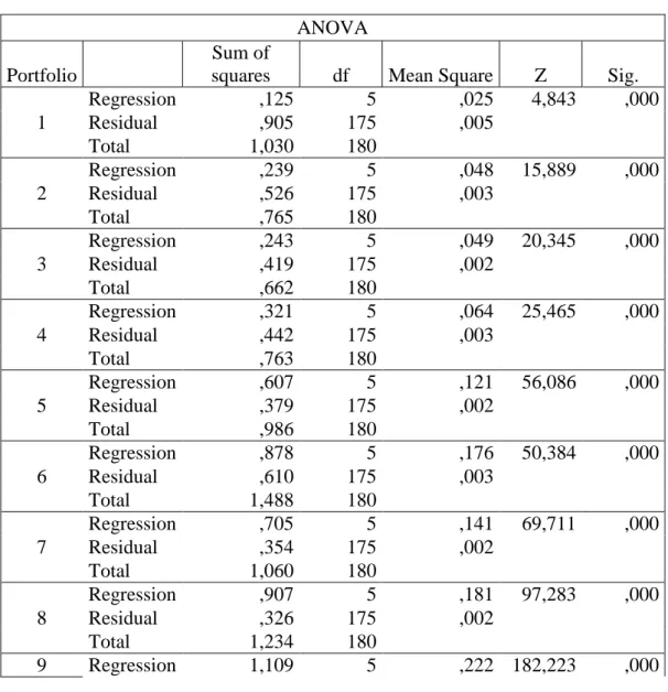
Table III
This table presents the ANOVA outputs of the regressions for the European monetary union commercial banks. The results are dived per size sorted portfolios formed on market value and book value. The samples is from 2000 to 2015 for panel A and panel B
Panel A
ANOVA Portfolio
Sum of
squares df Mean Square Z Sig.
1 Regression ,125 5 ,025 4,843 ,000 Residual ,905 175 ,005 Total 1,030 180 2 Regression ,239 5 ,048 15,889 ,000 Residual ,526 175 ,003 Total ,765 180 3 Regression ,243 5 ,049 20,345 ,000 Residual ,419 175 ,002 Total ,662 180 4 Regression ,321 5 ,064 25,465 ,000 Residual ,442 175 ,003 Total ,763 180 5 Regression ,607 5 ,121 56,086 ,000 Residual ,379 175 ,002 Total ,986 180 6 Regression ,878 5 ,176 50,384 ,000 Residual ,610 175 ,003 Total 1,488 180 7 Regression ,705 5 ,141 69,711 ,000 Residual ,354 175 ,002 Total 1,060 180 8 Regression ,907 5 ,181 97,283 ,000 Residual ,326 175 ,002 Total 1,234 180 9 Regression 1,109 5 ,222 182,223 ,000
32 Residual ,213 175 ,001 Total 1,322 180 10 Regression 1,225 5 ,245 212,387 ,000 Residual ,202 175 ,001 Total 1,426 180 (10-1) Regression 1,225 5 ,245 212,387 ,000 Residual ,202 175 ,001 Total 1,426 180 Panel B ANOVA Portfolio Sum of
squares df Mean Square Z Sig.
1 Regression ,071 5 ,014 4,804 ,000 Residual ,515 174 ,003 Total 0,586 179 2 Regression ,281 5 ,056 20,046 ,000 Residual ,488 174 ,003 Total ,770 179 3 Regression ,345 5 ,069 19,705 ,000 Residual ,609 174 ,003 Total ,953 179 4 Regression ,217 5 ,043 19,014 ,000 Residual ,398 174 ,002 Total ,615 179 5 Regression ,299 5 ,060 12,415 ,000 Residual ,837 174 ,005 Total 1,136 179 6 Regression 1,028 5 ,206 43,460 ,000 Residual ,823 174 ,005 Total 1,850 179 7 Regression 1,239 5 ,248 73,329 ,000 Residual ,588 174 ,003 Total 1,827 179 8 Regression 1,499 5 ,300 131,312 ,000 Residual ,397 174 ,002 Total 1,896 179 9 Regression 1,133 5 ,227 136,973 ,000 Residual ,288 174 ,002 Total 1,421 179 10 Regression 1,065 5 ,213 20,062 ,000
33 Residual 1,847 174 ,011 Total 2,911 179 (10-1) Regression 0,649 5 ,130 8,604 ,000 Residual 2,627 174 ,015 Total 3,276 179 Table IV
This table presents the ANOVA outputs of the regressions for the European monetary union non-financial companies. The results are dived per size sorted portfolios, formed on market value and book value. The samples is from 2000 to 2015 for panel A and panel B
Panel A
ANOVA Portfolio
Sum of
squares df Mean Square Z Sig.
1 Regression ,320 5 ,064 86,411 ,000 Residual ,130 175 ,001 Total ,450 180 2 Regression ,413 5 ,083 200,663 ,000 Residual ,072 175 ,000 Total ,486 180 3 Regression ,441 5 ,088 308,097 ,000 Residual ,050 175 ,000 Total ,491 180 4 Regression ,439 5 ,088 286,898 ,000 Residual ,054 175 ,000 Total ,493 180 5 Regression ,483 5 ,097 305,819 ,000 Residual ,055 175 ,000 Total ,539 180 6 Regression ,452 5 ,090 270,803 ,000 Residual ,058 175 ,000 Total ,511 180 7 Regression ,453 5 ,091 244,279 ,000 Residual ,065 175 ,000 Total ,518 180 8 Regression ,458 5 ,092 295,727 ,000 Residual ,054 175 ,000 Total ,512 180
34 9 Regression ,452 5 ,090 321,694 ,000 Residual ,049 175 ,000 Total ,501 180 10 Regression ,435 5 ,087 520,295 ,000 Residual ,029 175 ,000 Total ,464 180 (10-1) Regression ,191 5 ,038 52,330 ,000 Residual ,128 175 ,001 Total ,319 180 Panel B ANOVA Portfolio Sum of
squares df Mean Square Z Sig.
1 Regression ,167 5 ,033 54,449 ,000 Residual ,107 175 ,001 Total ,274 180 2 Regression ,249 5 ,050 101,476 ,000 Residual ,086 175 ,000 Total ,335 180 3 Regression ,588 5 ,118 378,444 ,000 Residual ,054 175 ,000 Total ,642 180 4 Regression ,307 5 ,061 164,071 ,000 Residual ,066 175 ,000 Total ,373 180 5 Regression ,402 5 ,080 229,422 ,000 Residual ,061 175 ,000 Total ,463 180 6 Regression ,460 5 ,092 325,716 ,000 Residual ,049 175 ,000 Total ,509 180 7 Regression ,484 5 ,097 309,017 ,000 Residual ,055 175 ,000 Total ,539 180 8 Regression ,552 5 ,110 231,505 ,000 Residual ,084 175 ,000 Total ,636 180 9 Regression ,469 5 ,094 301,992 ,000 Residual ,054 175 ,000 Total ,523 180 10 Regression ,404 5 ,081 355,481 ,000
35 Residual ,040 175 ,000 Total ,443 180 (10-1) Regression ,487 5 ,097 229,646 ,000 Residual ,074 175 ,000 Total ,562 180 Table V
This table presents the tests to multicollinearity performed to the factors of the regressions for the European monetary union on commercial banks. The results are presented for each of the regression representing a portfolio. Panel A represents the test for portfolios ranked by market and panel B represents the test for portfolios ranked by book value. The samples is from 2000 to 2015
.
Panel A
Portfolio Collinearity Statistics
Tolerance VIF 1 (Constante) Rm-Rf ,539 1,855 SmB-Rf ,734 1,362 HmL-Rf ,955 1,048 lgt-Rf ,493 2,029 crd-Rf ,556 1,799 2 (Constante) Rm-Rf ,539 1,855 SmB-Rf ,734 1,362 HmL-Rf ,955 1,048 lgt-Rf ,493 2,029 crd-Rf ,556 1,799 3 (Constante) Rm-Rf ,539 1,855 SmB-Rf ,734 1,362 HmL-Rf ,955 1,048 lgt-Rf ,493 2,029 crd-Rf ,556 1,799 4 (Constante) Rm-Rf ,539 1,855 SmB-Rf ,734 1,362
36 HmL-Rf ,955 1,048 lgt-Rf ,493 2,029 crd-Rf ,556 1,799 5 (Constante) Rm-Rf ,539 1,855 SmB-Rf ,734 1,362 HmL-Rf ,955 1,048 lgt-Rf ,493 2,029 crd-Rf ,556 1,799 6 (Constante) Rm-Rf ,539 1,855 SmB-Rf ,734 1,362 HmL-Rf ,955 1,048 lgt-Rf ,493 2,029 crd-Rf ,556 1,799 7 (Constante) Rm-Rf ,539 1,855 SmB-Rf ,734 1,362 HmL-Rf ,955 1,048 lgt-Rf ,493 2,029 crd-Rf ,556 1,799 8 (Constante) Rm-Rf ,539 1,855 SmB-Rf ,734 1,362 HmL-Rf ,955 1,048 lgt-Rf ,493 2,029 crd-Rf ,556 1,799 9 (Constante) Rm-Rf ,539 1,855 SmB-Rf ,734 1,362 HmL-Rf ,955 1,048 lgt-Rf ,493 2,029 crd-Rf ,556 1,799 10 (Constante) Rm-Rf ,539 1,855 SmB-Rf ,734 1,362 HmL-Rf ,955 1,048 lgt-Rf ,493 2,029 crd-Rf ,556 1,799 (10-1) (Constante) Rm-Rf ,540 1,852 SmB-Rf ,729 1,372 HmL-Rf ,950 1,053
37
lgt-Rf ,491 2,037
crd-Rf ,553 1,809
Panel B
Portfolio Collinearity Statistics
Tolerância VIF 1 (Constante) Rm-Rf ,539 1,855 SmB-Rf ,734 1,363 HmL-Rf ,955 1,047 lgt-Rf ,493 2,030 crd-Rf ,556 1,799 2 (Constante) Rm-Rf ,539 1,855 SmB-Rf ,734 1,363 HmL-Rf ,955 1,047 lgt-Rf ,493 2,030 crd-Rf ,556 1,799 3 (Constante) Rm-Rf ,539 1,855 SmB-Rf ,734 1,363 HmL-Rf ,955 1,047 lgt-Rf ,493 2,030 crd-Rf ,556 1,799 4 (Constante) Rm-Rf ,539 1,855 SmB-Rf ,734 1,363 HmL-Rf ,955 1,047 lgt-Rf ,493 2,030 crd-Rf ,556 1,799 5 (Constante) Rm-Rf ,539 1,855
38 SmB-Rf ,734 1,363 HmL-Rf ,955 1,047 lgt-Rf ,493 2,030 crd-Rf ,556 1,799 6 (Constante) Rm-Rf ,539 1,855 SmB-Rf ,734 1,363 HmL-Rf ,955 1,047 lgt-Rf ,493 2,030 crd-Rf ,556 1,799 7 (Constante) Rm-Rf ,539 1,855 SmB-Rf ,734 1,363 HmL-Rf ,955 1,047 lgt-Rf ,493 2,030 crd-Rf ,556 1,799 8 (Constante) Rm-Rf ,539 1,855 SmB-Rf ,734 1,363 HmL-Rf ,955 1,047 lgt-Rf ,493 2,030 crd-Rf ,556 1,799 9 (Constante) Rm-Rf ,539 1,855 SmB-Rf ,734 1,363 HmL-Rf ,955 1,047 lgt-Rf ,493 2,030 crd-Rf ,556 1,799 10 (Constante) Rm-Rf ,539 1,855 SmB-Rf ,734 1,363 HmL-Rf ,955 1,047 lgt-Rf ,493 2,030 crd-Rf ,556 1,799
39 Table V
This table presents the tests to multicollinearity performed to the factors of the
regressions for the European monetary union on non-financial companies. The results are presented for each of the regression representing a portfolio. Panel A represents the test for portfolios ranked by market and panel B represents the test for portfolios ranked by book value. The samples is from 2000 to 2015.
Panel A
Portfolio Collinearity Statistics
Tolerância VIF 1 (Constante) Rm-Rf ,600 1,666 SmB-Rf ,904 1,106 HmL-Rf ,968 1,033 lgt-Rf ,479 2,088 crd-Rf ,522 1,915 2 (Constante) Rm-Rf ,600 1,666 SmB-Rf ,900 1,111 HmL-Rf ,971 1,030 lgt-Rf ,478 2,094 crd-Rf ,519 1,926 3 (Constante) Rm-Rf ,600 1,666 SmB-Rf ,900 1,111 HmL-Rf ,971 1,030 lgt-Rf ,478 2,094 crd-Rf ,519 1,926 4 (Constante) Rm-Rf ,600 1,666
40 SmB-Rf ,900 1,111 HmL-Rf ,971 1,030 lgt-Rf ,478 2,094 crd-Rf ,519 1,926 5 (Constante) Rm-Rf ,600 1,666 SmB-Rf ,900 1,111 HmL-Rf ,971 1,030 lgt-Rf ,478 2,094 crd-Rf ,519 1,926 6 (Constante) Rm-Rf ,600 1,666 SmB-Rf ,900 1,111 HmL-Rf ,971 1,030 lgt-Rf ,478 2,094 crd-Rf ,519 1,926 7 (Constante) Rm-Rf ,600 1,666 SmB-Rf ,900 1,111 HmL-Rf ,971 1,030 lgt-Rf ,478 2,094 crd-Rf ,519 1,926 8 (Constante) Rm-Rf ,600 1,666 SmB-Rf ,900 1,111 HmL-Rf ,971 1,030 lgt-Rf ,478 2,094 crd-Rf ,519 1,926 9 (Constante) Rm-Rf ,600 1,666 SmB-Rf ,900 1,111 HmL-Rf ,971 1,030 lgt-Rf ,478 2,094 crd-Rf ,519 1,926 10 (Constante) Rm-Rf ,600 1,666 SmB-Rf ,900 1,111 HmL-Rf ,971 1,030 lgt-Rf ,478 2,094 crd-Rf ,519 1,926 (10-1) (Constante) Rm-Rf ,600 1,666 SmB-Rf ,900 1,111
41
HmL-Rf ,971 1,030
lgt-Rf ,478 2,094
crd-Rf ,519 1,926
Panel B
Portfolio Collinearity Statistics
Tolerância VIF 1 (Constante) Rm-Rf ,600 1,666 SmB-Rf ,904 1,106 HmL-Rf ,968 1,033 lgt-Rf ,479 2,088 crd-Rf ,522 1,915 2 (Constante) Rm-Rf ,600 1,666 SmB-Rf ,900 1,111 HmL-Rf ,971 1,030 lgt-Rf ,478 2,094 crd-Rf ,519 1,926 3 (Constante) Rm-Rf ,600 1,666 SmB-Rf ,900 1,111 HmL-Rf ,971 1,030 lgt-Rf ,478 2,094 crd-Rf ,519 1,926 4 (Constante) Rm-Rf ,600 1,666 SmB-Rf ,900 1,111 HmL-Rf ,971 1,030 lgt-Rf ,478 2,094 crd-Rf ,519 1,926 5 (Constante) Rm-Rf ,600 1,666
42 SmB-Rf ,900 1,111 HmL-Rf ,971 1,030 lgt-Rf ,478 2,094 crd-Rf ,519 1,926 6 (Constante) Rm-Rf ,600 1,666 SmB-Rf ,900 1,111 HmL-Rf ,971 1,030 lgt-Rf ,478 2,094 crd-Rf ,519 1,926 7 (Constante) Rm-Rf ,600 1,666 SmB-Rf ,900 1,111 HmL-Rf ,971 1,030 lgt-Rf ,478 2,094 crd-Rf ,519 1,926 8 (Constante) Rm-Rf ,600 1,666 SmB-Rf ,900 1,111 HmL-Rf ,971 1,030 lgt-Rf ,478 2,094 crd-Rf ,519 1,926 9 (Constante) Rm-Rf ,600 1,666 SmB-Rf ,900 1,111 HmL-Rf ,971 1,030 lgt-Rf ,478 2,094 crd-Rf ,519 1,926 10 (Constante) Rm-Rf ,600 1,666 SmB-Rf ,900 1,111 HmL-Rf ,971 1,030 lgt-Rf ,478 2,094 crd-Rf ,519 1,926 (10-1) (Constante) Rm-Rf ,600 1,666 SmB-Rf ,900 1,111 HmL-Rf ,971 1,030 lgt-Rf ,478 2,094 crd-Rf ,519 1,926
43 Table VII
This table shows the results for t-student test for different means of independent samples. This test is for the European monetary union market for commercial banks. Panel A is relative to portfolios ranked by market value and panel B is relative to portfolios ranked by book value. The samples is from 2000 to 2015.
Panel A
Test for independent samples
Levene test for iqual variance
Z Sig. t df Sig. (2 extremidades) Ri-Rf Equal variance 59,926 ,618 -2,609 358 ,009 Non equal variance -2,609 248,256 ,010 Panel B
Test for independent samples
Levene test for iqual variance
Z Sig. t df Sig. (2 extremidades) Ri-Rf Equal variance 14,204 ,000 1,058 360 ,291 Non equal variance 1,058 327,754 ,291
44 Table VII
This table shows the results for t-student test for different means of independent samples. This test is for the European monetary union market for non-financial companies. Panel A is relative to portfolios ranked by market value and panel B is relative to portfolios ranked by book value. The samples is from 2000 to 2015.
Panel A
Test for independent samples
Levene test for iqual variance
Z Sig. t df Sig. (2 extremidades) Ri-Rf Equal variance 4,631 ,032 -0,664 360 ,507 Non equal variance -0,664 350,893 ,507 Panel B
Test for independent samples
Levene test for iqual variance
Z Sig. t df Sig. (2 extremidades) Ri-Rf Equal variance 0,732 ,593 -1,539 360 ,012 Non equal variance -1,539 359,907 ,012