Generational accounting for Portugal

(1)

Generational

Accounting for Portugal

Jorge Pinheiro

Dissertation written under the supervision of Professor Miguel

Gouveia

Dissertation submitted in partial fulfilment of requirements for the MSc in

Economics, at the Universidade Católica Portuguesa, 05/01/2018.

(2)

ABSTRACT

The social and economic developments in European countries have put pressure on their national budgets and threaten the sustainability of public policies. The traditional fiscal indicators, which are still used today as guiding tools, have proved to be insufficient, due to their arbitrary nature and short-term focus. In this paper, we resort to an alternative fiscal indicator, known as ‘generational accounting’, which considers how current fiscal policy affects, not only, current generations, but also future generations. We apply this methodology to assess the long-term fiscal situation of Portugal, and compare the results with those obtained in 1999. In this context, we also explore additional scenarios, as well as additional indicators, in order to provide some robustness to our findings. Our results show that, if the current fiscal policy is not significantly changed, future generations will face a much heavier fiscal burden than current generations.

Keywords: Generation, accounts, sustainability, fiscal, government, public, age, forward-looking, net tax payments, micro-profiles, projections

(3)

ABSTRACT

Os desenvolvimentos económicos e sociais nos países europeus colocaram pressão sobre os seus orçamentos nacionais e ameaçam a sustentabilidade das políticas públicas. Os indicadores fiscais tradicionais, que ainda hoje são utilizados como ferramentas de orientação, provaram ser insuficientes, devido à sua natureza arbitrária e foco de curto prazo. Nesta dissertação, recorremos a um indicador fiscal alternativo, conhecido como ‘contabilidade de gerações’, que mostra como é que a atual política fiscal afeta, não só, as gerações atuais, mas também as gerações futuras. Esta metodologia é utilizada para avaliar a situação fiscal de Portugal no longo prazo, e comparar os resultados com os obtidos em 1999. Neste contexto, recorremos, ainda, a cenários adicionais, assim como indicadores adicionais, para avaliar a robustez dos resultados obtidos. Estes resultados demonstram que, se a política fiscal não for significativamente alterada, as gerações futuras terão de suportar uma carga fiscal muito superior à das gerações atuais.

(4)

ACKNOWLEDGEMENTS

I would like to thank my thesis advisor, Professor Miguel Gouveia, of Catolica Lisbon School of Business and Economics, for his expertise, availability, opinions and criticisms, as well as guidance and collaboration whenever any doubts or problems rouse. I recognize the trust and sense of responsibility that he instilled in me, but nonetheless, he steered me in the right direction when necessary.

I would also like to thank the Central Bank of Portugal and INE (National Statistics Institute), for providing the detailed data for the micro-profiles of taxes, benefits and expenditures, collected for the Inquérito às Despesas das Famílias.

(5)

Figures

Figure 1 – GDP Growth (%) ... 10

Figure 2 – Government Expenditures (% GDP) ... 11

Figure 3 – Fiscal Indicators (% of GDP) ... 11

Figure 4 – General Government Debt (% of GDP) ... 12

Figure 5 – Current Account to GDP in Portugal (%) ... 13

Figure 6 – Portugal's Net International Investment Position (% of GDP) ... 13

Figure 7 – Total Fertility Rates ... 15

Figure 8 – Government Expenditures (by function, in % GDP)... 16

Figure 9 – Migration levels for the different scenarios ... 27

Figure 10 – Portugal's Net Tax Payments in 2010, in millions of dollars, by age ... 31

Figure 11 – Generational Accounts 2010 (thousands of dollars)... 33

Figure 12 - Generational accounts 1995 (thousands of dollars) ... 33

Tables

Table 1 – Life Expectancy... 15

Table 2 – Old Age Dependency Ratios ... 16

Table 3 – Traditional Fiscal measures ... 18

Table 4 – Population Projections in Portugal, by Scenario ... 26

Table 5 – List of productivity growth rates (g) and discount rates (r) ... 30

Table 6 – Generational Accounts in 2010 (Base Case, in thousands of dollars) ... 34

Table 7 – Generational Accounts in 1995 (Base Case, in thousands of dollars) ... 36

Table 8 – Additional Indicators for 2010 (Base Case) ... 38

Table 9 – Sensitivity Analysis – Base Case ... 41

Table 10 – Sensitivity Analysis – Lower growth rate of Public Consumption (g = 0,8%) ... 41

Table 11 – Generational Accounts in 2010 (Men, Base Case, in thousands of dollars) ... 46

Table 12 – Generational Accounts in 2010 (Women, Base Case, in thousands of dollars) ... 48

(7)

1. Introduction

In recent years, the stability of public finances in the European countries has been under pressure. Among the causes of this instability are the slowing of economic growth, and the ageing of the population. With lower economic growth, on a macroeconomic level, the economies will generate fewer resources, and governments will have a smaller base from which they are able to collect revenues. On a microeconomic level, fewer jobs will be created, implying that some agents will not find placement in the job market, and, therefore, will not be able to contribute to public budgets, and will also receive unemployment benefits. The ageing of the population poses a problem for two reasons. On the one hand, a reduction of the working population, and on the other hand, an increase in ageing related costs, namely on pension systems and healthcare. If we look at society as being composed by three major age groups according to the life cycle (childhood/youth, middle-aged/active, and elderly/retirement), both the elderly and youth groups would be net beneficiaries (benefits received are higher than taxes paid) of public budgets, while the middle-aged groups would, not only, be net contributors of public budgets, but also have to contribute enough to off-set the spending with net beneficiaries. Based on these arguments, it follows that the structure of the population decisively affects the balance of public budgets.

The goal of this paper is to access the sustainability of the Portuguese fiscal system in the long run, to measure the net tax burdens for current/living and future (those that have not been born yet) generations, and to propose corrective policies in case of unsustainability or imbalances between the net tax payments of current and future generations. Traditional fiscal measures, namely deficit and debt accounting, focus only on the current and short term effects of fiscal policies, and may not accurately reflect government accounts, due to its arbitrary nature. Instead, we resort to Generational Accounting, a methodology that was initially developed by Auerbach, Gokhale and Kotlikoff (1991, 1992 and 1994), which is based on the government’s intertemporal budget constraint, stating that present and future government spending must either be covered by current or future taxes and social security contributions, or by government net wealth. Depending on how they are financed, public policies have to be paid either by current or future generations, affecting their net wealth, and, therefore, they entail intergenerational distribution. Generational accounting is able to incorporate these long term implications of fiscal policy on intragenerational and intergenerational distribution and fiscal sustainability, while including future changes in the demographic structure of the population.

(8)

To produce generational accounts, we require: projections of the population, taxes, transfers, and government expenditures; an initial value of government wealth; a growth rate and a discount rate. The analysis is forward-looking, and therefore it calculates only the future fiscal burdens that each generation faces. The year 2010 is set as the base year, with generations born before or in 2010 considered as the current generation, and generations born after 2010 considered as the future generations. Taxes and transfers are allocated to the population according to a micro-profile, based on their age, in order to reflect changes in these variables due to changes in the population structure. The rest of the variables are assumed to evolve at the same rate as the overall economy. The results obtained in this paper are then compared to the results in "Generational Accounting around the World" by Alan J. Auerbach, Laurence J. Kotlikoff, and Willi Leibfritz, published in 1999, so that we can draw conclusions from the recent policies followed by Portugal in terms of the sustainability of fiscal policy, and if further changes are required.

The structure of the paper is as follows: Section 2 highlights some of the changes in the Portuguese economy and demography that will affect the sustainability of the fiscal system. Section 3 explains the relevance of the generational accounting method in comparison to the traditional methods. Section 4 describes the theoretical framework and the methodology of generational accounting. Section 5 defines the process of estimation of the variables and parameters of the government’s intertemporal budget constraint. This includes population projections and developments; relying on the age specific micro-profiles in order to assign taxes, social security and other contributions, transfers and benefits; fiscal data and government accounts; and the choice for the growth and discount rates. Section 6 presents the applied data of generational accounting and the respective results, and compares them with the results obtained in the accounts of 1999. Section 7 provides a sensitivity analysis of the obtained results. Section 8 describes theoretical and empirical limitations to this model. Section 9 provides the conclusions of this paper.

2. Sustainability of Portugal’s fiscal system

The Portuguese economy has been characterized by lower economic growth and successive current account deficits over the past years. As described by Pina and Abreu (2012), the low interest rates provided an easier access to credit in international markets. Given the decreasing levels of savings, consumption and investment were financed through

(9)

increasing levels of public, as well as private debt. The authors also mention the bias of investment and credit towards sectors that provided non-tradable goods and services, which, along with the rigidity of the labour market and the lack of adjustment of wages to productivity, hindered the competitive position of the country and its ability to attract foreign investment. These factors generated a situation of instability that became unsustainable with the global financial and sovereign debt crises, due to the large decrease of external private financing. It led Portugal to sign a three year European Union-International Monetary Fund (EU-IMF) program of financial assistance in May 2011 until May 2014, implementing structural reforms with the goal of balancing the budget and stabilizing public debt levels, as well as to generate sustained and balanced growth. In this section, we give a brief description of some of the changes in the Portuguese economy and the demographic structure of the country that are likely to affect the sustainability of the fiscal system.

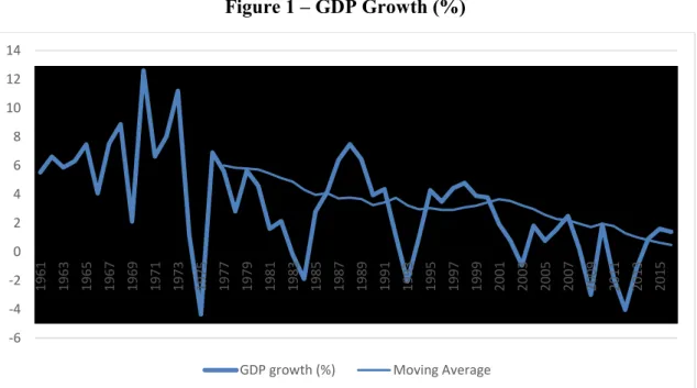
We start by analyzing economic growth, described in Figure 1. From 1960 until 1973, we have a period of high growth and convergence towards industrialized countries, which was mainly due to the shift of resources from the agricultural sector to the industrial sector that occurred with the industrialization process. Between 1974 and 1985, we have a period of accentuated decline of economic growth, mainly due to the political and economic instability that came with the revolution in 1974. After two IMF interventions in 1978-79 and 1983-85, and joining the EEC (European Economic Community) in 1986, there is an inversion of this tendency and an increase in economic growth from 1986 to 1998. However, from 1999 onward, there is a decrease of growth and a propensity for stagnation.

According to Andrade, Duarte & Simões (2012), the growth in the 1986-1998 periods is explained by “…implementation of better macroeconomic policies (associated with the process of nominal convergence on the way to the euro in 1990s), structural reforms, especially in the financial, labour and product markets, but also investments in physical and human capital, and technology enhancing factors”; while the growth in the years from 1999 onward is explained by the low levels of educational attainment, technological infrastructures and investment in R&D, as well as macroeconomic instability generated by an increase in the size of government and in the specialization in low productivity services.

When it comes to public spending, Tanzi and Schuknecht (2000) show that the vast majority of industrialized countries significantly increased their public spending, as well as their tax levels, in the post-World War II period, especially between 1960 and 1980. This conduct is explained by the growing influence of Keynesianism, with the development of the

(10)

Figure 1 – GDP Growth (%)

Source: World Bank, “World Development Indicators”

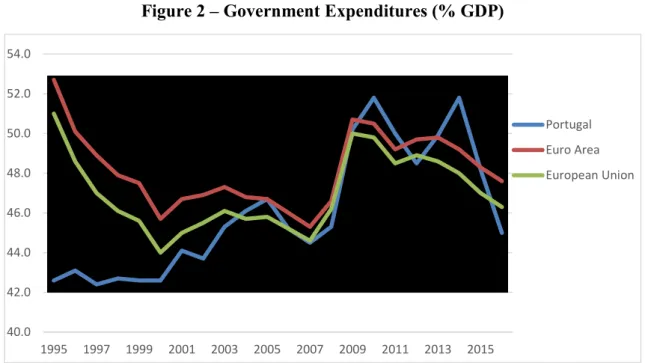
concept of externalities and the theory of public goods; the popularity of socialism and its redistributive policies; the stabilization tools that can be provided, for example, to reduce business cycles and unemployment; and the protection it provides to its citizens in risky situations, like temporary unemployment. Cunha, J. e Braz, C. (2012) explain that these policies were sustained by a high economic growth and a very favorable demographic structure (which resulted from the Baby Boom), with a high proportion of people of working age and, therefore, potential net contributors. The authors defend that most countries did not take into account that the revenues and expenditures should be adjusted to the resources generated by the economy to ensure the sustainability of public finances. Through the analysis of public expenditure (in % GDP), described in Figure 2, we can see that, in the period of 1995 to 2010, Portugal followed the trend of increase in public spending (even though with a considerable lag,), converging to the average of the euro area and the European Union. The large increase in 2009 is in response to the international crisis by most member states of the union, whether through automatic stabilizers, or through stabilization policies. Nevertheless, as revenues were insufficient, Portugal accumulated fiscal deficits that resulted in a growing public indebtedness. In the last two decades, the fiscal deficit never fell significantly below 3% of GDP (see Figure 3), which, combined with small economic growth, resulted in a gradual but sustained rise in public debt since 2000 (see Figure 4). In 2009, the “debt increase” shifted to a much steeper path, reaching 130% of GDP in 2014.

-6 -4 -2 0 2 4 6 8 10 12 14 1961 1963 1965 1967 1969 1971 1973 1975 1977 1979 1981 1983 1985 1987 1989 1991 1993 1995 1997 1999 2001 2003 2005 2007 2009 2011 2013 2015

(11)

Figure 2 – Government Expenditures (% GDP)

Source: Eurostat, “General Government Expenditure and main aggregates”

Figure 3 – Fiscal Indicators (% of GDP)

_{Source: OECD Economic Surveys, Portugal 2012}

40.0 42.0 44.0 46.0 48.0 50.0 52.0 54.0 1995 1997 1999 2001 2003 2005 2007 2009 2011 2013 2015 Portugal Euro Area European Union

(12)

Source: OECD Economic Surveys, Portugal 2017

In the period of 1995-2010, as a result of the introduction of the euro and the transition to monetary stability, nominal and real interest rates in Portugal fell drastically. As described by Guillemette and Turner (2013), foreign investors “… rushed to invest in peripheral euro area countries, assuming that not only exchange rate risks, but also sovereign default risks, had largely been eliminated by the currency block”. The consequence of these large capital inflows were large current account deficits, as described in Figure 5. As a result, the net international investment position has deteriorated substantially (more specifically, from -9,3% in 1996 to -118,7% of GDP in 2013, as described in Figure 6). The international crisis caused risk perceptions to be re-adjusted, resulting in a decrease of capital inflows for the peripheral countries, and a lower sustainability of the deficits of current accounts as well.

The combination of a rising public and external debt, slowing economic growth and the instability that came with the international financial crisis, led to a loss of confidence that Portugal would be able to fulfill its financial obligations, reflected in the lack of access to long-term financing at sustainable rates, culminating in the necessity of a financial assistance program signed with the European Union and the International Monetary Fund (EU-IMF). The outcomes seem to be in line with the goals of the program. Economic growth is picking up, government expenditure are decreasing (as we can see in Figure 2), public deficit is decreasing, public debt is beginning to get under control, and predicted to decrease (as we can see in Figure 4), and its outlook is now seen as acceptable by 3 out of the 4 main rating agencies. However, a closer analysis of Figure 4 shows the fragility of the current situation.

50 60 70 80 90 100 110 120 130 140 150 2000 2005 2010 2015 2020 2025 2030

Under current plans Higher interest rate Lower inflation

(13)

Figure 5 – Current Account to GDP in Portugal (%)

Source: OECD, “Current Account Balance”

Figure 6 – Portugal's Net International Investment Position (% of GDP)

Source: Eurostat, “Net international investment position in % of GDP”

An increase in the interest rates or the inflation rates can lead the path of public debt back to unsustainability.

The last topic we will address in this section is population ageing, the changes in the demographic structure, and the consequences for fiscal policy. Even though Portugal (and other EU member states) are familiar with this concept, its consequences have to be taken into account for policies that will affect future generations. Many policies of the welfare state that

-16 -14 -12 -10 -8 -6 -4 -2 0 2 4 1996 1997 1998 1999 2000 2001 2002 2003 2004 2005 2006 2007 2008 2009 2010 2011 2012 2013 2014 2015 2016 Portugal EU28 -140 -120 -100 -80 -60 -40 -20 0 1996 1998 2000 2002 2004 2006 2008 2010 2012 2014 2016 NII (% of GDP)

(14)

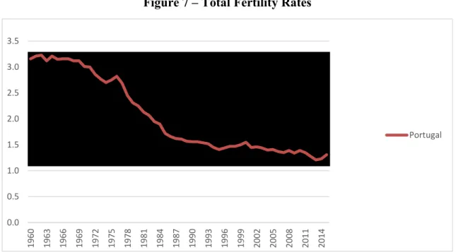
provide citizens protection against risk (like social security), were institutionalized in a much more thriving demographic environment, with a younger population and with optimistic expectations of economic growth. The main reasons for this development are the continuous fall in fertility rates, combined with the increase in life expectancy, as shown in Figure 7 and Table 1, respectively.

The change in fertility rates is due to a number of factors that can be attributed either to a cultural shift or to the economic situation. As we can see in Figure 7, after the euphoria of the post-war and the baby boom exhausted, the fertility rates fall steadily, down below the theoretical level of substitution of generations of two children. Inevitably, populations will decrease in the long-run in European countries and the demographic structure of the population will change, with a higher proportion of elderly in total population, if there are not enough migration gains to counterbalance this phenomenon.

The increasing life expectancy of individuals relates to economic activity in a progressively problematic way, where the benefits of the elderly are inversely adjusted to the development of life expectancy. In these circumstances, old age ceases to be a singular risk that social security prevented in the few terminal years of every pensioner, substituting the earnings when the individual leaves the labor market definitely, and creating a new risk. This additional risk is associated with the possibility of pension benefits being insufficient to guarantee a decent standard of living to the beneficiary that faces new threats associated with longevity (mainly regarding healthcare and the funding of those pensions). The risks associated with dependency and with prolonged illness have a very significant effect in Portugal, as well as in other developed countries. Until now, the socialization of these risks associated with longevity has been low. The family solution has prevailed so far and the institutionalization of the elderly in residential nursing homes works as a solution of last resort, when the situations become too complicated to be managed inside the family. However, the shift in family structures in the last decades has increased the number of people with no family support to help them against these risks, which will lead to a higher demand of public long-term care services. The need of public protection against longevity risks is likely to increase even more in the future, given the information provided in Table 1.

(15)

Figure 7 – Total Fertility Rates

Source: Eurostat, “Fertility rates”

Table 1 – Life Expectancy

2005 2006 2007 2008 2009 2010 2011 2012 2013 2014 2015

Life expectancy at birth (females) 81,3 82,3 82,2 82,4 82,6 82,8 83,8 83,6 84 84,4 84,3

Life expectancy at birth (males) 74,9 75,5 75,9 76,2 76,5 76,7 77,3 77,3 77,6 78 78,1

Healthy life years at birth (female) 57,1 57,9 57,8 57,6 56,4 56,6 58,6 62,6 62,2 55,4 55

Healthy life years at birth (male) 58,6 60 58,5 59,1 58,3 59,3 60,7 64,5 63,9 58,3 58,2

Source: Eurostat, “Healthy life year indicators”

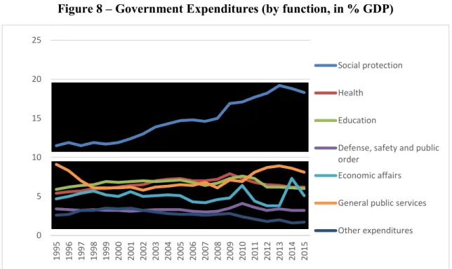
We also need to take into account the pressure of ageing on government budgets and future generations. The evidence presented in Figure 8 and Table 2, regarding the development of public expenditures by function and old age dependency ratios, respectively, reflects the increase of government expenditures associated with the ageing phenomenon, as well as the burden that is going to fall on the working age population, or to be covered by future generations. Even though the costs regarding healthcare have been kept under control, as we can see from Figure 8, it seems obvious that social protection is the account that is putting pressure on public finances, and that this behavior is, mainly, due to old age related expenditures. While almost all accounts are below the 10% of GDP line, government expenditures with social protection were always above 10%, steadily increasing and diverging from all the other accounts, with 18,8% in 2012. Table 2 provides how old age dependency ratios changed overtime, as well as how they are predicted to change in the future, and are a good indicator of the burden that will fall upon current middle-aged/active and future generations. 0.0 0.5 1.0 1.5 2.0 2.5 3.0 3.5 1960 1963 1966 1969 1972 1975 1978 1981 1984 1987 1990 1993 1996 1999 2002 2005 2008 2011 2014 Portugal

(16)

Figure 8 – Government Expenditures (by function, in % GDP)

Source: Eurostat, “Government Expenditures by function”

Table 2 – Old Age Dependency Ratios

Actual Projected 1965 12,8 1996 22,2 2003 24,9 2010 27,5 2020 34,6 1970 14,9 1997 22,6 2004 25,3 2011 28,2 2030 43,6 1975 15,7 1998 23,0 2005 25,7 2012 28,8 2040 55,6 1980 17,8 1999 23,4 2006 26,0 2013 29,4 2050 65,3 1985 18,2 2000 23,7 2007 26,3 2014 30,3 2060 64,9 1990 20,0 2001 24,2 2008 26,6 2015 31,1 2070 67,0 1995 22,0 2002 24,6 2009 27,0 2016 31,8 2080 69,0

Source: Eurostat, “Old Age dependency ratios”

This indicator reflects the number of elderly people (with 65 years or more) per 100 active/working age people (with age between 15 and 64). Therefore, a higher dependency ratio implies a higher “burden” on the working population with the expenditures of their elderly. As we can see, the projected ratios for the future are quite alarming, with more than 1 elderly per 2 people of working age. And the scenario may be even worse, if we take into account that some of the people between 15 and 64 years may be studying, unemployed or non-participating in the labor force. Also, even though life expectancy at birth has increased, there is not only, a huge difference when compared to the healthy life years at birth indicator, but also a difference in the increase in years between the two indicators, with healthy life years increasing at a lower rate than life expectancy.

0 5 10 15 20 25 1995 1996 1997 1998 1999 2000 2001 2002 2003 2004 2005 2006 2007 2008 2009 2010 2011 2012 2013 2014 2015 Social protection Health Education

Defense, safety and public order

Economic affairs General public services Other expenditures

(17)

Summing up, with an ageing population and the number of beneficiaries of public budgets growing more than contributors, the distributive needs will keep increasing, which will put more pressure on national budgets. However, Portugal’s public finances are already under pressure, and even though the overall economic and financial outlook is improving, public debt is still far from assured sustainability.

3. Deficit and Debt as a not well-defined measure

In general, policy and decision makers take deficit and debt as the main guiding tools in fiscal policy. Take, for example, the target defined for public deficits at 3% or less of GDP for the countries in the European monetary Union. The main concerns with the traditional fiscal measures, specifically, debt and deficit accounting, are their arbitrary nature, and their focus on the current and short run effects of fiscal policies.

Government expenditures and revenues, as well as the level of public debt, are published in annual government budgets and, therefore, capture the short-run effects of fiscal policy. This implies that a change of policy in a given year that yields an impact throughout many years in the future (or for more than one year, at least), may bear the risk of only being associated with its short-run effects (given by the budget of that same year), while its effects for the other years are going to be incorporated in those yearly budgets and may be disassociated with that specific policy. If agents are rational and forward looking, they will consider the impacts of fiscal policy on their lifetime budget constraint, and will readjust their consumption and savings level according to the new policy. It is very unlikely that an annual government budget will be able to capture the whole effect of these changes, especially if they affect generations born in the future. Therefore, it is important to measure the effects of fiscal policy in the long-run, as it may affect the life cycle resources of current and future generations, by redistributing resources among them.

As established in Auerbach, Kottlikoff and Leibfritz (1999), the arbitrary nature of these measures relies on the fact that they depend on how different governments or different countries choose to define their expenditures and their revenues. Governments can conduct any sustainable fiscal policy, and at the same time choose its accounting so as to report any surplus or deficit that they want. They are able to enact policies with huge intergenerational redistributive fiscal effects while reporting a “balanced budget”; or enact apparently identical fiscal policies with dramatically different time paths of reported deficits. However, the way

(18)

governments choose to define their revenues and expenditures should be irrelevant for actual fiscal policy, since the economic effects of the fiscal policy followed will not depend in any way on the accounting labels chosen.

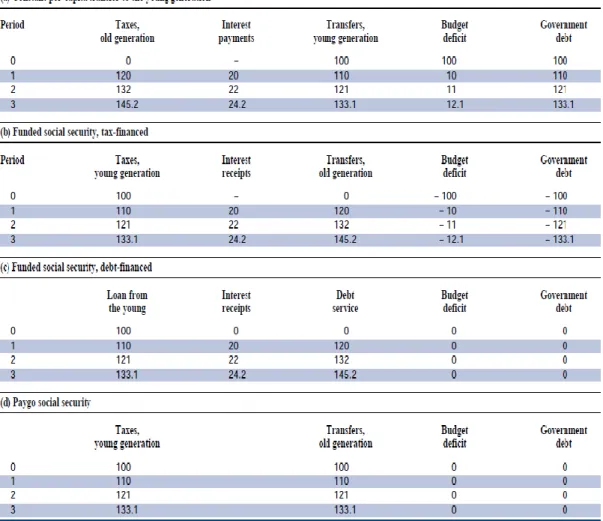
We demonstrate these concerns with an example described in Raffelhüschen and Walliser (1999). In this example, we consider a model of two generations (young and old), that only live for two periods, and where there is no government activity before period 0. It is also assumed that the interest rate is 20% and that population growth is 10%. Given this model, we now study the impact of four different intergenerational redistribution policies on government budgets, with the results described in Table 3, also taken from Raffelhüschen and Walliser (1999).

Table 3 – Traditional Fiscal measures

(19)

In scenario (a), there is a transfer of 100 units granted to the young generation in the first period, which is only paid for by that same generation in the next period. So, in period 0, there is an expenditure of 100 units that is not paid and, as a result, the budget deficit and government debt are also of 100 units in this period. In the next period (period 1), the now old generation has to cover the transfer that it has received in the previous period, so it pays taxes of 120 units, which is equal to the 100 units of transfer received in period 0, plus 20 units of interest payments on the public debt. If the policy is maintained in period 1, the young generation from period 1 receives 110 units, which increase from 100 units in period 0 due to population growth of 10%. In period 1, the government collects taxes of 120 units, and has expenditures with, not only of 110 units in transfers, but also of 20 units in interest payments, amounting to a total of 130 units. Thus, the deficit in period 1 will be of 10 units, and the government debt will accumulate to 110 units. If this policy is maintained for future periods, we can see that both government deficit and debt will grow at the same rate as the population. In scenario (b), the policy is the institution of a tax-financed pension system, in which generations will discount for their own pensions through the payment of taxes when they are young, and receive the pension benefits in the following period, when they are old. If this policy starts in period 0, the government will report a surplus and net wealth of 100 units, since young generations of this period will be taxed in 100 units, and old generations of this period will not receive any amount, since they have not discounted in the previous period. In period 1, the government has to pay 120 units to the old generation (100 units taxed in the previous period plus interest), and amounts revenues of 20 units, from the interest on accumulated wealth in the previous period, plus 110 units in taxes from the young generations, which increased from 100 units in the previous period due to the population growth. Therefore, the surplus in period 1 is of 10 units and net wealth is of 110 units, and both these accounts will grow at the rate of the population if the policy is maintained.

We now turn to scenario (c), which is identical to scenario (b), but with one difference: the payments made by the young generations are classified as loans, which the government invests on the capital market. This implies that the amount collected from the young generations in each period does not classify as government revenue, and it will report a balanced budget and no debt in period 0. In period 1, if we assume perfect capital markets, the amount invested in period 0 (100 units) will yield a return of 20%, which is the defined interest rate. The interest receipts plus the amount invested will be enough to cover the debt to the now old generation of period 1 (loan granted plus interests). If this policy is maintained,

(20)

both the loans from the young generation, and the respective debt payments in the following periods grow at the same rate as the population. However, in this case, government has a balanced budget in every period and, hence, has no debt.

The last scenario (d) describes a policy that introduces a pay-as-you-go pension system. Under this type of system, the transfers received by the old generation in each period will equal the tax payments of the young generation of the same period. Basically, young generations finance the transfers of the old generations of their own period, expecting that the young generations in the next period will do the same for them. In this case, both the taxes paid by young generations and the transfers received by the old generations will grow at the same rate as the population. Also, taxes paid and transfers received are the same in each period, the budget is always balanced and the government debt is always equal to zero.

If we analyze all four policies using the traditional fiscal measures (deficit and debt accounting), we conclude that: the policy enacted in scenario (b) achieves the most satisfying results, increasing the amount of net wealth over the years; the policy enacted in scenario (a) achieves the least satisfying results, increasing the amount of government debt over the years; policies (c) and (d) have no effect on the public budget and debt level, and are equivalent to one another.

However, if we analyze these policies in terms of intergenerational distribution, and in terms of changes in the lifetime budget constraint, we conclude that, not only are the first three policies identical, but also indifferent, since they do not present any changes in terms of the present value of the net tax payments for each generation. In each one of these policies, whether the generations are receiving first and paying in the following period, or paying first and receiving in the following period, these payments and transfers take into account the opportunity cost of money, given in this example by the interest rate of 20%. In other words, the net present value of taxes paid minus transfers received over the life cycle for each generation has not changed. For that reason, rational agents do not have any incentive or reason to change their behavior with the policies described in scenarios (a), (b) or (c). We also conclude that the policies described in scenarios (d) and (c) are not equivalent. In scenario (d), the introduction of the pay-as-you-go system automatically increases the consumption possibilities of the old generation in period 0 who did not contributed to the system. This increase is financed by all other subsequent generations, who have their consumption possibilities reduced, since their rate of return under the pay-as-you-go system is equal to the population growth, which is lower than the interest rate.

(21)

4. Generational Accounting

Auerbach, Kottlikoff and Leibfritz (1999) state that fiscal policies have real effects, because they “…(1) alter economic incentives, (2) redistribute from different generations to the government, (3) redistribute within generations, or (4) redistribute across generations”, and they provide an alternative methodology to study these effects, called generational accounting, which is based on the intertemporal budget constraint of the government, described in equation (1). This equation establishes that the present value of the net tax payments (which encompass taxes and contributions paid less social security, welfare, and other transfer payments received) of current and future generations have to be enough to cover the present value of government expenditures and the current level of net public debt. In short, it requires either current or future generations to cover overall public spending. Since one of the goals is to assess how the “fiscal burden” is distributed among different generations, the net tax payments of current and future generations must be analyzed separately. ∑ 𝑁𝑡,𝑘+ (1 + 𝑟)−(𝑘−𝑡) ∑ 𝑁𝑡,𝑘 ∞ 𝑘=𝑡+1 = ∑ 𝐺𝑠 ∞ 𝑠=𝑡 (1 + 𝑟)−(𝑠−𝑡)_{− 𝑊} 𝑡𝑔 (1) 𝑡 𝑘=𝑡−𝐷

As can be seen in equation (1), there are 4 main variables. Starting from left to right, the first element consists of the sum of the generational accounts of current generations. The term 𝑁_𝑡,𝑘 represents the net tax payments of the generation born in year k, discounted to year t (the base year), and k goes from t – D (where D stands for the maximum age, in the base year) to t (the generation born in the base year). The second element of equation (1) represents the present value of the sum of the generational accounts of future generations. It is important to point out that these two variables encompass all the public revenues and expenditures that are directly dependent on the age structure of the population, and whose payments or benefits can be directly attributed to the population according to their age. Therefore, the third element of equation (1) consists of the present value of the sum of the net public expenditures (expenditures minus revenues) that do not depend on the age structure of the population. This includes government’s purchases of goods and services whose benefits are difficult to attribute to specific generations. This implies two things: 1 – generational accounting only tells us which generations will have to pay for the net public expenses defined by G, but it

(22)

does not tell us which generation benefits from them, or how valuable or beneficial they are; 2 – generational accounting is not able to completely show the full net benefit or burden for each generation from fiscal policy as a whole, but it is able to show the full net benefit or burden for a generation if there are changes from fiscal policy affecting variables included in the net tax payments (taxes and transfers), from all levels of government (federal, state, and local).The last element of equation (1), 𝑊_𝑡𝑔, encompasses the government’s net wealth in year t (basically, the public assets minus public debt). Finally, looking at equation (1) overall, we can identify a “zero sum” characteristic for this intergenerational budget constraint. That implies that, for example, given a certain level of government net wealth, an increase in the present value of net public expenditures (third element of equation (1)) requires an increase in the present value of the generational accounts of either the current or future generations, or a combination of both (first and second element of equation (1)).

We now proceed to a more detailed analysis on how to estimate the generational accounts, which follows a two-step process: 1 - Projecting the average taxes and transfer payments of each living generation for each year in the future during which at least some members of the current generation will be alive; 2 – Taking the projections estimated in the first step and discounting them to the base year, and also taking into account the probability of the people from each generation to be alive in the future years. Thus, the generational account N_t,k is given by equation (2):

𝑁_𝑡,𝑘= ∑ 𝑇_𝑠,𝑘 𝑘+𝐷 𝑠=𝜆 𝑃_𝑠,𝑘(1 + 𝑟)−(𝑠−𝜆)₍₂₎ T_s,k= ∑ ℎ_{𝑠,𝑘,𝑖} 𝑖 (3)

Where 𝜆 = 𝑚á𝑥(𝑡, 𝑘). The 𝑇𝑠,𝑘 variable stands for the net tax payments that are

expected to be paid in year s by an average person of the generation born in year k. This can be better described by equation (3), where ℎ𝑠,𝑘,𝑖 stands for the average tax (if h > 0) or

average transfer (if h < 0) of type i paid or received, respectively, in year s by an average person born in year k. The term Ps,k stands for the expected number of people who were born

(23)

in year k and are still alive in year s. Notice that equation (2) is defined for the members of the current generation that were born before or after the base year, but we only take into account the net tax payments after the base year, discounted according to the year which they were made, on a present value base analysis. For the people born before year t, the sum begins in year t and is discounted to year t (this analysis is forward looking, so we don’t take into account the net taxes already paid prior to the base year). For the people born in year k > t, the sum begins in year k and is discounted to that same year k. The net tax payments of the people born after year t will also have to be discounted to year t, as it can be seen in equation (1).

One of the crucial assumptions in generational accounting is that the behavior of economic agents will not change, and that fiscal policy is stable. In other words, generational accounting provides us with some insights regarding the “fiscal burdens” that fall upon current and future generations, if the current fiscal policy is maintained. With this assumption, it is possible to calculate the age profile of the expected average taxes paid and transfers received per capita for the future, starting from the age profile of payments of the base year:

ℎ_{𝑠,𝑘,𝑖} = ℎ_{𝑡,𝑡−(𝑠−𝑘),𝑖}(1 + g)(s−t)₍₄₎

Basically, equation (4) states that the taxes paid and transfers received of a person in year s (given s > k), with an age of s – k, will be the same as those observed for people of the same age in year t, and adjusted for the gains in productivity between year s and the base year. These gains in productivity are given by the annual growth rate of productivity (g), which we will assume to be constant.

For the future values of net public expenditures, we will also assume that they evolve at the same rate as taxes and transfers included in the net tax payments, that is, G grows at the rate of productivity, given by g, for future years.

Since we know the government’s net wealth 𝑊_𝑡𝑔 , and we can determine the sum of the generational accounts of current generations and the present value of the sum of net public expenses, we can use them to determine the sum of the generational accounts of future generations, as a residual. More specifically:

(24)

(1 + 𝑟)−(𝑘−𝑡) _{∑ 𝑁} 𝑡,𝑘 ∞ 𝑘=𝑡+1 = ∑ 𝐺_𝑠 ∞ 𝑠=𝑡 (1 + 𝑟)−(𝑠−𝑡)_{− 𝑊} 𝑡𝑔− ∑ 𝑁𝑡,𝑘 (5) 𝑡 𝑘=𝑡−𝐷

Thus, the “fiscal burden” that will fall upon future generations is the part of the sum of present value of the net public expenditures that are not covered by government net wealth and by the net tax payments of current generations. With this information, even though we are not able to explain exactly how this “fiscal burden” that is left to the future generations is going to be distributed among them, if we assume that the average net tax payments per capita of the future generations increases by a fixed growth rate of productivity, we can actually estimate the average per capita present value lifetime net tax payments for the people of each future generation (making lifetime net tax payments a fixed share of lifetime income). Hence, we define the generational account of a representative agent born in year k and still living at time t in the following equation:

𝐺𝐴_𝑡,𝑘𝐶𝑈𝑅𝑅= ∑ Ti,k k+D

i=t

Pi,k(1 + r)−(i−t)⁄𝑃𝑡,𝑘 (6)

If we use the definition established in equation (2), we can rewrite equation (6) as:

𝐺𝐴_𝑡,𝑘𝐶𝑈𝑅𝑅 ₌𝑁𝑡,𝑘

𝑃_𝑡,𝑘 (7)

Finally, we need to determine the generational accounts of future generations, which is given in equation (8). 𝐺𝐴_𝑡+1𝑓 = ∑ 𝐺𝑠 ∞ 𝑠=𝑡 (1 + 𝑟)−(𝑠−𝑡)− 𝑊𝑡𝑔− ∑𝑡𝑘=𝑡−𝐷𝐺𝐴𝑡,𝑘𝐶𝑈𝑅𝑅𝑃𝑡,𝑡−𝑘 ∑∞ 𝑃_𝑘,0 𝑘=𝑡+1 (1 + 𝑔_{1 + 𝑟)} 𝑘−𝑡−1 (8)

This equation (which is a rewrite of equation (5)) gives us the part of net government expenses that is not financed by current generations, which is then allocated equally to be covered by future generations.

(25)

But we need to take into account that the expected remaining years of life of people who are still alive, at year t (given by k + D – t), is different according to the year that each person was born. Therefore, the per capita generational accounts are not directly comparable among themselves. However, we can compare the per capita generational accounts of the people born in the base year, and the people of the future generation, since both take into account the net tax payments over their entire lifetimes and are discounted back to the base year. We can also use a relative approach, given by:

𝜋 =

𝐺𝐴𝑓𝑡+1

𝐺𝐴_𝑡𝐶𝑈𝑅𝑅

∗ (

1+𝑟

1+𝑔

)

(9)

5. Data Analysis and Assumptions

The empirical evaluation of the intertemporal budget constraint requires: projections of population, taxes, transfers, and government expenditures; an initial value of government wealth; a growth rate and a discount rate. We consider the impact of total, not just national, government. We establish 2010 as the base year, and consider a 100 years range of analysis, that is, from 2010 to 2110.

5.1. Population

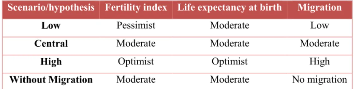
Since generational accounts are defined as per capita net taxes in present terms, the values are influenced by the size and age of the population in each generation. The size of the population is relevant in order to distribute the amount of net taxes needed to cover government expenditures and to service the debt. Since the size of future generations is expected to decrease in the coming years, the total amount of net taxes are going to be divided by a smaller number of people. In addition, the structure of the population critically influences the absolute amount of net taxes, since most taxes paid and transfers received are age-specific or highly related to the person’s age. The projections used to compute the generational accounts are based on the 2009 population projection estimates by age and gender provided INE (Instituto Nacional de Estatística) from 2010, which is the base year, until 2060. These estimates provide four different scenarios (central, low, high and without migration), which are described in Table 4.

(26)

Table 4 – Population Projections in Portugal, by Scenario

Scenario/hypothesis Fertility index Life expectancy at birth Migration

Low Pessimist Moderate Low

Central Moderate Moderate Moderate

High Optimist Optimist High

Without Migration Moderate Moderate No migration

Source: INE, “Projecções de População Residente em Portugal”, 2009

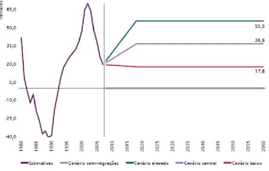
For each of these scenarios, the initial values (of 2008) are identical, but they incorporate different hypothesis regarding future values of fertility, mortality and migration rates. Regarding the projections for net migration, they are always positive. They display a linear trend (significantly increasing for the high and central hypothesis, and slightly decreasing for the low hypothesis) from 2007 until 2018, and they remain constant for the rest of the period in analysis, as it can be seen in Figure 9. Since we consider these migration scenarios questionable (and the hypothesis for the other two variables are “moderate”), we decided to use the scenario without migration for population projections by age and gender from 2010 until 2060. Given that we are aiming for a 100 year period analysis, we made our own calculations to extend the population projections to 2110. For that, we needed to estimate the number of people who would be born each year, as well as the number of people who would die each year, for each age group, from 2061 to 2110. Given the complexity of the model used for the projections in the previous periods (Poisson-Lee-Carter models), we opted for a different approach, for simplicity. We started by calculating age specific death rates (ASDR) for the 2010-2060 period, by year, gender and age. Then, we used these rates to estimate a trend function for each age group, and used this function to estimate the age specific death rates from 2061 until 2110. Finally, we only need to estimate the number of people who would be born each year. Instead of birth rates, we estimated number of births, since this function is more monotonic. Also, we have used only the last 10 years of the sample (2050-2060) to estimate the trend function, given the function shows a stabilization on the last years, and these results fit better the data and the other projections.

(27)

Figure 9 – Migration levels for the different scenarios

Source: INE, “Projecções de População Residente em Portugal”, 2009

5.2. Fiscal data

The information regarding government revenues and expenditures was retrieved from the DGO (Direção-Geral do Orçamento), more specifically, from the consolidated general government accounts (public account basis) presented in the CGE reports (Conta Geral do Estado) for the years available (2010 to 2015). For the years after these reports, as mentioned before, it is assumed that government’s revenues and expenditures that do not depend on demographics (the ones included in variable G) evolve at the rate of productivity, given by g. In other cases, we break the purchases down into age-specific components (e.g.: Expenditures with current transfers, mostly consisting of pension benefits) and assume that each component remains constant per member of the relevant population, adjusted for the overall growth in productivity g. This causes different components of government purchases to grow more or less rapidly than productivity, according to whether the relevant population grows or shrinks as a share of the overall population.

(28)

In our calculations, we consider government spending (that we describe as G) as the sum of government consumption, subsidies and net investment (considered as capital expenditures minus capital revenues).

The other components, consisting of direct taxes, social security contributions, indirect taxes, and current transfers (consisting mainly of social security expenditures) are highly dependent on population structure, and need to be assigned accordingly. Essentially, for the years for which government values and forecasts are available, these aggregate amounts are distributed by age, based on cross-sectional relative age-tax and age-transfer micro-profiles derived from cross-sectional microdata sets. For years beyond those for which government values and forecasts are available, age-specific average tax and transfer amounts are assumed to equal those for the latest year for which forecasts are available, with an adjustment for productivity growth.

Finally, since we are considering a finite period of 100 years, we will not assume that the government’s net debt has to be fully paid by current or future generations until the last period considered in the analysis. Instead, we will consider that the generations will have to “service” de debt, and assume that it grows less quickly than the rate of discount, as to not become explosive. Therefore, in our calculations, we have assumed that the variable W_tg is equal to zero, and the interest payments on public debt were included in the variable 𝐺_𝑠, hence, growing at the same rate.

5.3. Micro-profiles

The general rule regarding tax incidence is to assume that taxes are paid by according to the base on which they fall upon: income taxes on income, consumption taxes on consumers, and so forth. In small open economies (like Portugal), there is a need to modify generational accounting by allocating changes in corporate capital income taxes to generations in proportion to their labor income. The reason is that an increase in the corporate income tax rate in a small open economy will produce an immediate capital outflow, thereby lowering the marginal product of labor and the wage; i.e., the corporate tax will be immediately shifted to workers. As we established in the previous section, the categories of taxes and transfers are set according to the consolidated general government accounts (public account basis) presented in the CGE of each year that are available. The taxes and transfers are then allocated according to income, transfer and consumption micro-profiles, estimated from the survey Inquérito às Despesas das Famílias from 2010/2011. Direct taxes were

(29)

distributed based on a wage earnings profile (which is grossed up to include property income and self-employment earnings), as well as corporate income taxes. Since social security contributions are imposed as employment taxes, they were also distributed according to the wage profile. Indirect taxes (which mainly consist of taxes on consumption) were distributed according to a consumption expenditures profile. Expenditures with current transfers (consisting of social security and other transfers), were distributed according to a general transfers receipt (which consist of pensions and other transfers). As a general rule, the profiles obtained from the microdata are assumed to stay constant over the entire projection period. This procedure maintains base-year economic structures indefinitely.

5.4. Growth and Discount rates

It is necessary to specify an appropriate annual rate of productivity growth, since it will influence the projections of future values of age-specific tax payments and transfers, and an appropriate interest rate, in order to discount all future payments and be able to express them in present value terms of the base year. Despite there being a lot of uncertainty surrounding the definition of both the discount rate and the future productivity growth rate, the appropriate interest rate is mainly influenced by the risk regarding public revenues and expenditures, while the appropriate growth rate is mainly influenced by the EU average and the country’s own economic outlook in the future. Starting with the discount rate, usually, government revenues and expenditures have more risk than non-risky long-term government bonds, but they are not as risky as the return on risky assets. However, we also have to take into account that this risk may be different for each country, depending on the outlook of sustainability of public finances. In the case of Portugal, the country’s inability to finance itself at sustainable interest rates led to the need of a financial assistance program signed in 2011, and even though it is now able to finance itself at reasonable interest rates, the large deviations in the interest rate over the last decade generate uncertainty regarding the country’s capacity to keep financing itself at the current rates in the long run. This also had an impact on the prospects of the future productivity growth rate, given that the corrective measures applied during these years to reduce government deficits and stabilize public debt had a negative impact on economic growth, and since these corrective policies have to be maintained for future years in order to generate public surpluses and decrease public debt, there is a lot of uncertainty regarding future economic growth rates. Given the sensitivity of generational accounts with respect to the values of these rates, and, as we pointed above, the uncertainty surrounding the definition of appropriate discount and productivity rates, it remains a standard practice to

(30)

estimate generational accounts for a range of discount rates and productivity growth rates. Hence, we define three interest rates and three productivity growth rates, based on Portugal’s own expected interest and growth rates for different possible scenarios, provided in Table 5. We have also established an additional scenario, in which the variable 𝐺_𝑠 grows at a rate of 0,8%. The results from these scenarios will be further discussed in section 7.

Table 5 – List of productivity growth rates (g) and discount rates (r)

g = 1% g = 1,5% g = 2%

r = 3% r = 5% r = 7% r = 3% r = 5% r = 7% r = 3% r = 5% r = 7%

6. Results and Comparisons

In this section, we start by making a brief analysis of the net tax payments in 2010, by age. As we can see in Figure 10, the set of accounts exhibits a concave pattern with respect to age. When people are young, they receive transfers (e.g., child benefits or educational allowances) and pay consumption taxes. During their working lives, they continue to pay consumption taxes but also pay taxes on their labor and capital income in the form of personal income taxes and payroll taxes, so we can see that their net tax payments increase. When workers reach older ages, they start receiving transfer receipts (e.g., pensions), and so the net tax payments start to decline. From 60 onwards, we can see that transfer payments received generally start to exceed the tax payments so that net tax payments become negative, that is, they become net transfers. We can also see that the absolute amount of net transfers’ declines from 75 onwards, due to a decrease in the population levels. However, one would expect the net tax payments to be negative for younger generations. This has to do with the distribution of indirect taxes by age, which are allocated according to a micro-profile of consumption expenditures. Since the data provided the expenditures by households, and we needed to allocate them to individuals, we resorted to an equivalence scale defined as “OECD-modified scale”, which assigns a value of 1 to the household head, of 0,5 to each additional adult member, and of 0,3 to each child. And given our results, even in the case when education expenditures are allocated as transfers, the consumption taxes outweigh them, resulting in positive net tax payments.

(31)

Figure 10 – Portugal's Net Tax Payments in 2010, in millions of dollars, by age

Source: Own calculations

Now, we follow with an analysis of the generational accounts in 2010 (see Figure 11 and Table 6), and compare with the generational accounts in 1995 (see Figure 12 and Table 7)1. We can see that the accounts are positive and increase initially with age. The present

value of a generation’s remaining lifetime net tax payments is generally highest for generations at the beginning or at the middle of their work spans, as it does not include child and educational benefits received in youth, more and more people start to enter into the workforce, and they progress in their working career, earning higher levels of income and, therefore, paying more taxes. Then, they begin to decline for older generations, since part of their net tax payments were prior to the base year. The generations that become net transfers start at 47, and then it starts increasing again, since part of the transfer payments were prior to the base year.

When workers reach older ages, the sum of future net tax payments tends to decline as future transfer receipts (e.g., pensions) gain in importance compared with future tax

1 In this base case, we are not treating public expenditures on education as transfer payments, and therefore, not

allocating them by age, hence their value in the Table being zero (that scenario is described in Table 13). Instead, they are treated as government purchases and are added to the variable 𝐺, as done in Auerbach, Kottlikoff and

Leibfritz (1999). -1500 -1000 -500 0 500 1000 1500 2000 0 3 6 9 ₁₂ ₁₅ ₁₈ ₂₁ ₂₄ ₂₇ ₃₀ ₃₃ ₃₆ ₃₉ ₄₂ ₄₅ ₄₈ ₅₁ ₅₄ ₅₇ ₆₀ ₆₃ ₆₆ ₆₉ ₇₂ ₇₅ ₇₈ ₈₁ ₈₄ ₈₇ ₉₀ ₉₃ ₉₆ ₉₉

(32)

payments. We can also see that the absolute amount of net transfers’ declines from 65 onwards, due to a decrease in the population remaining lifetime.

If we compare our results with the generational accounts of Portugal in 1995, provided in Auerbach, Kottlikoff and Leibfritz (1999), we can see that the accounts follow a very similar pattern, with respect to age. However, we can see that the generational accounts hit lower values after 50 years. Comparing Figures 11 and 122, in 1995, the lowest level is

between 50.000 and 100.000 dollars, while in 2010, it’s close to 150.000 dollars. We can also see that the “fiscal burden” that will fall upon future generations increased significantly. In 1995, representative member of future generations would have to pay 48,7% (or 1,5 times) more taxes than a representative member of the current generation. In 2010, that value increased to an alarming 372,4% (or to 4,9).

2 The values in Figure 12 correspond to the values in Table 7, updated according to the GDP deflator

(33)

Figure 11 – Generational Accounts 2010 (thousands of dollars)

Figure 12 - Generational accounts 1995 (thousands of dollars)

-200.0 -150.0 -100.0 -50.0 0.0 50.0 100.0 150.0 200.0 0 3 6 9 ₁₂ ₁₅ ₁₈ ₂₁ ₂₄ ₂₇ ₃₀ ₃₃ ₃₆ ₃₉ ₄₂ ₄₅ ₄₈ ₅₁ ₅₄ ₅₇ ₆₀ ₆₃ ₆₆ ₆₉ ₇₂ ₇₅ ₇₈ ₈₁ ₈₄ ₈₇ ₉₀ ₉₃ ₉₆ ₉₉

(34)

Table 6 – Generational Accounts in 2010 (Base Case, in thousands of dollars)

Age Income Taxes Property and Proprietors Social Security Contributions Indirect

Taxes Transfers Education

Generation Accounts 0 38,9 1,0 34,9 52,3 41,0 0,0 86,0 1 40,3 1,0 36,1 52,9 42,5 0,0 87,9 2 41,7 1,1 37,4 53,6 43,9 0,0 89,9 3 43,2 1,1 38,7 54,2 45,3 0,0 91,8 4 44,7 1,1 40,0 54,8 46,8 0,0 93,7 5 46,2 1,2 41,4 55,3 48,4 0,0 95,7 6 47,8 1,2 42,8 56,0 50,0 0,0 97,9 7 49,4 1,3 44,3 56,8 51,6 0,0 100,1 8 51,1 1,3 45,8 57,5 53,3 0,0 102,4 9 52,9 1,3 47,4 58,3 55,1 0,0 104,7 10 54,7 1,4 49,0 59,2 56,9 0,0 107,4 11 56,5 1,4 50,7 60,0 58,8 0,0 109,9 12 58,5 1,5 52,4 61,0 60,7 0,0 112,7 13 60,5 1,5 54,2 62,0 62,7 0,0 115,5 14 62,5 1,6 56,1 63,0 64,8 0,0 118,4 15 64,7 1,6 58,0 64,1 66,9 0,0 121,4 16 66,9 1,7 60,0 65,2 69,1 0,0 124,6 17 69,0 1,7 62,1 66,3 71,3 0,0 127,8 18 71,2 1,8 64,1 67,4 73,6 0,0 130,8 19 73,3 1,8 66,1 67,8 75,6 0,0 133,4 20 75,1 1,9 67,9 68,3 77,6 0,0 135,6 21 76,9 1,9 69,6 68,9 79,8 0,0 137,5 22 78,1 1,9 70,9 69,2 81,8 0,0 138,4 -100.0 -50.0 0.0 50.0 100.0 150.0 0 5 10 15 20 25 30 35 40 45 50 55 60 65 70 75 80 85 90

(35)

23 79,2 1,9 72,1 69,5 83,9 0,0 138,9 24 80,4 1,9 73,4 69,7 86,0 0,0 139,5 25 80,9 2,0 74,0 70,1 87,9 0,0 139,0 26 80,7 1,8 73,9 70,1 90,3 0,0 136,2 27 80,4 1,8 73,8 70,3 93,0 0,0 133,4 28 79,9 1,9 73,4 70,2 95,4 0,0 130,0 29 79,1 1,9 72,8 70,0 97,8 0,0 126,0 30 78,0 1,9 71,8 69,9 100,3 0,0 121,4 31 76,8 2,0 70,7 69,6 102,1 0,0 117,0 32 75,7 2,0 69,9 69,6 104,5 0,0 112,7 33 74,5 2,0 68,9 69,4 107,3 0,0 107,5 34 73,3 2,0 67,9 69,0 109,8 0,0 102,4 35 71,2 2,0 66,1 68,2 112,0 0,0 95,5 36 69,4 2,0 64,4 67,7 114,6 0,0 88,9 37 67,5 2,0 62,9 66,9 117,6 0,0 81,6 38 65,1 2,0 60,6 66,1 120,6 0,0 73,2 39 62,8 2,0 58,5 65,3 123,4 0,0 65,3 40 60,2 2,1 56,2 64,6 126,6 0,0 56,4 41 57,7 2,0 53,8 63,5 129,8 0,0 47,3 42 55,5 2,1 52,0 62,7 133,4 0,0 39,0 43 53,3 2,1 50,0 61,8 136,2 0,0 30,9 44 51,1 2,2 48,1 61,2 139,8 0,0 22,7 45 47,8 2,2 45,1 60,3 143,6 0,0 11,8 46 45,1 2,2 42,5 59,5 147,8 0,0 1,5 47 42,7 2,2 40,4 58,8 151,6 0,0 -7,5 48 39,7 2,3 37,7 57,7 155,4 0,0 -18,0 49 36,8 2,3 35,1 56,6 158,5 0,0 -27,8 50 34,1 2,3 32,6 55,8 162,6 0,0 -37,7 51 31,3 2,3 30,0 54,7 167,1 0,0 -48,8 52 28,2 2,3 27,2 53,5 172,0 0,0 -60,8 53 25,4 2,3 24,7 52,7 176,5 0,0 -71,3 54 22,3 2,4 21,7 51,2 180,7 0,0 -83,1 55 19,5 2,4 19,1 50,1 184,5 0,0 -93,5 56 16,7 2,4 16,6 48,8 188,1 0,0 -103,6 57 13,8 2,4 13,7 47,5 188,8 0,0 -111,5 58 11,8 2,4 11,8 46,2 191,9 0,0 -119,7 59 9,2 2,3 9,2 44,8 194,8 0,0 -129,2 60 7,3 2,3 7,3 43,5 195,0 0,0 -134,5 61 5,7 2,4 5,7 42,0 193,4 0,0 -137,6 62 4,1 2,2 4,1 40,4 192,5 0,0 -141,7 63 3,2 2,2 3,2 38,9 186,9 0,0 -139,3 64 2,4 2,1 2,4 37,3 181,5 0,0 -137,4 65 1,8 2,1 1,8 36,1 180,0 0,0 -138,1 66 1,5 2,1 1,5 34,6 173,6 0,0 -134,0 67 1,2 2,0 1,2 33,2 166,7 0,0 -129,0 68 1,1 2,0 1,1 31,8 160,0 0,0 -124,0 69 0,8 1,8 0,8 30,1 151,7 0,0 -118,1 70 0,7 1,8 0,7 28,7 145,3 0,0 -113,4

(36)

71 0,6 1,8 0,6 27,4 138,6 0,0 -108,2 72 0,6 1,8 0,6 26,1 132,0 0,0 -103,0 73 0,5 1,7 0,5 24,6 123,2 0,0 -95,8 74 0,5 1,8 0,4 23,4 117,1 0,0 -91,0 75 0,5 1,7 0,4 22,3 110,5 0,0 -85,6 76 0,4 1,6 0,4 21,1 105,0 0,0 -81,4 77 0,4 1,5 0,4 20,0 99,5 0,0 -77,2 78 0,4 1,4 0,4 18,9 94,0 0,0 -73,0 79 0,4 1,3 0,3 17,8 88,7 0,0 -68,9 80 0,3 1,2 0,3 16,7 83,4 0,0 -64,9 81 0,3 1,2 0,3 15,6 78,2 0,0 -60,9 82 0,3 1,1 0,3 14,5 73,0 0,0 -56,9 83 0,3 1,0 0,3 13,5 67,9 0,0 -52,9 84 0,2 0,9 0,2 12,5 63,0 0,0 -49,1 85 0,2 0,8 0,2 11,5 58,4 0,0 -45,6 86 0,2 0,8 0,2 10,7 54,5 0,0 -42,5 87 0,2 0,7 0,2 10,0 50,8 0,0 -39,7 88 0,2 0,7 0,2 9,3 47,3 0,0 -37,0 89 0,2 0,6 0,2 8,7 44,3 0,0 -34,7 90 0,2 0,6 0,2 8,1 41,3 0,0 -32,3 91 0,1 0,5 0,1 7,5 38,7 0,0 -30,3 92 0,1 0,5 0,1 7,0 36,2 0,0 -28,4 93 0,1 0,5 0,1 6,6 34,0 0,0 -26,7 94 0,1 0,4 0,1 6,2 32,0 0,0 -25,1 95 0,1 0,4 0,1 5,8 29,9 0,0 -23,4 96 0,1 0,4 0,1 5,5 28,4 0,0 -22,3 97 0,1 0,4 0,1 5,2 27,2 0,0 -21,4 98 0,1 0,3 0,1 4,8 24,6 0,0 -19,3 99 0,1 0,3 0,1 3,8 19,6 0,0 -15,4 100+ 0,0 0,2 0,0 2,3 11,9 0,0 -9,4 Future Generations 406,2 Percentage difference (%) 372,4 Relative indicator (π) 4,9

Table 7 – Generational Accounts in 1995 (Base Case, in thousands of dollars)

Age Income Taxes Property and Proprietors Social Security Contributions Indirect

Taxes Transfers Education

Generation Accounts 0 17,8 3,9 21,6 36,4 17,9 0,0 61,8 5 21,0 4,5 25,6 37,1 21,1 0,0 67,1 10 24,8 5,3 30,1 37,6 24,7 0,0 73,0 15 29,1 6,3 35,4 37,9 29,0 0,0 79,6 20 33,7 7,3 41,0 37,9 33,9 0,0 86,0 25 35,5 8,3 43,1 37,6 39,3 0,0 85,1 30 33,9 8,6 41,2 36,2 45,0 0,0 75,0 35 30,9 8,5 37,5 33,8 50,7 0,0 60,0 40 26,3 7,8 32,0 30,5 56,8 0,0 39,7 45 20,9 6,8 25,4 26,7 63,9 0,0 15,9