Rev. Bras. Econ. vol.61 número3

(1)

Social Security System in Brazil: A

Generational Accounting Approach

Fabio Miessi

∗

,André Portela Souza

†

Contents: 1. Introduction; 2. The Generational Accounting Methodology and the Data Set; 3. The Generational Accounting Results; 4. Conclusions; A. Robustness Check.

Keywords:Social security and public pensions; fiscal policy and simulation models.

JEL Code:H55; E62; E65.

Neste trabalho aplicamos o método do Balanço Intergeracional (Gen-erational Accounting) para a economia brasileira e para os principais sis-temas de previdência do país - o RGPS (Regime Geral de Previdência Social) e o RPPS (Regime Próprio de Previdência Social). No cenário básico, encon-tramos um desequilíbrio de 98%, ou seja, neste cenário as gerações futuras de brasileiros terão de pagar 98% a mais em impostos líquidos do que um indivíduo nascido no ano de 1996. Os desequilíbrios observados no RGPS e no RPPS são substancialmente mais elevados e têm impacto preocupante sobre o desequilíbrio global. Além disso, a imposição de um conjunto de reformas previdenciárias tenderá a promover o equilíbrio intergeracional quando consideramos todos os impostos e transferências, mas são insufi-cientes para gerar a equidade intergeracional no RGPS e no RPPS. Isto, por outro lado, indica que o setor público brasileiro continuará a arrecadar el-evados montantes em impostos sobre a renda, sobre o consumo e sobre a propriedade para sustentar os desequilíbrios dos seus regimes previden-ciários.

In this paper we apply the Generational Accounting methodology for the Brazilian public sector and for the two social security systems of the country -RGPS (private sector workers system) and RPPS (civil servants system). On the whole, in the basic scenario we found an imbalance of 98%, what is equivalent to say that future generations will face a fiscal burden 98% higher than the fis-cal burden faced by an individual born in the base year. The imbalance observed

∗_{Department of Economics University of São Paulo - Brazil. E-mail:}_{❢❛♠s❅✉s♣✳❜r}

(2)

in the RGPS and RPPS are also higher and has important impacts over the to-tal imbalance. Moreover, the imposition of a set of social security reforms will tend to promote the intergenerational balance when we consider all taxes and transfers. Notwithstanding, the generational imbalance in the social security systems will persist. These considerations, in turn, indicate that the Brazilian public sector will continue to collect huge amounts of wealth, consumption and property taxes in order to afford the imbalance in its social security systems.

1. INTRODUCTION

The Brazilian social security problem has assumed significant proportions in the last years. The imbalance in the social security systems and the impact of this imbalance on the public budget, in turn, has attracted the attention of various sectors of the society and stimulated important reforms.

Recent studies on this issue have tried to shed some light on the nature of the problem and to find out alternative ways to correct or attenuate the situation. Zylberstajn and Afonso (2004) estimated, based on a micro simulation model, the impacts of the reforms approved in 2003 on the implicit debt of the Brazilian social security – including the RGPS (Private Workers Social Security) and the RPPS (Civil Servants System). The authors showed that the reforms tend to reduce substantially the public expenditure on retirement transfers.

Giambiagi et al. (2004) make a diagnostic of the reforms approved during the FHC and Lula mandates pointing out remaining questions. Generically, the authors concluded that although the main fraction of the debt is linked with the civil servants system, the rising trend of the INSS debt constitutes the most important source of pressure in the long run. According to these authors the explosive trend in the INSS debt is due to (i) the generous transfers, (ii) the real increase in the minimum wage and (iii) the insignificant growth of the Brazilian economy in the last decade. Based on this diagnostic the authors propose a rule of minimum age in the INSS and the detachment between the minimum wage and the social security benefits, among others.

The distributive aspects of the Brazilian social security are analyzed by Afonso and Fernandes (2005). Their empirical tests show that the individuals with the lowest level of education get the biggest re-turn rates from the social security. This conclusion, in re-turn, is a strong indicative of the presence of distributive characteristics in the Brazilian social security.

The use of the OLG models (Overlapping Generations) to study the Brazilian Social Security problems also brings important results. For instance, Barreto and Oliveira (2001) studied macroeconomic and welfare effects of reforms in the Brazilian social security based on an OLG model. The conclusions of this paper can be summarized as follows: (i) the transition to Fully Funded (FF) systems tends to increase welfare – with lower interest rates and higher wages – and, (ii) this result is conditioned to the financing scheme of the transition. An extension of this model is presented in de Góes Ellery Junior and Bugarin (2003). The model considers credit restrictions and uncertainty in the labor market (unemployment) and the main conclusion is that the benefits in a Pay As You Go (PAYG) scheme should not replace more than 30% of the active workers wages – in this case the PAYG scheme could improve the welfare relatively to a FF scheme.

Ferreira (2004) shows macroeconomic and welfare effects of changes in the Brazilian PAYG system using an OLG model calibrated for the Brazilian economy – in an open economy context. According to his results, in the short run the privatization of the Brazilian social security could cause huge deficits in the current account and consequently the interruption of the transition. The former result is also more pronounced if the transition is financed with capital taxes instead of consumption taxes.

(3)

light on the Brazilian intergeracional imbalance and on its relations with the RPPS and RGPS imbalances. Furthermore, it estimates the impacts of a wide set of reforms in the Brazilian social security – approved in the FHC and Lula governments – on the payments of net taxes of the Brazilian future generations. In other words, in this paper we try to answer the following questions: (i) What is the magnitude of the Brazilian intergeracional imbalance? (ii) What is the magnitude of the intergeracional imbalance in the RPPS and in the RGPS? And, (iii) what is the impact of the recent reforms on these imbalances? Moreover, as already mentioned, it aims to evaluate the impacts of the FHC and Lula social security reforms.

In summary, the methodology allows us to estimate the net taxes (taxes less transfers) paid by each cohort of the present generation and, as residual, the payments to be carried out by the future generations – given the inter-temporal budget constraint of the public sector. The ratio between the future and present generations’ net payments gives us the magnitude of the generational imbalance.

The methodology also allows us to study the impacts of the dynamics of the population on the expenditure with transfers and on the taxes payments and to analyze the extent of some fiscal policy measures needed to achieve the equilibrium. Indeed, as pointed by Auerbach and Kotlikoff (1999), “(. . . ) demographic transition portends enormous fiscal bills in the first half of the next century as those generations born since World War II retired and begin collecting social security pension and old-age health care benefits”.

Malvar (1999) and Holanda (2000) used this methodology to evaluate the magnitude of the Brazilian fiscal imbalance and to simulate the effects of other social security reforms on the future generations’ net payments. Malvar (1999) showed that the set of social security rules approved in the 1988 Con-stitution had perverse effects on the intergenerational imbalance. The intergenerational imbalance calculated in these works is expressive. In other words, it is possible to assert that the ongoing fiscal policy will impose a significant burden on the future generations in order to assure the solvency of the system.

The remaining of this work is organized as follows: section two describes the generational account-ing methodology and the dataset used; section three presents the results, and section four concludes the paper.

2. THE GENERATIONAL ACCOUNTING METHODOLOGY AND THE DATA SET

The aim of the generational accounting methodology is to estimate the fiscal burden imposed by the fiscal policy on current and future generations. It uses the inter-temporal government budget constraint and a large dataset to estimate the current and future revenues and expenditures flows of the government. In general terms, the inter-temporal government budget constraint (IGBC) can be written as:

A+B=C+D (1)

where,

A Present value of the net taxes to be paid by the current generations;

B Present value of the net taxes to be paid by the future generations;

C Present value of the current and future government expenditures;

(4)

Note, first, that this is an identity: the sum of the present value of net contributions to the govern-ment1made by the current2and future3generations must be equal to the present value of the govern-ment current and future expenditures plus the value of the public debt. It is important to emphasize that the part of the government expenditures and public debt not paid by the current generation is by construction paid by the future generations. As said by Auerbach and Chun (2003)“(. . . ) whereas the fiscal burden for current generations are based entirely on current fiscal rules, the budget constraint fully determines the fiscal burdens for future generations”.

Second, it is a prospective accounting. The current generations are all individuals alive in the base year, and the future generations are all individuals born on the year next to the base year and on. The net taxes paid by the current generations are all payments made from base year and on. All the payments made in the past are not considered. This prospective methodology allows one: (i) to esti-mate and compared the fiscal burden imposed on current and future generations; (ii) to estiesti-mate the impacts of changes in the fiscal policy on each generation; and (iii) to evaluate the costs and benefits of alternative fiscal policies.

More precisely, the inter-temporal government budget constraint (IGBC) can be specified as:

D

z=0

Nt,t−z+ ∞

z=1

Nt,t+z = ∞

z=0

Gt+z(1 +r)−z+DGt (2)

where

Nt,k are the present value of net taxes4of the generation born in yearkpaid from year;

t (base year) and on (until they are deceased);

Gt+z is the government expenditure in the yeart+z;

DG

t is the stock value of the public debt at yeart(base year);

r is the discount rate.

The index of the first term in the left-hand side of equation 2 ranges fromZ = 0toZ = D. The payments whenZ= 0refer to the net taxes in the yeartpaid by the generation born in the yeart. The payments whenZ =D, refers to the net taxes in the yeartpaid by the generation born in the year t−D, the oldest generation in the model. For instance,Nt,t−40is the present value of the net taxes

paid by the generation born forty years before the base year that will be paid from the base yeartuntil the ageD, the maximum age that an individual can survive. The usual assumption is thatD= 90.

The second term of the left-hand side of equation 2 ranges fromZ = 1to the infinite. This is the present value of the net taxes paid by the future generations, that is, the generations born after base yeart.

The right-hand side of the equation 2 sums the present value of the expenditure flows of the gov-ernment made at the base yeartand on plus the stock of the public debt. The expenditures and the debt include the all the three administrative levels (local, state, and federal).

1_{Tax payments minus transfers.}

2_{Generations that are alive in the base year. The base year is the year the analysis is performed (1996).}

3_{Generations born after the base year.}

4_{Again, the net taxes are the taxes paid minus transfers received by each generation from base year t and on. The taxes include}

(5)

Given a stock value of the public debt, and assuming that the fiscal policy will remain the same along the time, we calculate the net-payments made by the current generations and the projections of the government expenditures. The net payments of the current generations are estimated as a residual from equation 2. It follows below the description of how each term of the equation 2 is obtained.

2.1. Current Generations Accounting

This sub-section describes how the termDz=0Nt,t−zis obtained. The generational accounting of

each generation born in the yearkis defined as:

Nt,k= k+D

s=max{t,k} ¯

Ts,kPs,k(1 +r)t−s (3)

where,T¯s,kis the average net taxes paid by the generationkat years;Ps,kis the population size of

the generationkat years.

In words, equation 3 says that the net taxes paid by a cohort belonging to the current generations is its (present value) average net taxes paid at years, multiplied by the generation size at years, and summed up across all years from base yeartuntil this generation completes ninety years old in the year k+D. Finally, the termDz=0Nt,t−zis obtained by summing upNt,kacross all current generations.

5

The termT¯s,k, the average net taxes paid by the generationkat years, is obtained as follows:

¯

Ts,k= n

i=1

(¯hma,i,s+ ¯h f

a,i,s), (4)

where,h¯m a,i,s,¯h

f

a,i,sare the average values of the tax (or transfer)i(i= 1, . . . , n) paid (or received) by

male (m) and female (f) individuals of the age groupain the years, respectively.

Two caveats are important to mention. First, it is assumed that the families pay all taxes, including the consumption taxes, the property taxes, and the taxes on firms. The taxes on firms paid by the workers are consistent with the hypothesis of a small open economy with factor mobility.6

Second, given that fiscal policy is unchanged, the age and gender structure of the taxes and transfers of the base yeartis assumed to be the same for a years,s > tscaled up by a productivity factorg. For instance, the average value of the taxipaid by forty-year-old male individuals in the base yeartis

¯

hm

40,i,t. This generation group will pay an average taxiint+ 1equivalent of what the 41-year-old male

individuals paid in the base yeart, multiplied by a factor(1 +g), that is,¯hm41,i,t+1 = (1 +g)¯h m 41,i,t.

Thus, knowing the age and gender structure of the taxes and transfers of the base yeartis sufficient to build the tax (transfers) paid (earned) by each current generationkat any years,s≥t.

2.2. The Government Expenditures

The government expenditure at yearsis assumed to be the expenditure of the base yearttimes the productivity growth of the economy. It can be defined as,

Gt+z=Gt(1 +g)z, (5)

whereGt+zis the government expenditurezyears ahead of the base yeart.

5_{Note that the net payments of the current generations are only considered from base year}_t_{and after. All net payments made}

previously are disregarded. This is precisely what the term prospective is meant for.

6_{According to Baker (1999) for the case of open and small economies, “(. . . ) it is reasonable to assume that taxes on mobile}

(6)

2.3. The Public Debt

The termDG

t is simply the net internal and external debt of the public sector of the all three

government levels (local, state, and federal) at the base yeart. This figure is directly obtained from the statistics of the Central Bank of Brazil.

2.4. Future Generations Accounting

The net fiscal burden on future generations is defined as the sum of the present value of the gov-ernment expenditure and the stock value of the public debt minus the present value of the net taxes paid by the current generations. In order to obtain interpretable figures of this burden, it is interesting to calculate (i) the average net payments (per capita) of the future generations and, (ii) the ratio of this value and the average net payment of a generation born at the base yeart.

Following Cardarelli et al. (2000), the inter-temporal government budget constraint (equation 2) can be re-written as:

D

z=0

Nt,t−z+ ∞

z=1 ¯

N(1 +g 1 +r)

z_P t,t+z=

∞

z=0

Gt+z(1 +r)−z+DtG, (6)

where the net taxes paid by a future generation born int+z,Nt,t+z, is equal to the average net

pay-ments of all future generations,N, multiplied by its population size, and scaled up by the productivity growth of the economyg( and measured in base year values).7Solving forN¯ one obtains

¯

N=

∞

z=0Gt+z(1 +r)

t−z₊_DG

t −

D

z=0Nt,t−z

∞

z=1( 1+g

1+r)zPt,t+z

. (7)

Dividing this term by the average net payment of a current generation born exactly at the base year tone can have a unitless measure of the intergenerational balance of the system.

2.5. Population Projections

The population projections from the base year 1996 to 2050 come from the official projections of IBGE, the Brazilian Census Bureau. The projections from 2051 until 2200 (the last year considered) are constructed assuming that the fertility rates of each age group are the same of those of 2050.8 _The

projections do not take into account migration movements.

The IBGE figures are aggregate for all individuals aged eighty years old or more. In order to disag-gregate the population until ninety years old, the following procedure is made: (i) the population from Eighty years old and above by gender is estimated from the 1996 PNAD (Brazilian Household Survey); (ii) the proportions of the population by age and gender among the population of (i) is obtained; and (iii) these proportions are used to disaggregate the IBGE projections by age-gender groups.9

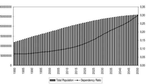
The Figure 1 below presents the IBGE population projections and the dependency ratio from 1980 until 2050. The dependency ratio is defined by the number of individuals aged 65 and above by the number of individuals aged 15 to 64.

The dependency ratio is expected to increase along the time but it is still inferior to those among more developed countries. The Table 1 below shows these figures for some selected countries.

7_{Supposing that}_g_{is the labor productivity growth, “(. . . ) if labour productivity grows at}_g_{% per year, so will real wages.}

Hence, the lifetime labour income of each new cohort will beg% larger than that of its immediate predecessor. So in assuming that each successive cohort pays lifetime net taxes that areg% larger than those of its predecessor, we are assuming that each successive future cohort pays the same share of its lifetime labour income in net taxes; i.e., we are assuming that each future cohort faces the same lifetime net tax rate.” (Cardarelli et al., 2000).

8_{Similar hypothesis were used by Holanda (2000) and Malvar (1999).}

(7)

Figure 1 –Population and Dependency Ratio

Source: IBGE

Table 1 –Population and Dependency Ratio: Selected Countries (1995) France Japan Norway New Zealand Population (Millions) 58 125.57 4.4 3.6 Dependency Ratio (elderly) 22.10% 22.21% 26.00% 19.50%

Source: Levy and Doré (1999); Takayama et al. (1999);Erling and Gjersem (1999); Baker (1999).

Henceforth, it is clear that the Brazilian dependency ratio is lower than the dependency ratio of the developed countries but it tends to increase sharply in the next decades. As mentioned above, the increases in this ratio elevate the government expenditures with health assistance and with retirement transfers: the amount of contributions falls relatively to the number of necessary transfers.

Our simulations will take into account part of this phenomenon – up to 2050 the IBGE data consider this trend. From 2050 on we assume two possible scenarios: (i) the basic scenario in which from 2050 on the population of each cohort will continue to increase at the 2050 growth ratio and (ii) the scenario without aging in which we use the constant population structure hypothesis – the dependency ratio will remain the same from 2050 on.

2.6. Government Consumption and Public Debt

(8)

sex profile of these taxes. After all these adjustments we reach a value of R$ 134.946.584.000,94. This value is projected until 2200 using the productivity growth rate and its present value is obtained using the assumed discount rates.

Regarding the public debt, the Figure 2 below presents its value (internal and external) of all gov-ernment levels from January 1995 to August 2004 as a proportion of GDP.

Figure 2 –Public Debt (% GDP)

Source: IPEADATA

We use in our basic scenario the value of the public debt observed in December 1996 that reached R$ 269.193.430.000,00.

2.7. Age and Sex Profiles

In order to construct the relative age-sex profiles we used the data from the Brazilian Household Survey (POF/IBGE) for the 1995/96 years.10 _{According to Cardarelli et al. (2000) the profiles}_{“(. . . ) are then}

used to construct the average net tax payment that each current generation has to pay to the government in the remaining lifetime (. . . ). They are relative as we normalize them with respect to the values of a 40-years old male, which is calibrated so as to match the aggregate values of each tax and transfers (in the base year and in the futures ones when we have official projections). The profiles are often very different for different sexes; (. . . ). It is therefore necessary to construct different profiles for the sexes, as government expenditure will be a function of the demographic split between man and women.”

Henceforth, following taxonomy similar to that proposed by Levy and Doré (1999), we have con-structed age and sex profiles for the taxes listed above:

(i) Property Taxes and Fees: based on ITR, IPVA, IPTU and various taxes (Municipal, State and Federal);

(9)

(ii) Consumption Taxes: given the consumption structure of the POF’s individuals we estimated the contributions of ICMS, IPI and PIS/COFINS;

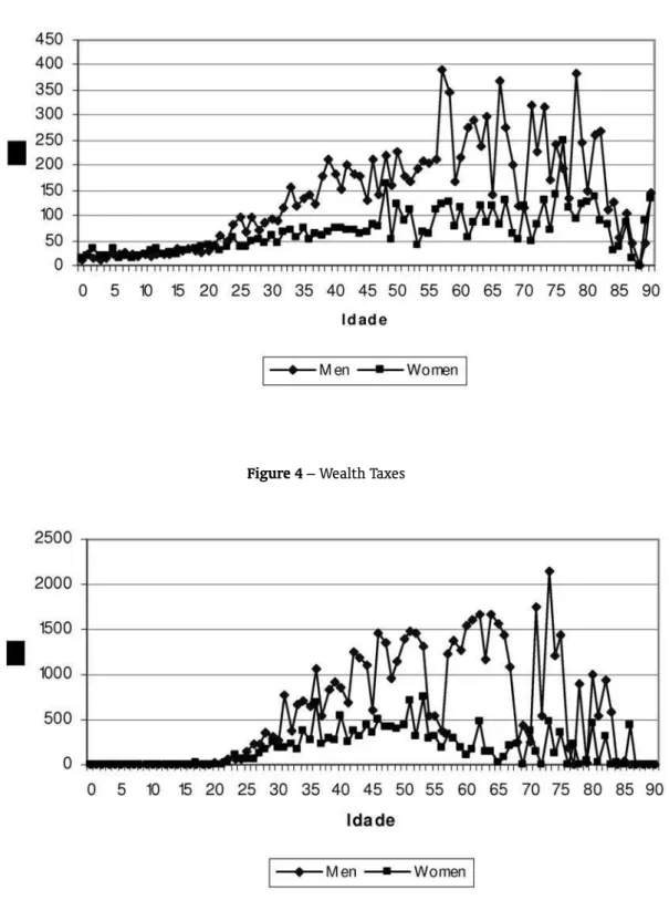
(iii) Wealth Taxes: for this profile we used the contributions of Wealth Tax and ISS declared by the POF’s individuals;

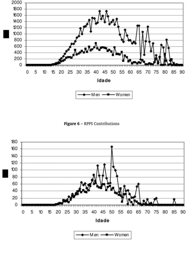
(iv) Social Security Contributions: this profile was based on the contributions for the Social Security (INSS and RPPS) and for the FGTS;

With regard to the transfers, we constructed the following age-sex profiles:

(i) Retirement Transfers: we obtained this profile considering the value of the retirement transfers paid by the government for the POF’s individuals; as we can not distinguish between a RPPS retired and a RGPS retired the profile based on retired transfers were used in both cases. This hypothesis is in accordance with Malvar (1999);

(ii) Other Transfers: This profile takes into account other social security transfers such as maternity insurance, insurance related to job accident, etc. and transfers from FGTS and PIS/PASEP;

(iii) Jobless Compensation: For this profile we also used the information on jobless compensation paid for the POF’s individuals;

(iv) Education: we obtained data on education from the Brazilian Education Ministry. In this case we distributed the expenditure with each education level equally to the individuals that indeed receive these transfers. Likewise, individuals aged from 0 to 6 years received equally the expenditure with basic education, the individuals aged from 7 to 14 received equally the expenditure with fundamental education and so on. This hypothesis is consistent with Malvar and Kotlikoff (1997). As mentioned above, we obtain these relative profiles dividing the payments of taxes and transfers of each cohort by the payment of the representative category of the model – the 40 years men. After-wards, based on the values effectively collected (paid) by the government – as stated in the Brazilian National Accounts – and on the projections of the population, we calibrated the 40 years individual contributions and, finally, we got the contributions of all cohorts.

Mathematically,

Hi,t = 90

a=0 (Pa,tm¯h

m a,i,t+P

f a,t¯h

f a,i,t)h

m

40,i,t (8)

In this equationHi,t is the total of the tax (transfer)icollected (paid) by the government at the

base year,Pm a,tand P

f

a,tare the populations of men and women of theayears old group at the base

year,¯hm

a,i,tand¯h f

a,i,tare the relative profiles of men and women of theayears old group at the base

year andhm

40,i,tis the profile of the forty years old man. This profile will be calibrated according to the

equation above:

Hi,t

90

a=0(P m

a,t¯hma,i,t+P f a,t¯h

f a,i,t)

=hm

40,i,t. (9)

(10)

Figure 3 –Property Taxes

(11)

Figure 5 –RGPS Contributions

(12)

Figure 7 –Consumption Taxes

(13)

Figure 9 –RPPS Transfers

(14)

Figure 11 –Other Transfers

(15)

3. THE GENERATIONAL ACCOUNTING RESULTS

3.1. The Basic Scenario

In this section we show the results for the basic scenario. Following the literature on Generational Accounting – see Auerbach and Kotlikoff (1999) – we assume a discount rate of 5% and a productivity growth of 1.5% and subsequently we check the robustness of the results using different values for these parameters. Besides, in the ongoing exercise we take into account the overall set of taxes collected and transfers paid for all levels of the Brazilian public administration. Table 2 below sums up the main results.

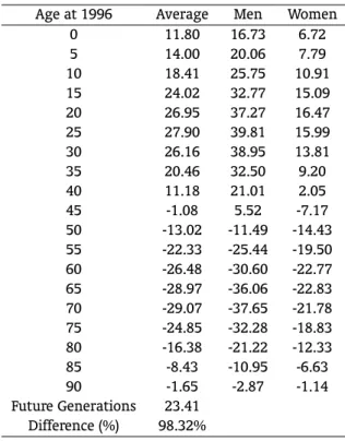
Table 2 –Generational Accounting of Present and Future Generations (R$Thousands) Age at 1996 Average Men Women

0 11.80 16.73 6.72

5 14.00 20.06 7.79

10 18.41 25.75 10.91 15 24.02 32.77 15.09 20 26.95 37.27 16.47 25 27.90 39.81 15.99 30 26.16 38.95 13.81

35 20.46 32.50 9.20

40 11.18 21.01 2.05

45 -1.08 5.52 -7.17

50 -13.02 -11.49 -14.43 55 -22.33 -25.44 -19.50 60 -26.48 -30.60 -22.77 65 -28.97 -36.06 -22.83 70 -29.07 -37.65 -21.78 75 -24.85 -32.28 -18.83 80 -16.38 -21.22 -12.33 85 -8.43 -10.95 -6.63 90 -1.65 -2.87 -1.14 Future Generations 23.41

Difference (%) 98.32%

According to this Table the lifetime net payments of the zero year cohort is, on average, R$11.800,00 in 1996 values. These payments increase sharply for the cohorts between 25-30 years old and start to reduce after the 30-35 years. This pattern is due to the prospective characteristics of the methodology: a thirty year individual is paying an expressive amount of all taxes and, on the other hand, he is relatively far from the retirement age which, in turn, tends to increase his net payments. Accordingly, for the individuals between 30-40 years old the net payments start to fall and become negative after the 45 years, indicating that these individuals are nearest the retirement age – or, in fact, they are retired – and are also paying less tax for the government.

(16)

merely the contributions made during a fraction of this time – which is the case for the individuals with one year or more in 1996.

We also considered the impacts of (i) the high public debt and of (ii) the aging of the Brazilian population upon these basic results. Table 3 shows the results for both the zero debt and the constant population structure scenarios.

Table 3 –Generational Accounting: Alternative Scenarios

Cohort 1996 Future Generations Imbalance

Basic Scenario 11.80 23.41 98.32%

Zero Debt 11.80 20.63 74.48%

Constant Population Structure 13.49 22.02 63.29%

Hence, supposing that the Brazilian public debt was zero, the imbalance would decrease almost 24% which is equivalent to say that the future generations would pay 74,48% more than an zero year old individual given the current fiscal rules. Alternatively, if we kept constant the age structure of the Brazilian population after 2050 – implying a constant dependency ratio after 2050 – the imbalance would be lesser: future generations, in these scenario, should pay 63,29% more than an individual born in the base year. Indeed, these considerations solely confirm that the debt and the population aging trend respond for a considerable fraction of the original imbalance.

Additionally, it can be useful to consider the extent of some fiscal policy measures that we need to achieve the intergenerational equilibrium. Table 4 and 5 below summarize some of these measures.

Table 4 –Tax Increases MEASURE VARIATION Wealth Taxes 69.29% Social Security (INSS) 56.65% Consumption Taxes 38.93% All Taxes 16.07%

Therefore, Table 4 shows that the Brazilian Government should increase wealth taxes in approxi-mately 70%, or raise the social security contributions for the INSS in 57%, or raise consumption taxes in 39% or, finally, increase all taxes in 16%. Alternatively, the necessary reduction in the public transfers is given below.

Table 5 –Spending Cuts MEASURE VARIATION Government Consumption 27.63%

Social Security (INSS) 51.44% Social Security (RPPS) 51.47% All Transfers 22.82%

(17)

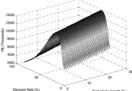
the graphics below we show how the main results vary when we change the discount rate and the productivity growth.11

The Figures above shed some light on the relation between the relevant parameters and the main results. Particularly, the third figure shows that when we give more weight to the future stream of net payments – either reducing the discounting rate or increasing the productivity growth of the economy – the generational imbalance rises sharply. However, even though the imbalance varies substantially with the parameters, the qualitative result of our analysis still persists: Brazilian intergenerational imbalance is positive for all pairs of discount rate and productivity growth considered in the current analysis.

Figure 13 –Sensitiveness Analysis: Zero Year Cohort

3.2. The Social Security System in the Basic Scenario

The impact of the social security imbalance on the general imbalance is also expressive. An as-sessment of these impacts can be done excluding from the basic scenario (Table 2) (i) the contributions and the transfer of RPPS, (ii) the contributions and the transfers of RGPS and (iii) the contributions and transfers of these two systems simultaneously.12The results are summarized below.

According to these results the exclusion of the private sector social security (RPPS) would cause a reduction of 30% (approximately) on the generational imbalance. On the other hand, the exclusion of the civil servants system (RPPS) implies an inversion in our results: in this case, present generations would be contributing substantially more than the future generations. The third column of the Table

11_{The Tables in the appendix show the results for alternative rates.}

12_{We defined the amount of contributions of RGPS and RPPS based on the concepts used by the Brazilian National Accounts}

(18)

Figure 14 –Sensitiveness Analysis: Future Generations

(19)

Table 6 –Generational Accounting: Social Security Age at 1996 Average

with-out RGPS

Average with-out RPPS

Average with-out both Sys-tems

0 10.66 17.83 16.69

5 12.30 20.82 19.11

10 15.68 25.62 22.89

15 20.39 32.05 28.42

20 22.91 36.47 32.43

25 24.28 39.02 35.40

30 24.21 39.10 37.16

35 21.68 35.65 36.87

40 16.88 29.28 34.97

45 10.25 20.47 31.80

50 3.79 11.51 28.31

55 -2.09 3.59 23.83

60 -5.08 -0.61 20.80

65 -8.35 -4.84 15.78

70 -9.50 -7.03 12.54

75 -8.82 -7.29 8.74

80 -5.75 -4.87 5.77

85 -3.11 -3.08 2.23

90 -0.57 -0.57 0.51

Future Generations 18.08 1.75 -3.58 Difference (%) 69.57% -90.20% -121.47%

shows the generational imbalance when these two systems are simultaneously excluded from the basic scenario.

Indeed, if we take into account only the social security taxes and transfers of each system we can conclude that the imbalance in Brazilian social security is substantial and deserves special attention from the policy makers. In the following exercises we consider only the numbers from RGPS and the numbers from the RPPS in order to assess the intergenerational imbalance of these systems. In other words, for the RGPS, we work with (i) the amount of INSS payroll taxes, (ii) the amount of INSS transfers and (iii) the government expenditure with investment and wages. Assuming that the debt of the sys-tem is zero, we can apply the Generational Accounting methodology for the RGPS. This procedure can analogously be reproduced for the RPPS case. Table 7 below presents the results.

(20)

Table 7 –Generational Accounting: Social Security (R$ Thousands)

(Average) RGPS RGPS RPPS RPPS

Age at 1996 Base GRGP S= 0 Base GRP P S

0 1.14 1.14 -6.02 -6.02

5 1.70 1.70 -6.82 -6.82

10 2.73 2.73 -7.21 -7.21

15 3.63 3.63 -8.03 -8.03

20 4.04 4.04 -9.52 -9.52

25 3.62 3.62 -11.12 -11.12

30 1.94 1.94 -12.94 -12.94

35 -1.22 -1.22 -15.19 -15.19

40 -5.70 -5.70 -18.10 -18.10

45 -11.32 -11.32 -21.55 -21.55

50 -16.81 -16.81 -24.52 -24.52

55 -20.24 -20.24 -25.92 -25.92

60 -21.40 -21.40 -25.88 -25.88

65 -20.62 -20.62 -24.13 -24.13

70 -19.57 -19.57 -22.04 -22.04

75 -16.03 -16.03 -17.56 -17.56

80 -10.63 -10.63 -11.51 -11.51

85 -5.32 -5.32 -5.35 -5.35

90 -1.08 -1.08 -1.08 -1.08

Future Generations 5.33 3.59 21.66 21.43 Difference (R$ Thousands) 4.19 2.45 27.69 27.45 Difference (%) 367.04% 214.99% -459.74% -455.78%

3.3. The Social Security Reforms

Given the dramatic situation of the social security systems – that became more apparent after the Real stabilization plan in 1994 – Fernando Henrique Cardoso and, recently, Lula governments has con-centrated considerable efforts on this issue.

First of all, in 1998 during the FHC mandate, the House of Representatives approved two important reforms.13 The intentions of the measures are twofold: (i) to reduce the disequilibrium in the RGPS through the imposition of a social security factor in the retirement transfers calculus and (ii) to reduce the disparities between the RPPS and RGPS through the introduction of a minimum age of retirement rule in the former system.

In other words, according to these measures:

(i) The retirement pensions from the INSS will be calculated based on a rule that takes into account the years of contribution of the individual, his age at the retirement moment and his life expectancy; (ii) The civil servants can retire only after 53 years old (men) and 48 years old (women).14 15

13_{Constitutional Amendment 20.}

14_{The factor is calculated according to the following equation:}_f ₌ Tca

Es(1 +

IdTca

100 ), whereTcis the number of contribution

years,ais the contribution rate (0,31),Esis the life expectancy of the worker at the retirement (IBGE) andIdis the worker’s age at the retirement.

15_{The minimum age rule also contained a transition rule. For further information see Zylberstajn and Afonso (2004) and}

(21)

Subsequently, during the Lula government another set of reforms was approved. The main points of these reforms are described below:16

(i) New RGPS ceiling;

(ii) Contributions from the civil servants: 11% over the values of the retirement pensions that exceed the RGPS ceiling;

(iii) New ceiling for the civil servants retirement pensions;

(iv) Minimum age rule: 60 years for men and 55 years for women plus a transition rule for the civil servants hired after 1998;

(v) Reduction in the RPPS pensions: 30% over the values that exceed the ceiling of R$2.400;

(vi) The end of the parity and integrality for the future civil servants: the benefits will be calculated according to the contributions;

In the Table below we present the impacts of some of these measures on the basic scenario and on the imbalance of the social security systems. More specifically, in the simulations we considered the following set of measures:

(i) Social security factor: we applied the average factor of 0.713 – which corresponds to the average age of retirement in this system (52 years) and to the average time of contribution (33 years) – on the benefits to be received for the individuals that, in the base year, aged less than 52 years (average age of retirement);

(ii) Minimum age for the civil servants: 53 years (men) and 48 years (women) –EC20. In these case, we simply imposed that the RPPS retirement pensions is equal to zero for the individuals that have not completed the minimum age requirements;

(iii) New RGPS ceiling: ten minimum wages – EC41. For the individuals paying contributions near the old ceiling, we raised these contributions up to the new ceiling. On the other hand, for the individuals receiving INSS transfers and aged less than 52 years, we also raised the transfers up to the new ceiling;

(iv) Minimum age for the civil servants: 53 years (men) and 48 years (women) –EC41.17 _{Again, we}

imposed that the RPPS retirement pensions is equal to zero for the individuals that have not com-pleted the minimum age requirements;

(v) Contribution of 11% from the civil servants: in this case, we also changed the RPPS contributions profile assuming that the individual contributions for this system is given by the new rule – and not by the “original” profile;

(vi) Contributions from the retired of RPPS: 11% over the retirement pensions that exceed the RGPS ceiling. In this case, the RPPS retirement transfer profile was changed according to this measure. In other words, the new profile considers that the individuals earning above the RPPS ceiling will pay 11% over the values that exceed the RPPS ceiling of ten minimum wages.

Bearing these considerations in mind, we present the results of the simulations in the Table below.

16_{Constitutional Amendment 41.}

17_{In this case, we took into account the transition rule assuming that the men would be retired after 57 years old and women}

(22)

Table 8 –Impacts of the Reforms on the General Imbalance Age at 1996 Basic

Sce-nario INSS Fac-tor INSS Ceil-ing FHC Mini-mum Age Lula Mini-mum Age Civil Servants Contr Retired Contr

0 11.80 12.64 12.65 13.44 14.18 14.47 14.51 5 14.00 14.95 14.96 15.91 16.79 17.14 17.18 10 18.41 19.42 19.44 20.55 21.58 21.99 22.04 15 24.02 25.15 25.17 26.48 27.69 28.17 28.22 20 26.95 28.28 28.34 29.87 31.29 31.86 31.92 25 27.90 29.45 29.52 31.31 32.99 33.65 33.71 30 26.16 27.95 28.02 30.09 32.08 32.82 32.90 35 20.46 22.55 22.62 24.94 27.30 28.14 28.22 40 11.18 13.65 13.71 16.33 19.15 20.14 20.24

45 -1.08 1.88 1.92 4.66 8.07 8.22 8.33

50 -13.02 -9.44 -9.41 -7.78 -3.81 -3.68 -3.54 55 -22.33 -22.33 -22.33 -22.33 -19.67 -19.56 -19.39 60 -26.48 -26.48 -26.48 -26.48 -26.48 -26.38 -26.18 65 -28.97 -28.97 -28.97 -28.97 -28.97 -28.91 -28.70 70 -29.07 -29.07 -29.07 -29.07 -29.07 -29.05 -28.83 75 -24.85 -24.85 -24.85 -24.85 -24.85 -24.84 -24.67 80 -16.38 -16.38 -16.38 -16.38 -16.38 -16.38 -16.26 85 -8.43 -8.43 -8.43 -8.43 -8.43 -8.43 -8.38 90 -1.65 -1.65 -1.65 -1.65 -1.65 -1.65 -1.65 Future Generations 23.41 21.11 21.05 18.65 15.97 15.18 15.04

Difference (%) 98.32% 67.04% 66.39% 38.75% 12.65% 4.89% 3.67% Marg. Effects (R$ Thousands) - -2.30 -0.06 -2.40 -2.68 -0.79 -0.13

Therefore, these results show that the social security reforms will have significant impacts on the Brazilian future generations. According to these estimates, the Brazilian generational imbalance will decrease from 98% to 3.67% – after the introduction of the reforms. This reduction is mainly given (i) by the minimum age rules and (ii) by the social security factor. With regard to this consideration, the last line of the Table shows the marginal effect of each measure on the future generations payments:18 _the

INSS factor will reduce the payments of the future generations in R$2.300, the INSS ceiling has a little effect on these payments, the minimum age rules reduce in R$2.400 (EC20 FHC) and R$2.680 (EC41 -Lula) the future generations payments and the other remaining measures reduce the future generations payments in R$790 and R$130, respectively.

We also present the impacts of these measures on both the RGPS and the RPPS imbalances.

In the RGPS case, the introduction of the factor causes a drastic reduction in the imbalance. The new INSS ceiling, as already mentioned, has insignificant impacts on the generational imbalance. Nev-ertheless, although these measures have drastically reduced the imbalance in this system, the future generation members will face a net contribution burden that is 49% higher than the burden faced by the current newborns.

18_{The marginal effect shows the “isolated” impact of the measure. For example, in the case of the minimum age, in the column}

(23)

Table 9 –The Impacts of the Reforms on the RGPS Imbalance Age at 1996 Basic Scenario INSS Factor INSS Ceiling

0 1.14 1.97 1.99

5 1.70 2.65 2.67

10 2.73 3.74 3.76

15 3.63 4.76 4.78

20 4.04 5.37 5.43

25 3.62 5.18 5.24

30 1.94 3.74 3.81

35 -1.22 0.87 0.93

40 -5.70 -3.22 -3.17

45 -11.32 -8.37 -8.32

50 -16.81 -13.23 -13.20

55 -20.24 -20.24 -20.24

60 -21.40 -21.40 -21.40

65 -20.62 -20.62 -20.62

70 -19.57 -19.57 -19.57

75 -16.03 -16.03 -16.03

80 -10.63 -10.63 -10.63

85 -5.32 -5.32 -5.32

90 -1.08 -1.08 -1.08

Future Generations 5.33 3.03 2.97 Difference (R$ Thousands) 4.19 1.05 0.98 Difference (%) 367.04% 53.40% 49.37% Marg. Effect (R$ Thousands) - -2.30 -0.06

The reforms also have a relevant impact on the RPPS: the difference between the current newborn payments and between the future generations’ payments that reached R$27.690 in the basic scenario decreases to R$19.820 after the reforms. However, the imbalance still persists: the future generations members has a burden R$20.000 higher than the members of the cohort born in the base year. In the INSS, for example, the difference after the reforms is R$980.

To sum up, it is possible to say that, even though the social security reforms have promoted the intergenerational balance in the public budgets, the imbalance in the RGPS and mainly in the RPPS persists. In other words, these results show that the Brazilian public sector will continue to collect huge amounts of taxes on wealth, on consumption and on property in order to afford the imbalance in his social security systems.

4. CONCLUSIONS

In this paper we used the Generational Accounting model developed by Auerbach et al. (1991) to study both the intergenerational imbalance of the Brazilian public budget and the intergenerational imbalance in the social security systems. Based on this methodology, a wide set of reforms in the social security systems approved by FHC and Lula governments were simulated and its impacts on the future and present generations were obtained.

(24)

Table 10 –The Impacts of the Reforms on the RPPS Imbalance Age at1996 Basic

Scenario FHC Min-imum Age Lula Min-imum Age Civil Ser-vants Contr Retired Contr

0 -6.02 -5.23 -4.50 -4.20 -4.16

5 -6.82 -5.87 -4.99 -4.64 -4.60

10 -7.21 -6.10 -5.07 -4.66 -4.61

15 -8.03 -6.72 -5.51 -5.03 -4.98

20 -9.52 -7.99 -6.56 -5.99 -5.94

25 -11.12 -9.33 -7.65 -6.99 -6.92

30 -12.94 -10.87 -8.88 -8.14 -8.07

35 -15.19 -12.87 -10.51 -9.67 -9.58

40 -18.10 -15.48 -12.66 -11.67 -11.57

45 -21.55 -18.81 -15.40 -15.26 -15.14

50 -24.52 -22.90 -18.92 -18.80 -18.66

55 -25.92 -25.92 -23.26 -23.15 -22.97

60 -25.88 -25.88 -25.88 -25.78 -25.57

65 -24.13 -24.13 -24.13 -24.07 -23.87

70 -22.04 -22.04 -22.04 -22.02 -21.80

75 -17.56 -17.56 -17.56 -17.55 -17.38

80 -11.51 -11.51 -11.51 -11.51 -11.40

85 -5.35 -5.35 -5.35 -5.35 -5.30

90 -1.08 -1.08 -1.08 -1.08 -1.08

Future Generations 21.66 19.27 16.58 15.79 15.66 Difference (R$ Thousands) 27.69 24.50 21.08 19.99 19.82

Difference (%) -459.74% -468.44% -468.83% -475.74% -476.07% Marg. Effect (R$ Thousands) - -2.40 -2.68 -0.79 -0.13

This imbalance is consistent with other results for the Brazilian economy – Malvar (1999) and Holanda (2000).

The imbalances in the RGPS and RPPS are even higher. With regard to this point, the net contribu-tions of a representative individual from the future generacontribu-tions to the RGPS is, on average, 367% higher than the net contributions of a current newborn. This is equivalent to say that an individual from the future generation should pay during his lifetime R$4.190 more than an individual born in 1996 in or-der to grant the solvency of the system. The RPPS situation is also complicated: a future generation individual must pay (in net contributions) R$27.690 more than a current newborn – given the RPPS inter-temporal budget constraint.

Indeed, the impact of the social security intergenerational imbalance on the global imbalance is substantial: the exclusion of the RGPS from our basic scenario would reduce the global imbalance from 98% to 69%, the exclusion of the RPSS would reduce this imbalance to –90% and the exclusion of both systems would reduce the imbalance to –121%. In other words, the extinction of these systems would invert thoroughly the imbalance. Given this scenario, the present generations would be contributing considerably more than the future generations what would allow the government to pursue an expan-sionist fiscal policy.

(25)

will continue to collect huge amounts of wealth, consumption and property taxes in order to afford the imbalance in his social security systems.

Bibliography

Afonso, L. E. & Fernandes, R. (2005). Uma estimativa dos aspectos distributivos da previdência social no brasil.Revista Brasileira de Economia, 59(3):295–334.

Altamiranda, M. F. (1999). Argentina’s generational accounts: Is the convertibility plan’s fiscal policy sustainable? In Allan J. Auerbach, L. K. e. W. L., editor,Generational Accounting around the World. The University of Chicago Press.

Auerbach, A. J. & Chun, Y. J. (2003). Generational accounting in korea. NBER Working Papers 9983, Na-tional Bureau of Economic Research, Inc. available at❤tt♣✿✴✴✐❞❡❛s✳r❡♣❡❝✳♦r❣✴♣✴♥❜r✴♥❜❡r✇♦✴

✾✾✽✸✳❤t♠❧.

Auerbach, A. J., Gokhale, J., & Kotlikoff, L. J. (1991). Generational accounting: A meaningful way to eval-uate fiscal policy. Journal of Economic Perspectives, 8(1):73–94. available at❤tt♣✿✴✴✐❞❡❛s✳r❡♣❡❝✳

♦r❣✴❛✴❛❡❛✴❥❡❝♣❡r✴✈✽②✶✾✾✹✐✶♣✼✸✲✾✹✳❤t♠❧.

Auerbach, A. J. & Kotlikoff, L. J. (1999). The methodology of generational accounting. In Allan J. Auerbach, L. K. e. W. L., editor,Generational Accounting around the World. The University of Chicago Press. Baker, B. (1999). Generational accounts in new zealand. In Allan J. Auerbach, L. K. e. W. L., editor,

Generational Accounting around the World. The University of Chicago Press.

Barreto, F. A. F. D. & Oliveira, L. G. S. (2001). Transição para regimes previdenciários de capitalização e seus efeitos macroeconômicos de longo prazo no brasil.Estudos Econômicos, 31(1).

Cardarelli, R., Sefton, J., & Kotlikoff, L. J. (2000). Generational accounting in the uk. Eco-nomic Journal, 110(467):F547–74. available at ❤tt♣✿✴✴✐❞❡❛s✳r❡♣❡❝✳♦r❣✴❛✴❡❝❥✴❡❝♦♥❥❧✴

✈✶✶✵②✷✵✵✵✐✹✻✼♣❢✺✹✼✲✼✹✳❤t♠❧.

de Góes Ellery Junior, R. & Bugarin, M. N. S. (2003). Previdência social e bem estar no brasil. Revista Brasileira de Economia, 57(1). available at❤tt♣✿✴✴✐❞❡❛s✳r❡♣❡❝✳♦r❣✴❛✴❢❣✈✴❡♣❣r❜❡✴✸✾✽✹✳❤t♠❧. Erling, S. J. & Gjersem, C. (1999). Generational accounts and depletable resources: The case of norway. In Allan J. Auerbach, L. K. e. W. L., editor,Generational Accounting around the World. The University of Chicago Press.

Ferreira, S. G. (2004). Social security reforms under an open economy: The brazilian case. Revista Brasileira de Economia, 58(3). available at❤tt♣✿✴✴✐❞❡❛s✳r❡♣❡❝✳♦r❣✴❛✴❢❣✈✴❡♣❣r❜❡✴✺✸✶✸✳❤t♠❧. Giambiagi, F., Mendonça, J. L. d. O., Beltrão, K. I., & Ardeo, V. L. (2004). Diagnóstico da previdência social

no brasil: O que foi feito e o que falta reformar? Discussion Paper 1050, IPEA.

Holanda, S. F. (2000). Impacto intergerações de mudanças em sistemas previdenciários – uma aplicação da “generational accounting” ao brasil. Master’s thesis, University of São Paulo.

Levy, J. & Doré, O. (1999). Generational accounting for france. In Allan J. Auerbach, L. K. e. W. L., editor,

Generational Accounting around the World. The University of Chicago Press.

Malvar, R. V. (1999). Generational accounting in brazil. In Allan J. Auerbach, L. K. e. W. L., editor,

(26)

Malvar, R. V. & Kotlikoff, L. J. (1997). Balanço intergeracional: O caso brasileiro. Pesquisa e Planejamento Econômico, 27(3):493–518.

Sanches, F. A. M. (2005). Balanço intergeracional: Desequilíbrio fiscal e reforma da previdência no brasil. Master’s thesis, University of São Paulo.

Takayama, N., Kitamura, Y., & Yoshida, H. (1999). Generational accounts in japan. In Allan J. Auerbach, L. K. e. W. L., editor,Generational Accounting around the World. The University of Chicago Press. Zylberstajn, H.; Souza, A. P. & Afonso, L. (2004). O sistema previdenciário brasileiro: Diagnóstico e

impactos fiscais das reformas recentes. University of São Paulo, mimeo.