Decision trees for loss prediction in retail - case of Pingo Doce

i

DECISION TREES FOR LOSS PREDICTION IN RETAIL

Mariana Bonito Henriques

Case of Pingo Doce

Project Work presented as the partial requirement for

obtaining a Master’s degree in Information Management

ii

NOVA Information Management School

Instituto Superior de Estatística e Gestão de Informação

Universidade Nova de Lisboa

DECISION TREES FOR LOSS PREDICTION IN RETAIL

Case of Pingo Doce

Mariana Bonito Henriques

Project Work presented as the partial requirement for obtaining a Master’s degree in Information Management with specialization in Knowledge Management and Business Intelligence

Advisor: Professor Doutor Roberto André Pereira Henriques

iii

ABSTRACT

The use of data mining as a way of solving problems from the widest range of areas with the main purpose of gaining competitive advantage is rising, specially in retail, an extremely competitive sector that requires an even bigger advantage. Additionally, food loss, beyond representing a huge waste of resources, can also be considered a major issue to the retail sector due to the financial losses originated from it. Thus, I proposed to help Pingo Doce, a well-known Portuguese retail company, to solve their food loss issue which, despite being the major cause of a huge drop in the company’s profits, has never been solved till this day.

Therefore, this project focuses on the development of a classification algorithm that will allow to predict future significant losses in several fruits sold in certain Pingo Doce stores. To do so I applied a Decision Tree algorithm that, due to its representation in the form of if-then rules, will help to identify the main features that lead to a higher number of losses, namely the period of the year and the category to which each fruit belongs, among others.

The dataset provided by the company contains variables that measure the quantity and value of sales, stocks, identified and unidentified losses, over a one-year period, and regarding 81 different fruits and 20 stores from all over the country. Additionally, I created new variables such as the criminality rate of the municipality and the climate class of each store, as well as the seasons and the day of the week in which each observation occurred. All these variables allowed me to create four different datasets that originated four different Classification Trees.

The results show that, using a dataset with no information regarding stocks and sales, containing only variables that describe the characteristics of the stores, products and periods of time, as well as the value of product sold per unit of measurement, i.e. the price per unit of measurement of each fruit, it is possible to create a Decision Tree that reaches an accuracy of 74% and correctly predicts 82% of the observations that represent significant losses.

The algorithm obtained allowed to identify the variables that are more prone to originate significant losses, namely: the day of the week, the fruit’s category, the season of the year, the position of that week in the respective month and the price at which the product is being sold.

KEYWORDS

iv

INDEX

1.6.Introducing The Company ... 2

2. LITERATURE REVIEW ... 4

2.1.Data Mining ... 4

2.2.Data Mining in the Retail Sector ... 5

2.3.Machine Learning ... 6 2.4.Decision Trees... 7 2.4.1.Definition ... 7 2.4.2.Advantages ... 7 2.4.3.Method ... 8 2.4.4.Splitting criteria ... 8 2.4.5.Overfitting ... 9 2.4.6.Stopping criteria ... 9 2.4.7.Algorithms ... 9 2.5.Measuring Performance ... 10 2.5.1.Accuracy ... 11

2.5.2.Sensitivity and specificity ... 11

2.5.3.Precision and recall ... 12

2.5.4.F-measure ... 12

2.6.Cross-Validation ... 12

3. METHODOLOGY AND TOOLS ... 13

3.1.Business Understanding ... 13

3.2.Data Understanding ... 13

3.2.1.Descriptive Analysis ... 14

v 3.3.Data Preparation ... 24 3.3.1.Data import ... 24 3.3.2.Data cleaning ... 24 3.3.3.Data transformation ... 29 3.3.4.Data reduction ... 33 3.4.Modeling ... 37 3.5.Evaluation ... 39

4. RESULTS AND DISCUSSION ... 40

4.1.Model 1 – tese_NoCorr ... 40

4.2.Model 2 – tese_PCA ... 40

4.3.Model 3 – tese_ChosenVar1 ... 40

4.4.Model 4 – tese_ChosenVar2 ... 40

5. CONCLUSIONS ... 42

6. LIMITATIONS AND RECOMENDATIONS FOR FUTURE WORK ... 44

7. BIBLIOGRAPHY ... 46

8. ANNEXES ... 49

vi

LIST OF FIGURES

Figure 2.1: Volume of data created worldwide from 2010 to 2025, in zetabytes ("Data created

worldwide 2010-2025 | Statista", 2019) ... 4

Figure 3.1: Boxplot of the Venda Valor Unitário Médio variable ... 16

Figure 3.2: Stock Cobertura formula ... 18

Figure 3.3: Sum of the quantity of identified losses, per month ... 19

Figure 3.4: Sum of the quantity of unidentified losses, per month ... 20

Figure 3.5: Number of observations per category of product ... 21

Figure 3.6: Number of observations per month ... 23

Figure 3.7: Number of observations per week ... 23

Figure 3.8: Number of observations per day ... 24

Figure 3.9: Number of instances with an unidentified loss quantity different than zero, per week ... 33

Figure 3.10: Correlation Matrix of the transformed dataset ... 35

Figure 3.11: Plot of the Cumulative Sum of the Explained Variance per Number of Components ... 36

Figure 3.12: DT built from the ChosenVar1 dataset, with maximum depth of 3 ... 38

Figure 8.1: DT built from the tese_ChosenVar1 dataset, with maximum depth of 4 ... 49

Figure 8.2: DT built from the tese_ChosenVar2 dataset ... 50

vii

LIST OF TABLES

Table 2.1: Meaning of each measure ... 10

Table 2.2: Confusion Matrix ... 11

Table 2.3: Summary of each Evaluation Measure formula ... 12

Table 3.1: Meaning of each variable of the original dataset ... 15

Table 3.2: Summary of the statistical analysis of the four sales related variables ... 17

Table 3.3: Summary of the statistical analysis of the stock related variables ... 18

Table 3.4: Summary of the statistical analysis of the four losses variables ... 20

Table 3.5: Summary of the analysis of the non-numerical variables ... 21

Table 3.6: Top 10 of the most mentioned articles ... 22

Table 3.7: Number of outliers using the Z-score method, grouped by variable and category of product ... 26

Table 3.8: Summary of the new variable’s formula ... 30

Table 3.9: Criminality Rate of each store ... 30

Table 3.10: Average of the Quebra Total variable, per category of product ... 31

Table 3.11: Removed variables and respective reason for removal ... 34

Table 3.12: Summary of the four created datasets ... 36

Table 3.13: Detail on the input variables of the tese_ChosenVa1 and tese_ChosenVar2 datasets ... 37

viii

LIST OF ABBREVIATIONS

1

1. INTRODUCTION

1.1. C

According to (Jagdev, 2018), retailers are now mining customer data to increase profits and growth, as well as to be in competition, allowing them to reach an increase in sales in more than 70%. Therefore, the exponential growth of data in the retail sector (Jagdev, 2018) presents unique opportunities to its holders to create information, and therefore knowledge, with the purpose of obtaining advantage towards their competitors (Davison & Weiss, 2010). Although originally the process of turning data into knowledge relied on manual analysis (Fayyad, Piatetsky-Shapiro, & Smyth, 1996), nowadays we are capable of “discovering useful patterns and trends in large data sets”, by the appliance of several technologies and techniques (Larose & Larose, 2014, Chapter 1, para. 4).

That said, retailers should rely on Data Mining to access and analyse their data, not only to achieve better results, but also to obtain a better understanding of both their customers and their operations (Jagdev, 2018).

1.2. P

According to (Daryanto & Sahara, 2016), food loss, which occurs both at wholesale and retail markets, represents a problem since it not only contributes to financial losses but also to the waste of natural resources. Although there is no agreement on the quantity of currently lost global food production, fresh fruits and vegetables are among the products with a higher percentage of food waste (Parfitt, Barthel, & MacNaughton, 2010). Despite the difficulty to measure this proportion it is estimated that “worldwide about one third of all fruits and vegetables produced are never consumed by humans” (Kader, 2005).

Since a high number of losses leads to a strong decrease in the net income attributable to the company, in comparison with the value that would be expected given the number of stored products in each store, and once this is a recurrent problem in all Pingo Doce stores, it results in a significant decrease in the revenue of the company. Additionally, given the competitive nature of retail, this unnecessary decrease in the revenue must be eliminated or at least reduced so that it won’t be a disadvantage to this company.

Given the fact that food loss in Pingo Doce is more common in fresh products such as fruits and vegetables, the company decided that it is a priority to start by analysing the losses that occur in those products. Consequently, in this project data mining techniques will be used to develop a model that will be able to predict if a significant loss will occur, more specifically in the fruit’s category, in several Pingo Doce stores.

1.3. M

As previously referred, losses induce a decrease in the net income of the company together with an increase in the food waste. Due to both reasons it is in the interest of everyone involved to find a solution to this problem. Solving this problem obviously results in a notable reduction in the number of significant losses, what would derive in a decrease in the quantity of wasted products, as well as in the value lost by the company. This would obviously be beneficial to the company since it would

2 increase their profit. Finally, solving this problem using Machine Learning algorithms would demonstrate how important this field is to retail companies, though most of them are not yet ready to take advantage of this useful techniques.

1.4. P

The proposal to solve this problem is to rely on Data Mining techniques by applying a supervised Machine Learning algorithm. This approach consists in performing not only data analysis but also discovery algorithms that create patterns or models over the data, allowing to predict whether certain article will suffer a significant loss or not, in a certain future time period, depending on the values observed in the variables available in the provided dataset.

Although machine learning algorithms are widely used and relatively simple to create and implement, and even though this is a huge company with thousands of employees with a lot of expertise, this process has never been used with the purpose of solving the losses issue. Additionally, as previously said, this is a huge concern to the company, which has already tried more than once to find a solution to this question, however always unsuccessfully. Therefore, the success of this project would be unprecedented, bringing great benefits to the company and consequently to the Jerónimo Martins Group.

1.5. O

The major objective of this work is to show the applicability of Machine Learning and Data Mining in the study of the high number of losses that occur in this company, and probably in all retail companies. Besides this major objective, I can also point out several smaller objectives such as: pre-processing the data that was provided, creating and applying several models to the pre-processed data, evaluating all models to figure out which presents the best results and present it to the company as the model that will help solving their problem.

1.6. I

T

C

Jerónimo Martins is an International Group with its headquarters in Portugal, founded in 1792 by a namesake young man from Galicia that decided to open a store in the downtown of Lisbon, soon becoming the main supplier of the portuguese capital. The business thrives until 1920, when on the verge of bankruptcy, the company is bought by a set of merchants from Porto called “Grandes Armazéns Reunidos”, who agreed to keep the name as “Estabelecimento Jerónimo Martins & Filho”. Among the five associates that formed the company, three eventually abandoned it, remaining only: Elísio Pereira do Vale and Francisco Manuel dos Santos. In 1945, Elísio Alexandre dos Santos, nephew of Francisco Manuel dos Santos, becames director of Jerónimo Martins, and after his death in 1968, the family business is assumed by his son Alexandre Soares dos Santos. Under the direction of Alexandre Soares dos Santos, the supermarket chain Pingo Doce is founded in 1978, with the opening of the first Pingo Doce store in 1980. Fifteen years later, in 1995, the group started its internationalization, firstly with the expansion to Poland and finally in the year of 2013 with the opening of the first Ara stores in Colombia. Therefore, this is a group with 227 years of experience as a Food Specialist, that nowadays is present in three geographies, namely Portugal, Colombia and Poland, in two different continents, counting with more than 104 000 employees and over 3 600 stores.

3 Currently, Jerónimo Martins’ Group structure is divided in two major areas: Food Distribution and Specialized Retail. Examples of the first mentioned area are: Pingo Doce and Recheio in Portugal, Biedronka in Poland and Ara in Colombia. Regarding the Specialized Retail area there are examples like Jeronymo and Hussel in Portugal and Hebe, a chain of specialized Health and Beauty stores, in Poland. In Portugal, Jerónimo Martins´ businesses in Food Distribution have two main strands: Pingo Doce, as a food retail company, and Recheio Cash & Carry, as wholesale food company.

This project was developed in partnership with Pingo Doce, since among all the portuguese companies belonging to the Jerónimo Martins Group this is the one that presents the biggest number of losses. The remaining of this document follows the according structure: the next chapter contains the literature review and the subsequent chapter presents the methodology used in this project. Thereafter, chapter 4 is assigned to the presentation of results and respective discussion, chapter 5 introduces the conclusion of the project and lastly, in chapter 6, the project limitations are mentioned together with several recommendations for future works.

4

2. LITERATURE REVIEW

2.1. D

M

The amount of data created worldwide is growing exponentially through the years (Davison & Weiss, 2010). According to the graphic presented below (Figure 2.1), which reflects the increase in the amount of data created worldwide from 2010 to 2025 ("Data created worldwide 2010-2025 | Statista", 2019), in 2010, 2 zetabytes of data were created worldwide, while in 2015 that number grew to more than 15 zetabytes. Moreover, the number of worldwide created data in 2020 and 2025 were predicted using forecasting methods, expecting to reach 175 zetabytes in 2025, which represents 87,5 times more data than the one created in 2010.

Figure 2.1: Volume of data created worldwide from 2010 to 2025, in zetabytes ("Data created worldwide 2010-2025 | Statista", 2019)

The tremendous growth in the data available, caused by the advances in computer technology, the emergence of high-speed networks and the diminishing of disk costs, represents a challenge, since traditional statistical techniques are not capable of handling such large amounts of data (Davison & Weiss, 2010). Additionally, the non-traditional nature of data together with its lack of structure makes it impossible to be analysed with the established data analysis techniques (Tan, Steinbach & Kumar, 2005). Due to all these reasons, manual data analysis became no longer sustainable and several new methods, tools and technologies were required to support humans in extracting information from all the accessible data (Fayyad et al., 1996), resulting in the creation and development of the field of Data Mining (Tan, Steinbach & Kumar, 2005). Consequently, data mining appeared as a “technology that

blends traditional data analysis methods with sophisticated algorithms for processing large volumes of data” (Tan, Steinbach & Kumar, 2005, p. 1), allowing to automatically recognize useful patterns, and

5 Therefore, DM tasks can be divided into two main categories (Davison & Weiss, 2010), namely: description, that summarizes the data in some way, perhaps by segmenting data based on similarities and differences observed (Chen et al., 2012), and prediction, that allows to predict the value of a future observation by finding patterns in data that allow to estimate the future behaviour of some entities (Fayyad et al., 1996). Inside the prediction task we can distinguish two of the most commonly used DM tasks: classification and regression, bearing in mind that both tasks entail the creation of a model that predicts a target variable from a set of explanatory variables (Davison & Weiss, 2010). While in classification a function that maps a data item into one of several predefined classes is learned, in regression the applied function maps data items to a real-valued prediction variable (Fayyad et al., 1996).

In this project I will rely on classification since my objective is to predict if a certain product will suffer a significant loss, belonging to one of this two possible classes.

2.2. D

M

R

S

The challenge of managing huge amounts of data and the capability of recognizing the relevant information from it, together with the need for immediate product and service development that allows to take advantage of freshly market opportunities are some of the factors that have contributed for the imperative need to adopt data mining tools for companies that want to differentiate themselves from their competition and gain a good position in today’s market (Kleissner, 1998). Therefore, data mining solutions are used to assist critical decision making in several areas such as banking, not only for fraud and money laundering detection (Raj, 2015) but also for loan credibility prediction trough the use of a Decision Tree that identifies the most significant customers’ characteristics for credibility supporting banks in the process of decision making regarding loan requests (Sudhakar & Reddy, 2016); healthcare, trough the development of efficient heart attack prediction methods (K, M, & R, 2018); and transportation industries, allowing planners to better perceive public transport user behaviours, thus helping to improve their service (Agard, Morency, & Trépanier, 2006).

Lastly, the Retail area should be emphasized once it is the one being analysed in this project. Being defined as “the activity of selling goods to the public, usually in shops” ("RETAIL | Meaning, definition in English Dictionary", 2019), it allows and enhances the use of several DM mechanisms with the purpose of determining what kind of products a customer usually purchases at the same time or even to create targeted marketing campaigns to different clusters of customers, achieved through the definition of groups of customers that present similar characteristics (Kleissner, 1998), as presented in (Chen et al., 2012) where a Recency, Frequency and Monetary model was used with the purpose of dividing the customers of an UK-based online retailer into several meaningful groups through the use of the k-means clustering algorithm, clearly identifying the main characteristics of the consumers in each group. Therefore, many online retailers like Amazon, Walmart, Tesco and EasyJet are already applying data mining techniques with the purpose of supporting customer-centric marketing, allowing them to benefit from a competitive advantage (Chen et al., 2012).

Another example of the use of data mining in retail industry is the improvement of future stock estimate by the analysis of several datasets regarding sales with the objective of predicting alterations

6 in demands, as presented in (Manyika et al., 2011), where retailers rely on bar code systems data to automate stock replenishment, cutting down the number of incidents of stock delays.

Additionally, in (Zhang, Cheng, Liao, & Choudhary, 2012), customer reviews from Amazon’s website were analysed trough the use of a model that returned each product ranking result by: filtering each review’s content and removing unrelated comments, assigning weights to each review based on its helpfulness and time since posting date and calculating each product’s ranking score by combining the previous weights to the polarity of each review, i.e. the difference between the number of positive and negative sentences that compose the review.

Finally, in (Karamshuk, Noulas, Scellato, Nicosia, & Mascolo, 2013) the extraction of knowledge from geographic data towards services improvements was studied. In the mentioned work, a dataset from Foursquare, a location-based social network, was analysed with the objective of identifying the most promising area to open a new store among a set of pre-defined ones. This study was focused on three retail chains, namely Starbucks, McDonald’s and Dunkin’ Donuts, and a square region around the centre of New York and allowed to identify which geographic and mobility features are the best indicators of popularity for each retailer brand.

2.3. M

L

After introducing the concept of DM, I find it worth mentioning Machine Learning, since this project is based on predicting whether there will be a significant loss in certain products, through the application of ML algorithms. Therefore, considering the strong relationship between both concepts, making these definitions similar and therefore sometimes confusing, I find it imperative to present the concept of ML. As previously stated, DM can be defined as the “nontrivial extraction of implicit, previously

unknown, and potentially useful information from data” (Sahu, Shrma, & Gondhalakar, 2008, p. 114)

but the process of mining knowledge from data requires a technology that is able to provide tools that support it: Machine Learning (Witten, Frank, Hall, & Pal, 2016).

That said, and according to (Alpaydin, 2010, p. xxxi), ML can be defined as the process of “programming

computers to optimize a performance criterion using example data or past experience”. According to

(Shalev-Shwartz & Ben-David, 2013), ML can be divided into several subfields, depending on the nature of the interaction that occurs during the learning task. Consequently, we can distinguish two major types of machine learning algorithms: supervised learning algorithms, in which the inputs are given with the corresponding outputs, and unsupervised learning algorithms, in which every instance in the dataset is untagged (Kotsiantis, 2007). This allows us to understand that supervised methods have the objective of understanding the relationship between the predictor variables and the target variable (Rokach & Maimon, 2014), what is exactly the objective of this project. That said, since all instances in our dataset are labelled as 0 or 1 regarding the Significant Loss variable, allowing the algorithm to rely on that label to create a function that maps inputs to expected outputs, being able to classify new instances regarding their target variable value, I will apply supervised learning algorithms.

Supervised models can be divided into Regression and Classification models, depending on the domain of the target variable, since in regression the target variable has a real-valued domain while in classification the input space is projected into previously defined classes (Rokach & Maimon, 2014). According to this distinction, since my objective is to assign unlabelled instances into one of the two

7 possible classes regarding the Significant Loss variable (0 or 1), I can easily conclude that I am dealing with a classification problem, where supervised learning is frequently used (Oladipupo, 2010). Among the several supervised machine learning algorithms available for classification problems such as Support Vector Machine, Naïve Bayes Classifiers, Decision Trees, Neural Networks (Oladipupo, 2010), I decided to apply Decision Trees, since I found this the most suitable for the company’s problem due to its simplicity and self-explanatory nature, making its use and interpretation very accessible, even for non-data mining experts (Rokach & Maimon, 2014). Furthermore, this is a method with a fast learning process, contrarily to Neural Networks for instance (Podgorelec, Kokol, Stiglic, & Rozman, 2002).

2.4. D

T

2.4.1. Definition

Decision Trees are tree-shaped structures that are capable of classifying observations trough the analysis of its variables (Kotsiantis, 2007), representing “one of the most promising and popular

approaches” (Rokach & Maimon, 2014, p. ix) for the data mining process.

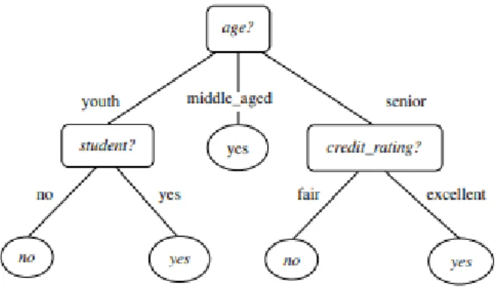
With roots from logic, management and statistics, DTs are a very accessible yet accurate tool to perform prediction, since it allows to easily describe and interpret the relationship between all features and the target variable values. This model can be used both for classification and regression, being respectively called a CT or RT (Rokach & Maimon, 2014). In this project, as already stated, I am dealing with a classification problem, which is why I will rely on a CT as the one presented below.

Figure 2.2: Example of a Classification Tree for the target variable buys_computer (Han, Kamber & Pei, 2012)

2.4.2. Advantages

The DT algorithm presents several advantages such as being simple and easy to interpret, due to its representation in the form of if-then rules, as well as its higher speed of classification, when compared to KNN and Naïve Bayes in classifying medium and large datasets (Jadhav & Channe, 2016). Additionally, despite being a straightforward method it can reach the same accuracy of the Back-Propagation Network when performing classification (Vafeiadis, Diamantaras, Sarigiannidis, & Chatzisavvas, 2015).

8 Considering the previously mentioned advantages I decided DT would be a good option to develop this project.

2.4.3. Method

In the DT algorithm the partitioning of data is usually achieved by successive partitions based on the values of the several explanatory variables, since each parent node will always be split and each child node will also become a parent node, unless it is a leaf (Moisen, 2008).

A tree always begins at the root node, being this the predictor variable that best splits the training data, according to the chosen method for finding this feature (Kotsiantis, 2007). The root node is the only with no incoming edges, while all the other nodes have exactly one incoming edge. All nodes that contain outgoing edges are called internal nodes, while the ones without outgoing edges are called terminal nodes or leaves (Rokach & Maimon, 2014). Each node corresponds to a variable of an instance, and each branch or edge represents a value or range of values that the variable can assume (Kotsiantis, 2007), always taking into account that the range of values must be “mutually exclusive and

complete” (Rokach & Maimon, 2014, p. 13), so that each instance of data can be mapped.

Each observation is classified starting at the root node and arranged depending on their predictor variables values (Kotsiantis, 2007) . That said, this algorithm starts by analysing the value of the feature that represents the root node, deciding to which branch this value belongs and moving on to the node that comes after the followed branch. This process is repeated until the algorithm reaches a leaf node (Rokach & Maimon, 2014).

2.4.4. Splitting criteria

As previously mentioned, the root node as well as the remaining nodes are chosen by applying a method that identifies the variable that best splits the data, by minimizing each node impurity, which is the same as maximizing its homogeneity (Kotsiantis, 2007). In a classification problem, the two most common impurity-based methods are Information Gain and Gini Index. While the first one uses Entropy as the impurity measure, the second one measures the divergences between the probability distributions of the target variable values (Rokach & Maimon, 2014).

According to the Information Gain method, the attribute with the highest value is chosen to split the node that is being analysed, since Information Gain represents the difference between the original information needed and the information needed if we split on a certain variable. This mentioned information represents the amount of information that is required to classify an instance in a certain partition and can also be named as entropy of that partition. By calculating the entropy of the original partition and the entropy after the partition using a specific attribute, we can calculate the Information Gain (Han, Kamber & Pei, 2012). That said, it is easy to conclude that the selected attribute will be the one that has the higher information gain that is obviously the one with the lowest entropy value. In the Gini Index splitting rule the algorithm isn’t measuring the information gain of the partition but rather its impurity. Since we want to minimize the impurity of each partition, the attribute that will be chosen to split a certain partition is the one that originates the maximum reduction in impurity, in other words: the one that has the minimum Gini Index_. Using this splitting criteria means that the tree will be created by binary splits (Han, Kamber & Pei, 2012).

9 In the lack of a splitting criteria that has a better performance than the remaining ones, and taking into account that the method chosen won’t make significant difference on the CT performance (Rokach & Maimon, 2014), I decided to try both splitting rules in order to understand which would bring the best evaluation measures.

2.4.5. Overfitting

Since the nodes that result from the root are also divided into more nodes, as well as all the following ones, the tree can outgrow and reach the point where it reflects the training data, sometimes dividing one instance per leaf, resulting in overfitting (Moisen, 2008). Overfitting happens when the classifier is a perfect fit of the training data, not being able to generalize to instances that are not part of the training (Rokach & Maimon, 2014) and consequently returning poor predictions (Moisen, 2008). According to (Kotsiantis, 2007, p. 252), a DT overfits the training data if another tree exists with a larger error than the original one when tested on the training but a smaller error when tested in the whole dataset. Furthermore, the complexity of a DT has a huge influence on its accuracy and on its comprehensibility (Rokach & Maimon, 2014), meaning it is crucial to identify the most suitable tree size.

There are two ways of identifying optimal tree sizes and therefore preventing overfitting, namely: not splitting a node if a defined threshold for the reduction in the node impurity isn’t reached or completely grow the tree and then prune unnecessary nodes until the it reaches an appropriate size (Moisen, 2008). While the first method represents a pre-pruning approach, the second one is called post-pruning. Although it is not possible to identify the best pruning method, pre-prune the DT by defining a stopping criteria to its growth can be recognized as the “most straightforward way of

tackling overfitting” (Kotsiantis, 2007, p. 252). 2.4.6. Stopping criteria

A tree grows until a stopping criteria is reached. While rigid stopping criteria will lead to an underfitted DT, unconstrained ones create large and overfitted trees. Some of the most frequently used stopping rules are: the maximum tree depth is reached, the number of instances in a node is smaller than the minimum number of instances required for parent nodes, the split of a node makes the number of instances in one of the child nodes smaller than the minimum required number of instances per child node, and finally if the best splitting criteria doesn’t reach the threshold for the reduction in a node’s impurity value (Rokach & Maimon, 2014).

2.4.7. Algorithms

According to (Rokach & Maimon, 2014), there are several DT algorithms, being ID3, C4.5 and CART the most common ones, all of them mostly differing in terms of splitting and stopping criteria. ID3 can be pointed out as the simplest of all above mentioned algorithms, relying on information gain as a splitting criterion and only stopping when all observations belong to a unique value of the target variable or the best information gain is equal or less than zero. This algorithm has several drawbacks, namely: not handling numeric features nor missing data and not using any pruning strategies, leading to overfitting. For all the previously specified disadvantages, and since the C4.5 algorithm can be considered an upgrade of the ID3, the C4.5 is preferred. This more evolved algorithm performs error-based pruning and handles both numeric and missing data. C4.5 uses gain ratio as a splitting criterion and only stops when the number of observations to split is below a defined threshold. The last of the three mentioned

10 algorithms, CART (Classification and Regression Trees) is known for creating binary trees, since each node has exactly two outgoing branches, being also able to generate regression trees since it supports numerical target variables. This algorithm uses Twoing, or prediction squared error in case of the regression trees, as splitting rules and performs Cost-Complexity pruning. From all available algorithms to create DT, C4.5 is considered the most popular in all literature (Kotsiantis, 2007). Although the algorithm available in scikit-learn is an improved version of the CART it can’t deal with categorical variables, at least for now, which implies that all non-numerical variables of the provided dataset will need to be transformed.

2.5. M

P

After defining which algorithm I will rely on to create my CT, it is important to identify a set of measures that allow me to evaluate the predictive performance of the created classifiers, with the objective of determining which model is the best at predicting the class of the target variable. These evaluation measures are calculated not only using the training data but also the test data, since we want to measure the model’s performance on new data, that was not used to create the classifier (Han, Kamber & Pei, 2012).

Among all the evaluation measures available to assess the predictive performance of CT, the most relevant are: accuracy, sensitivity, specificity, precision and f-measure (Rokach & Maimon, 2014). These evaluation measures are calculated using four simple variables, namely: True Positives, True Negatives, False Positives and False Negatives (Han, Kamber & Pei, 2012), whose meaning is presented in the table below (Table 2.1).

Measure Meaning in this project

True Positives (TP)

Number of instances in which the loss was significant, and the Significant Loss variable was correctly labelled as 1. True Negatives

(TN)

Number of instances in which the loss was not significant, and the Significant Loss

variable was correctly labelled as 0. False Positives

(FP)

Number of instances in which the loss was not significant, and the Significant Loss

variable was incorrectly labelled as 1. False Negatives

(FN)

Number of instances in which the loss was significant, and the Significant Loss variable was incorrectly labelled as 0.

Table 2.1: Meaning of each measure

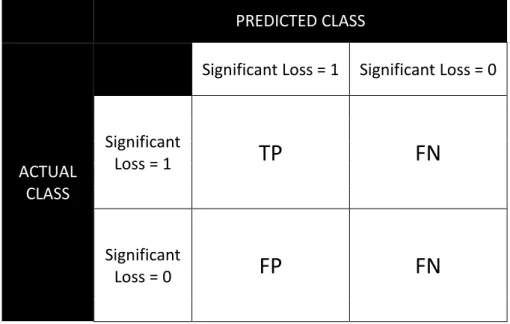
These four measures construct the Confusion Matrix (table 2.2), which helps in calculating all the initially referred evaluation measures that will be used to assess the model’s performance.

11 PREDICTED CLASS ACTUAL CLASS

Significant Loss = 1 Significant Loss = 0

Significant

Loss = 1

TP

FN

Significant

Loss = 0

FP

FN

Table 2.2: Confusion Matrix

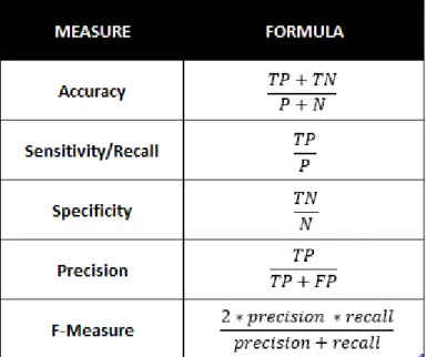
2.5.1. Accuracy

The accuracy measure represents the percentage of instances that were correctly predicted by the model among all the observations (Kotsiantis, 2007), indicating how well the classifier identifies instances of both classes (Han, Kamber & Pei, 2012). Although usually model’s evaluation is assessed mostly using the accuracy measure, it is not enough to perform a good evaluation, especially if the dataset has unbalanced classes’ distribution (Rokach & Maimon, 2014).

2.5.2. Sensitivity and specificity

Since accuracy is a function of sensitivity and specificity (Han, Kamber & Pei, 2012), these last two measures can be used, instead of the first one, each time the dataset is unbalanced (Rokach & Maimon, 2014).

Sensitivity, also called TP rate, is the percentage of positive instances that are correctly classified (Han, Kamber & Pei, 2012). Therefore, this measure, that can also be named Recall, represents how good the model is in identifying instances that belong to the positive class, that is instances with a Significant Loss value equal to 1 (Rokach & Maimon, 2014). Consequently, in this project, sensitivity will return the number of instances correctly classified as a significant loss divided by all the actual observations that have a significant loss.

In its turn, Specificity or TN rate, returns the percentage of negative instances that are correctly classified (Han, Kamber & Pei, 2012), which represents how good the model is in identifying negative instances (Rokach & Maimon, 2014). Consequently, in this project, specificity represents the number of instances correctly classified as a not significant loss divided by all the actual observations that are not significant losses.

12

2.5.3. Precision and recall

Precision is an evaluation measure that returns the proportion of actual positive instances among all observation that were classified as positive (Rokach & Maimon, 2014), being considered a measure of exactness (Han, Kamber & Pei, 2012). In this project it represents the number of instances correctly classified as a significant loss divided by all the observations classified as a significant loss.

Recall, as already stated, is the same as Sensitivity.

A score of 1 in the precision or recall measures is not necessarily a good indicator. Furthermore, since the relationship between both measures is inverse, allowing to increase one measure but at the cost of decreasing the other, a good approach to use these two measures is to combine them into a unique one which is called F-measure (Han, Kamber & Pei, 2012).

2.5.4. F-measure

The last evaluation measure I will use is called F-measure and represents the trade-off between Precision and Recall (Rokach & Maimon, 2014), since it returns the harmonic mean of these two measures, giving equal weight to both.

Table 2.3: Summary of each Evaluation Measure formula

2.6. C

-V

To assess the evaluation measures of the classifiers I used 10-fold cross-validation. In this method the original data is randomly divided into 10 mutually exclusive sets with approximately the same number of instances and training and testing phases are carried out 10 times, using 9 of the 10 sets as training data and the remaining as test data for each one of the 10 iterations. By following this approach, we guarantee that each instance is used 9 times for training and 1 for testing, obtaining an accuracy that represents the number of correctly classified instances from the 10 iterations divided by the total number of instances (Han, Kamber & Pei, 2012).

13

3. METHODOLOGY AND TOOLS

Despite the lack of a standard framework to guide the deployment of DM projects (Wirth & Hipp, 2017), we can name more than one methodology for this purpose, such as SEMMA and CRISP-DM, which are considered the most popular since their common use in several publications regarding DM (Azevedo & Santos, 2008).

On the one hand, to present the core process of conducting a data mining project, we can mention SEMMA. According to the SAS Institute, responsible for the SEMMA development, the acronym stands for: Sample, Explore, Modify, Model and Assess, which represents the five main stages considered mandatory in a data mining project. On another hand, there is CRISP-DM, which stands for CRoss-Industry Standard Process for Data Mining, being a reference model for data mining which provides an overview of the life cycle of a data mining project (Wirth & Hipp, 2017), relying on six phases: Business Understanding, Data Understanding, Data Preparation, Modelling, Evaluation and Deployment (Azevedo & Santos, 2008).

Since SEMMA defends a more SAS related approach and because I personally consider CRISP-DM a more complete and business-oriented approach to Data Mining, I chose to guide my project using the last-mentioned methodology.

3.1. B

U

As it is supposed in the first phase of CRISP-DM, I started this project by understanding the business needs and the objective of the project from the company’s perspective. Since the company has as goal the decrease in the number of losses, I think it is necessary to start by understanding the most common causes of this problem. In conversation with the enterprise I understood that losses represent a loss in a product that won’t be sold anymore, whether because it was damaged, lost or donated, for example. Losses can occur due to several factors, which allow to classify each one as an identified or unidentified loss. For instance, rotten fruits are immediately classified by employees as an identified loss as well as donations made by the company. Conversely, any loss that is only discovered while performing the weekly inventory are categorized as unidentified, being mostly caused by thefts or errors caused by the distribution centre (the wrong quantity of fruit was sent to the store, for example).

As previously mentioned, the goal of this project is to reduce the number of losses in certain fruits in Pingo Doce’s stores. To achieve this, my project plan is to implement predictive machine learning algorithms that will allow to predict if there will be a significant loss or not, from a set of explanatory variables.

3.2. D

U

After understanding the project requirements from a business perspective and defining a preliminary project plan based on a data mining approach that allows to find a solution to the company’s problem, it is necessary to have some understanding of the available data. Therefore, a deep analysis on all variables was performed, starting on a descriptive analysis, where each variable meaning is defined, and ending with a variable analysis, where both numerical and non-numerical variableswere studied with the purpose of generally analysing the descriptive statistics of all variables within our dataset.

14

3.2.1. Descriptive Analysis

The excel file provided to me by the company contained data related to sales and stock movements as well as losses measurements, regarding the whole year of 2018, in which we could identify the following variables:

Variable Variable Meaning

Loja Number of the store that is being analysed

Loja Nome Name of the store that is being analysed

Categoria Number of the category to which the product that is being analysed belongs

Categoria Nome Name of the category to which the product that is being analysed belongs

Artigo Number of the product that is being analysed

Artigo Nome Name of the product that is being analysed

Ano Year in which the transaction

occurred

Mês Month in which the transaction

occurred

Semana Week in which the transaction occurred

Data Date (day, month and year) in which the transaction occurred

Venda Quantidade Amount of product sold, in units of measurement

15

Venda Valor Unitário Médio

Value of the product sold per unit of measurement

Venda Valor PC Value of the product sold, without inclusion of the profit, in Euros (€)

Stock Quantidade Amount of product available in the store, in units of measurement

Stock Valor Value of the product available in the store, in Euros (€)

Stock Cobertura Length of time that the product available in the store will last if current usage continues, in days

Quebra Identificada Quantidade

Amount of product that was

considered an identified loss (Rotten fruit, donations, …)

Quebra Identificada Valor Value that resulted from a products’ identified loss

Quebra Inventario Quantidade

Amount of product that was considered an unidentified loss (stolen or missing fruit, …)

Quebra Inventario Valor Value that resulted from the products’ unidentified loss Table 3.1: Meaning of each variable of the original dataset

3.2.2. Variable Analysis

After the initial data collection phase some first insights on the available data need to be discovered with the main purpose of identifying potential data quality problems. This can be made using a brief statistical analysis on the several existent variables, both numerical and non-numerical. Using the info function, I performed a global analysis to all variables, with the objective of understanding how many observations are available in the file provided, what are the variables contained in that file and its respective type, and also the number of non-null entries per feature, that will allow me to calculate the number of missing values for each variable. By observing the results, I could conclude that the dataset consists of 51612 observations, 21 variables whose type is mostly float64, but also int64, object and datetime64[ns]. Regarding the missing values, I was able to conclude that there are no missing values in any variable in our dataset, what will slightly facilitate the Data Cleaning phase.

3.2.2.1. Numerical data

To take a deep dive into the numerical variables I used the describe function which returns the minimum, maximum, mean, standard deviation and all the quartiles values of those variables. This first

16 approach allowed me to understand the range of values of each variable, before analysing each one individually.

Venda Quantidade

Through the analysis of the Venda Quantidade variable histogram I concluded that, although the quantity of product sold ranges between -2 and approximately 737, as I observed whilst applying the describe function, the big majority of products sold varies from 0 to less than 300. Furthermore, more than 50% of the observations correspond to a quantity of products sold between 3 and 24 units of measurement.

Venda Valor PV

The Venda Valor PV histogram is quite similar to the previous one, which makes sense since we are comparing the quantity of products sold to the respective value obtained from that sale. Therefore, despite its minimum value being less than -4€ and its maximum value superior to 614€, we can conclude that most values range between 0€ and less than 200€. Moreover, more than half of the observations result in a value obtained from the sale somewhat between 6€ and 37€, with only 25% of the observations ranging between approximately 37€ and 615€.

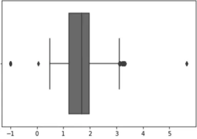
Venda Valor Unitário Médio

Regarding the variable that reflects the average price per unit of product sold, I noticed that although this value ranges between 1 and 2 in more than 50% of the observations, in some cases it assumes values superior to 3 or even below 0. Regarding the first case I didn’t consider it a problem since it is possible that some fruits have a price per unit of measurement higher than 3€, but regarding the second ones I will analyse it afterwards since in my perspective it might represent an incoherence.

Figure 3.1: Boxplot of the Venda Valor Unitário Médio variable

Venda Valor PC

As expected, the Venda Valor PC histogram shape is close to the one of the Venda Quantidade variable and especially to the one of the Venda Valor PV variable, they are highly related. Therefore, by

17 observing the histogram I could conclude that the big majority of values ranges between 0€ and less than 200€, even though the minimum value for this variable being less than -2€ and its maximum value being higher than 580€. Additionally, it is relevant to point out that this variable’s similar behaviour to

Venda Valor PV from the fact that the first represents the value of products sold without inclusion of

the profit (using the cost price of a product to calculate this variable) while the second one reflects the value of products sold with the profit (using the sale price of a product to obtain this variable).

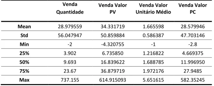
Venda Quantidade Venda Valor PV Venda Valor Unitário Médio Venda Valor PC Mean 28.979559 34.331719 1.665598 28.579946 Std 56.047947 50.859884 0.586387 47.703146 Min -2 -4.320755 -1 -2.8 25% 3.902 6.735850 1.216822 4.669375 50% 9.693 16.839622 1.688785 11.996950 75% 23.67 36.879719 1.972176 27.9485 Max 737.155 614.915093 5.651615 582.35245

Table 3.2: Summary of the statistical analysis of the four sales related variables

Stock Quantidade

According to the information previously obtained after applying the describe function, the amount of product available at a store varies from approximately -6894 to 1797 units of measurement, with more than 50% of the observations ranging between 19 and 90. An interesting conclusion that can be highlighted is that, as can be observed in the histogram, the range of negative values is wider than the range of positives, regarding the stock quantity of products.

Stock Valor

As expected, the histogram of the variable that reflects the value of the amount of product available at a store is very similar to the one that reflects the amount. The minimum of this variable is less than -13000€ and the maximum is higher than 1689€, with more than half of the observations assuming a value between 23€ and 107€.

Stock Cobertura

This variable is calculated using the variables that measure the stock quantity, the value of sales at a cost price and the number of days of each month. Although it ranges between approximately -1743 and 6142, more than 50% of its values are somewhere between 2 and 7, meaning that in over 50% of cases the product available in the store will last between 2 to 7 days, assuming the current usage continues.

18 Figure 3.2: Stock Cobertura formula

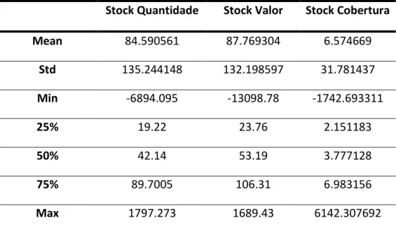
Stock Quantidade Stock Valor Stock Cobertura Mean 84.590561 87.769304 6.574669 Std 135.244148 132.198597 31.781437 Min -6894.095 -13098.78 -1742.693311 25% 19.22 23.76 2.151183 50% 42.14 53.19 3.777128 75% 89.7005 106.31 6.983156 Max 1797.273 1689.43 6142.307692

Table 3.3: Summary of the statistical analysis of the stock related variables

Quebra Identificada Quantidade

The variable that measures the quantity of identified losses assumes values between -278 and 90. Besides that, through the analysis of the histogram it is easy to understand that most values range between -50 and 50, with more precisely 50% of the values ranging between -2 and -0,25. At least 75% of the observations present a negative value (between -278 and -0,25) for this variable, meaning that at least three out of four observations represent an identified loss.

19 Figure 3.3: Sum of the quantity of identified losses, per month

Quebra Identificada Valor

Regarding the Quebra Identificada Valor variable, which measures the value originated by the quantity of identified losses, I can start by highlighting that it doesn’t assume negative values since it has a minimum value of 0. Additionally, 75% of its values range between 0 and 2,25, with the remaining 25% varying between 2,25 and 26 280, representing the most expensive and therefore most significant identified losses.

Quebra Inventario Quantidade

While analysing the variable that measures the quantity of unidentified or inventory losses, I concluded that, although it ranges between less than -444 and more than 294, only less than 25% of the observations are below 0, representing an unidentified loss. Moreover, less than 25% of the observations range between 0 and approximately 295, representing moments in which the inventory was measured and there was more quantity of a product in the store that it was expected. The remaining more than 50% observations have a value of 0 for this variable, meaning that probably in more than half of the observations the inventory wasn’t counted, which makes sense since it is supposed to be measures weekly.

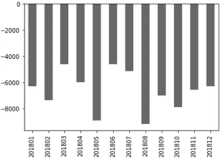
20 Figure 3.4: Sum of the quantity of unidentified losses, per month

Quebra Inventario Valor

The histogram of the Quebra Inventário Valor variable, as well as the information obtained from the use of the describe function, show that the value originated by unidentified losses ranges between 0 and aproximately 580, with at least 75% being equal to 0 and the remaining 25% assuming values between 0 and 579,6. Quebra Identificada Quantidade Quebra Identificada Valor Quebra Inventário Quantidade Quebra Inventário Valor Mean -1.976849 6.793631 -0.625015 2.9635 Std 4.910775 254.186453 11.274358 12.970371 Min -278 0 -444.71 0 25% -2 0.31 0 0 50% -0.92 1 0 0 75% -0.25 2.25 0 0 Max 90 26 280.79 294.99 579.6

21

3.2.2.2. Non-numerical data

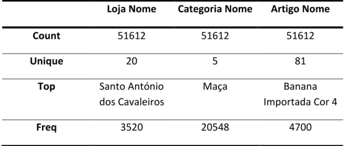
In order to assess the non-numerical variables, I applied the describe function, that returned the number of observations and the number of different categories for each variable, as well as the most observed category per variable together with its frequency (Table 3.5).

Loja Nome Categoria Nome Artigo Nome

Count 51612 51612 51612

Unique 20 5 81

Top Santo António dos Cavaleiros

Maça Banana

Importada Cor 4

Freq 3520 20548 4700

Table 3.5: Summary of the analysis of the non-numerical variables

Loja Nome

The provided dataset contains 20 different stores which were chosen by the company in order to reach all existent types of Pingo Doce stores. They were chosen among the more than 400 Pingo Doce stores existent in Portugal, in order to ensure that I would analyse a representative sample of all types of stores, both in terms of store size and location, as well as the usual quantity of customers.

Categoria Nome

By analysing the Categoria Nome histogram I concluded that the dataset has five different types of fruits, namely: citrinos, maça, uvas, pera and banana. The category with more observations is maça, with more than 20 000 observations, followed by citrinos with approximately 10 000 instances and uvas, pera and banana, with more than 5 000.

22

Artigo Nome

The provided dataset contains 81 different products, all distributed among the 5 categories. I analysed the number of observations per product name, obtaining the top 10 of the most observed products (Table 3.6).

Product Name Count of Observations

Banana Importada Cor 4 4700 Laranja Cal 3/4/5 3809

Uva Red Globe 2791

Limão Cal 3/4 2464

Maçã Royal Gala 70/75 2423 Pera Rocha 65/70 2315

Maçã Fuji 2194

Maçã Golden Alpes Itália 2124 Maçã Reineta Parda 75/80 1923

Uva Branca 1482

Table 3.6: Top 10 of the most mentioned articles

Ano

As expected, the variable that represents the year in which the transaction being analysed occurred only assumes one value, namely “2018”, since I only received data regarding the sales, stocks and losses movements that happened in the year of 2018.

Mês

By analysing the histogram of this variable, I could measure the number of observations that exist per month and conclude that December is the month in which more transactions occur, whether they are related to sales or losses measurements, followed by March and April. July was the month with less movements, followed by the remaining summer months (June, August and September).

23 Figure 3.6: Number of observations per month

Semana

The variable whose histogram reflects the transactions per week shows that it varies greatly depending on the time of the month and the time of the year. For instance, I can clearly notice a pattern in which approximately one week per month has a lot more observations than the three weeks that precede and succeed the referred week. Also, as in the month variable histogram, I can recognize a decrease in the number of movements in the summer months.

Figure 3.7: Number of observations per week

Data

The histogram of the Data variable reflects the movement of products, namely sales and losses, per day. Through its analysis I was able to identify at least eleven days in which the number of movements was much higher than usual, what might indicate the end of each month. I could also notice, as in the histograms related to the month and week, a decrease in the number of movements in the summer period.

24 Figure 3.8: Number of observations per day

3.3. D

P

After exploring all variables, data needs to be processed with the goal of converting it into high-quality data that will lead to the creation of high-quality models. Due to the existence of incomplete, noisy and incoherent data this is a fundamental stage of the Data Mining process, taking approximately 80% of the total process effort. Among the several possible tasks to perform in the data preparation phase, I performed the following: Data Import, Data Cleaning, Data Transformation and Data Reduction.

3.3.1. Data import

I started by importing the Excel file provided by the company to Spyder, since I am using Python 3.6.5 to develop this project. Using the pandas read_excel function I obtained a DataFrame with 51 612 rows, corresponding to the number of observations, and 21 columns, which corresponds to the number of features available.

3.3.2. Data cleaning

After importing the file and consequently creating the Dataframe, it is important to proceed to the Data Cleaning phase, that consists in a set of crucial steps such as removing duplicated observations and identifying and dealing with missing values, outliers and incoherent data, that will allow the algorithm created to have a better performance.

3.3.2.1. Removing duplicated observations

To remove any possible duplicated rows in the original dataset, although in a very broad look across the Excel file it didn’t seem that there would be any duplicated entries, I used the drop_duplicates function that returns only the dataframe’s unique values. After applying it, the DataFrame kept having the same number of rows, wherefore I could conclude that as expected there were no duplicated rows.

3.3.2.2. Missing values

In the Data Understanding chapter, more precisely in the Variable Analysis phase, I concluded that there were no missing values in any variable. To be sure of this assumption, I applied the isnull function,

25 that returns the number of null entries for each variable, allowing me to confirm that there are no missing values in any variable of the dataset. Therefore, I don’t need to make any changes to the original dataset.

3.3.2.3. Outliers

An outlier consists of an observation whose value is either much higher or much lower than most of the data, indicating that it may be some type of mistake. The big concern when dealing with outliers, is that, on one hand, altering them can lead to a better performance of the models, but on the other hand, they can be legitimate observations and sometimes the most relevant and interesting ones. That said, it is very important to understand the nature of an outlier before deciding how to act, once they shouldn’t be removed unless proven to be erroneous data.

I started by visually analysing the number of outliers in the original dataset but I found it a bad approach since, for instance, the quantity of sold products varies a lot between categories, namely products that belong to the Bananas category are sold a lot more than any product belonging to the Citrinos category. That said, I divided the original dataset into five different datasets, one per each category of product, namely: Banana, Citrinos, Maca, Pera and Uvas. First, I used the Z-Score method to identify outliers as observations that stand more than 3 standard deviations away from the mean of each variable. By using this approach, I obtained the following number of outliers, per category and per variable:

Banana Citrinos Maçã Pera Uvas Venda Quantidade 76 197 411 99 169 Venda Valor PV 76 207 387 88 148 Venda Valor PC 72 211 392 93 164 Venda VUM 2 31 181 60 29 Stock Quantidade 57 165 89 92 134 Stock Valor 18 156 99 88 154 Stock Cobertura 1 128 197 58 4 Quebra Identificada Quantidade 109 196 178 97 187

26 Quebra Identificada Valor 7 7 20 4 3 Quebra Inventário Quantidade 117 200 238 108 201 Quebra Inventário Valor 194 192 231 103 163

Table 3.7: Number of outliers using the Z-score method, grouped by variable and category of product After observing the results, I decided to take a closer look at the outliers, per variable, by analysing the respective boxplots, with the purpose of looking for the most significant outliers and also understanding which variables are most likely to contain wrong values, generated by human error, since I defined that only in that case an outlier should be removed. That said, I decided to remove outliers only on the two following variables:

1. Venda Valor Unitário Médio

I transformed the negative values, always equal to -1, to the median of the variable, per category, creating a new variable: Venda VUM.

2. Stock Quantidade

I consider this variable requires a lot of human input, what can cause several measure errors and, therefore, I decided to remove the most significant outliers. By observing the boxplot of this variable, I decided to replace its outliers with the median of the variable, also per category obviously, creating a new variable: Stock Qt.

Regarding to the outliers of the remaining variables, which didn’t suffer any change I can highlight a few reasons that led me to that decision, namely:

 Venda Quantidade

Initially I was determined to remove the outliers identified in the Citrinos, Maca and Uvas categories, due to their high number in comparison with Banana and Pera categories outliers. My idea was to remove any observation in which this variable assumed values higher than 300, 150 and 100, regarding the categories Citrinos, Maca and Uvas respectively, but after analysing the dates in which these observations occurred I concluded that the identified outliers correspond to Saturdays, Sundays or Tuesdays, which precisely correspond to weekends and to the first day of promotions of each week in the Pingo Doce stores. This led me to assume that probably the identified observations don’t correspond to errors but rather to correct values of sales on days in which customers are more likely to purchase these products.

 Venda Valor PV and Venda Valor PC

Since these variables are a product of the Venda Quantidade variable together with prices (PV and PC) that are automatically loaded into the company’s database, I found it hard to contain any wrong value.

 Quebra Identificada Quantidade, Quebra Identificada Valor, Quebra Inventário

27 Although these are the variables with the higher number of outliers, I decided to maintain all observations regarding these four variables, since they are the most relevant ones to this project and removing them might lead to loss of important information.

3.3.2.4. Coherence checking

While analysing the dataset looking for something that seemed illogical, I found several possible incoherencies among the data provided, namely:

1. Venda Valor PC > Venda Valor PV

I created a flag variable that assumes a value of 1 if the value of the variable Venda Valor PC is higher than the one of the Venda Valor PV variable, what means that the cost price of certain product was higher than the price it was being sold to the customers. I concluded that there are 1 759 observations in which this condition is observed. Although this might seem illogical, I didn’t consider it an incoherence since when a product is on sale it might be sold below its cost price. That said, I decided to maintain those 1 759 observations.

2. Stock Cobertura and Stock Qt have different signals

I created another flag variable that has a value of 1 if the variables Stock Qt and Stock Cobertura have different signals, being one positive and the other negative. This repreents an incoherence since logically, if the quantity of stock is positive then its coverage would still be positive and analogously, if the first is negative then the second should be negative. After analysing the flag variable created, I identified 158 observations in this situation. To understand this, I analysed the Stock Cobertura formula, that relates the Stock Qt variable with the Venda Valor PC variable and concluded that this happens when the second variable (Venda Valor PC) assumes negative values or is equal to zero. Since it is not possible to divide by 0, the company decided that when Venda Valor PC is equal to zero, the

Stock Cobertura variable takes automatically the value of -1. Therefore, since this was the best way

found by the company to deal with this situation, I decided to maintain these observations, not considering it an incoherence.

3. Venda Quantidade <= 0

The third flag variable I created has the objective of identifying the observations in which the variable

Venda Quantidade assumes non positive values. I considered this an incoherence since from my

perspective the company can only sell positive quantities of products. After analysing the flag variable, I concluded that there are 275 observations in which this happens. There are 9 observations in which the quantity of product sold is negative and 266 in which it is equal to zero. By performing a deep analysis of the dataset, I understood that in all observations with zero quantity of product sold, at least one of the variables regarding the identified or unidentified loss quantity is filled with a value different than zero. That said, I concluded that these observations, although not representing any sales information, are representing a moment in which the losses (identified or not) were measured. Therefore, I decided to maintain the 266 observations with value equal to zero. Regarding the 9 observations with negative values, I considered it an incoherence and since all those values range between 0 and -2, being little significant, I decided to change the negative values to zero, creating a new variable Venda Qt, that will be used instead of the Venda Quantidade variable from now on.