NON-PROPORTIONALITY IN RATIOS:
AN ALTERNATIVE APPROACH
DUARTE TRIGUEIROS
ISCTE, University of Lisbon
This study identifies general postulates underlying the validity of the financial ratio measurement. Then, new relationships are suggested obeying the same postulates, which may replace the ratio form in the case of non-proportionality. Where pro-portionality holds, these relationships revert to the traditional ratio. The paper also reviews the reasons for expecting non-proportional components in ratios and presents application examples of the new relationships. 1997 Academic Press Limited
INTRODUCTION
It is generally assumed that ratios remove the influence of firm size from corporate financial indicators. However, the widespread use of ratios in fin-ancial statement analysis has been criticized frequently in the accounting literature. Lev & Sunder (1979) and Whittington (1980) argue that size is only properly removed when the numerator and the denominator of the ratio are proportional. These authors advocate a regression rather than a ratio approach in order to remove size. Barnes (1982, 1986) and others reinforce these views. Horrigan (1983) and McDonald & Morris (1984, 1985, 1986) dissent, arguing that proportionality in ratios is irrelevant in judging their usefulness. This debate is summarized by Berry & Nix (1991).
Evidence on non-proportionality in UK industries is provided by Su-darsanam & Taffler (1995). McLeay & Fieldsend (1987) and Fieldsend et al. (1987) study proportionality in ratios in the presence of sector and size effects, showing that departures from proportionality may be accounted for, to some extent, by the interaction between these effects. Tippett (1990) shows that plausibly generated ratio components lead to inherently non-proportional ratios.
Only after understanding the reasons for the use of financial ratios can the above-mentioned limitations be put into a proper perspective. Indeed, given
Correspondence should be addressed to: D. Trigueiros, ISCTE, University of Lisbon, Avenida das Forc¸as Armadas, 1600 Lisbon, Portugal.
I would like to acknowledge the valuable contribution of Professor Stuart McLeay. Received 23 November 1995; revised 27 February 1996; accepted 1 July 1996
the peculiar characteristics of financial ratio components, any alternative form of financial indicator which is constructed from such variables ought to be selected with great care. Accordingly, this study first examines some general postulates underlying valid ratio analysis, and then considers the reasons for expecting non-proportional components in ratios. Based on such postulates, new relationships are suggested which may replace the ratio form in the case of non-proportionality. Where proportionality holds, these relationships revert to the traditional ratio.
GENERAL POSTULATES OF RATIO ANALYSIS
In essence, ratios compare two observations, yielding the proportion by which one differs from the other. However, ratios are not the most straightforward way of comparing observations. In many decision processes, the difference between two variables could be, and often is, used to the same effect. Why, then, are ratios required in the case of financial measurements? The reason is that, besides the interest in expressing results as proportions, the ratio form is also required for removing multiplicative statistical influences1 from
meas-urements. To be more precise, ratios provide the appropriate method of con-trolling for firm size if it is present in ratio components in the form of a multiplicative influence.
In fact, size is not removed by ratios when an additive influence is assumed. For instance, where two observations, y and x, are under the same additive statistical influence A (an expected value), then y and x are described as
y=A+ey
(1)
x=A+ex
eyand exbeing residuals (i.e. random amounts of y and x unexplained by A). In order to remove the influence of A, y and x should be subtracted. If, instead of subtracting them, a ratio were formed, then A would not be removed:
y−x=ey−ex whereas
y
x=
A+ey
A+ex
(2)
On the other hand, size is removed by the ratio when a multiplicative influence is assumed.2For instance, where two observations, y and x, are influenced by
the same S (an expected proportion), then y and x are described as
y=Sfy
(3)
fyand fxbeing random proportions of S found in y and x. In order to remove
S, a ratio of y and x, not a subtraction, should be formed:
y−x=S( fy−fx) whereas y x= fy fx (4)
However, not all types of multiplicative influence are removed by ratios. Ac-cording to the Law of Proportionate Effect,3each realization of a multiplicative
variable v is the outcome of many accruals dv, each of them proportional, on average, to values of v already attained. Therefore, in this case, the statistical influence commanding the generation of v is described by the percentage growth rate
ds=dv
v (5)
(which is independent of v), not by the accrual dv. Ratios of such variables may fail to remove size, because differences in their growth rates caused by stochastic fluctuations may generate co-variance terms which, in turn, in-troduce non-proportionality in the ratio form (Tippett, 1990). The adequacy of ratios also requires that any such distortion be negligible, but this will happen only if observations are generated by nearly constant, similar ds.
In summary, two general postulates underpin the validity of the traditional ratio measurement, which may be described systematically as follows. Given accounting variables y and x, which are assumed to be strictly proportional, with size present in the form of statistical influences dsxand dsy, and which are generated according to (5), then the ratio
y
x=Pfy/x (6)
will remove size (so that P, an expected proportion between y and x and firm-specific residuals fy/x, are independent of y and x) if:
(a) during the generation of individual observations the influence of firm size is the same for both components of the ratio (dsx=dsy, i.e. although case-related, ds is variable-independent); and
(b) such common influence is approximately constant.4
The first of these postulates, that of similar ds, underlies (3) and the simplified reasoning presented therein. It may be assumed that, when ratio components are taken from the same financial statement, they are generated under the same size influence. Indeed, the widespread lognormality of accounting variables (Trigueiros, 1995) suggests that the mechanism governing their distribution
is general rather than particular to different financial statement items. Thus, we may accept that, for ratios of items from the same financial statement,
dsx=dsy.
On the other hand, size will not be removed from the measurement when ratio components are generated under two different influences. This may be the case of ratios such as Return on Equity (ROE) or Return on Investment (ROI), for which it is frequent to take the denominator from the previous year’s report. Whereas, in the above ratios, the influence of size may be desirable (e.g. when measuring growth), other cases exist where such influence will be spurious. Earnings per Share (EPS) or Price/Earnings (PE) ratios, for example, may be correlated with size, because the statistical influence explaining the number of shares in issue is not necessarily the same as that commanding the generation of earnings.
The second postulate, that of constant ds, is a consequence of ratios having one degree of freedom only, enabling them to model just the expected value of growth rates, not their spread or their interaction. Constant ds implies that
v, in (5), grows according to a process of compounding (exponential growth).
If, however, the growth rate of firms varies widely, co-variance terms between ratio components may become significant. Seasonality, for instance, is sup-posed to undermine the accuracy of the financial measurement when the final value of a component fails to reflect its real growth during the period. However, according to this postulate, even in cases where it makes sense to assume that the magnitude of a ratio component reflects the way its growth has taken place, seasonality or any significant fluctuation might still distort the ratio measurement.
THE THRESHOLD RATIO
It may be asked whether it is possible to overcome some of the limitations of ratios without departing from the two conditions for valid ratio measurement outlined above. The Law of Proportionate Effect, for instance, acknowledges that the accrual dv in (5) may be proportional, not to v itself, but to v−d where d is constant. In this case
ds= dv
v−d (7)
instead of (5). Conditions leading to lognormal v in (5) generate, in (7), distributions known as three-parametric lognormal with thresholdd (Aitch-ison & Brown, 1957).
Three-parametric lognormality in accounting variables was reported in Tri-gueiros (1995) and shown to be a plausible source of non-proportionality in
Value 0
Probability density
Three-parametric
Two-parametric
Figure 1. The usual, two-parametric, lognormal distribution (solid line) and the corresponding three-parametric distribution (dashed line) showing a positive displacement, d, known as the threshold.
financial ratios, consisting of a displacement of the distribution of individual components (Figure 1). The existence of fixed costs, for instance, leads to a constant displacement in the distribution of total costs.
Adequate removal of size requires, in this case, one of the following ratios:
y−dy
x =Pfy/x (8)
y x−dx
=Pfy/x (9)
for, respectively, three-parametric lognormal numerators and denominators. Thresholds aredyin (8) anddxin (9). The above ‘threshold ratios’ cope with an elementary form of non-proportionality, albeit obeying the same postulates as traditional ratios. Where proportionality holds, thend=0 and they revert to the traditional ratio. If thresholds in the numerator and in the denominator are both significant, a reinforcement of non-proportionality occurs whendy anddxhave different signs. In a singular case, P=dy/dx, thresholds are cancelled out (functionally) but they still distort the analysis.
In addition to thresholds which are identical for a group of observations, it may also be worth considering size-related thresholds. In this case,d is similar to other accounting variables. Realizations of v will be larger than expected for comparatively larged (e.g. in cross-section, the case of large firms), and the growth rate ds is no longer variable-independent. A simplified view of
processes which assume size-related thresholds might be given by
dsv=bvds with ds=
dv
v and bv=f(d, v) so that bv→1 for d→0 (10)
Sinced is small for small ds and large for large ds, strictly size-related thresholds cannot generate non-proportionality between components. Assuming, for instance, thatb, an expected b for all realizations of v, exists, ratios based on (10) may take the form
y
xb=Pfy/x (11)
or similar. On a logarithmic scale,
log y−b log x=l+ey/x (12)
(12) is functionally identical to the relationship used by Fieldsend et al. (1987) for studying sector effects. It is a regression rather than a threshold ratio. The slope coefficient, b, is approximate to the unit in the case of strict pro-portionality. Slopes smaller than 1 are obtained ford<0. In cross-section, they bias a large firm’s ratios downwards, mimicking scale effects such as those described by Whittington (1980).
In practice, the same accounting variable may have both constant (size-independent) and size-related thresholds. In a time-series, for example, some fixed costs will generate constant thresholds, whereas others, which may follow a step function, will be sensitive to changes in size.
THRESHOLD RATIOS VS REGRESSIONS
Previous studies concerning the validity of ratios stress the fact that regressions may add to financial measurement the possibility of modelling non-pro-portional relationships. However, regressions add more than just intercept terms: they also introduce, through the slope coefficient, an estimation of correlation between components. Such estimation, not present in trad-itional ratio analysis, substantially changes the nature and scope of financial measurement.
Since ratios are simple proportions, the estimation of ratio benchmarks such as industry norms only requires the estimation of the expected values of components. In contrast, in a regression, both the slope and the intercept term
Denominator Numerator 4 6 4 2 2 6 0 (a) 4 6 4 2 2 6 0 (b)
Figure 2. The two variables (called numerator and denominator), displayed on the left and on the right, have the same expected values. Only the correlation between them is different and so, therefore, are the regression coefficients. (a) Correlation=0·7; E (ratio)=1; in-tercept=1·6; slope=0·6. (b) Correlation=0·9; E (ratio)=1; intercept=0·4; slope=0·9.
are influenced by the variance and co-variance of components (Figure 2). The improvement offered by threshold ratios (8) and (9) over traditional analysis is the possibility of modelling expected proportions irrespective of correlation, thereby preserving the ratio’s characteristics, which appear to be important to financial decision makers.
In the threshold ratio, for instance, non-proportionality is modelled as a constant displacement in the distribution of one of the components, whereas the regression intercept term stems from the interaction between the two variables. Only when the relationship between components is deterministic (i.e. correlation is equal to 1) are the regression coefficients readily in-terpretable in the same way as the usual ratio measurement.5
Functionally, ratio (9) is also different from regression in that its ‘intercept term’−dxP fy/x, is not constant. It depends not only ondxand P, but also on the residual fy/xin each case. The threshold in ratio (8),dy, might be viewed as similar to a regression intercept as it introduces a case-independent constant term. However, ratios (8) and (9) are essentially similar. On a logarithmic scale, they become, in the same order,
log( y−dy)−log x=l+ey/x (13)
log y−log(x−dx)=l+ey/x (14)
withl=log P and ey/x=log fy/x. On this scale, corrections introduced by a sim-ilar d in numerators or in denominators have the same magnitude. On the
original scale, denominators correct for distortions limited by the range {0, 1}, whereas numerators correct for magnified distortions that are greater than 1. The basic difference remains that the estimation of threshold ratio parameters does not require consideration of the variance and co-variance of components.
There are two other differences between threshold ratios and regressions. First, like traditional ratios, threshold ratios may be treated as errors-in-vari-ables models, where appropriate. In contrast, regressions require the as-sumption that independent variables are deterministic, yet, as Horrigan (1983) pointed out, ‘neither component [in ratios] is the exogenous, causal variable, nor is one component necessarily stochastic while the other is de-terministic’. Second, threshold ratios are consistent with the multiplicative character of the components, whereas the assumption underlying regressions is that variables are additive.
REASONS FOR EXPECTING NON-PROPORTIONALITY A distinctive characteristic of multiplicative variables is that, when a ratio is formed, the distortion introduced into the analysis by thresholds is likely to be negligible in most instances. That is, owing to their exponential growth, realizations of v in (7) may attain values many times larger than the threshold and, in such cases, v−d≈v. Non-proportionality is significant only where generative processes lead to realizations of v which are not much larger than d as, for example, in the case of a small growth rate ds.
As a consequence, comparatively large size-independent thresholds are plausible in time-series analysis, but unlikely in cross-section analysis. Ob-servations in a time-series have their origin in the same object (e.g. one firm or aggregate in different periods). Features which are constant inside firms, such as fixed costs, emerge as size-independent in this context, being able to create comparatively large thresholds. In cross-section, as observations have their origin in different objects, size-independence requires industry-wide ‘fixed costs’. Since these thresholds must allow for the survival of small firms, they must be comparatively small.6Therefore, where ratios are used for
norm-ative purposes, corrections of distortions caused by non-proportionality are likely to be required only when assessing deviations of small firms from industry norms. On the other hand, a pervasive, significant distortion caused by a threshold is possible only in industries where firms have similar sizes.
The existence of fixed costs is also likely to generate size-related thresholds [i.e. costs which are fixed for one firm but variable across firms, large firms having large fixed costs and small firms having small fixed costs (Lev & Sunder, 1979; Whittington, 1980) ]. In this case, the use of ‘slope ratios’ such as (12) may be appropriate.
In a time-series analysis, size-related thresholds are worth considering only where large changes in size have taken place. This will not normally occur
TABLE 1
Plausibility and effectiveness of thresholds in creating non-proportionality
Thresholds Analysis Constant (size-independent) Size-related
Cross-section Plausible only if small. Effective in Plausible but not effective. May distorting deviations of small firms cause false scale effects. from industry norms.
Time-series Plausible: any constant value inside Plausible but dominated by size-firms. Effective. independent thresholds.
when analysing a short period of time, where size-independent thresholds dominate the analysis.
Table 1 summarizes this discussion.
APPLICATION EXAMPLES
This section suggests methods for estimatingd and displays examples of the application of threshold ratios. The first example uses items Fixed Assets (FA) and Current Assets (CA) in a cross-section analysis.7The data set (Electronics
industry, 1986, UK firms only) is taken from the Micro-EXSTAT database. Five models are compared below.
Model 1: The Traditional Ratio
This model has one degree of freedom, the median of the ratio (l on a log-arithmic scale):
FA CA=10
lf or log FA=l+log CA+e (15)
Model 2: The Slope Ratio
This model has two degrees of freedom: l and b, the slope. The estimated model, similar to (12), is
log FA=l+b log CA+e corresponding to the ratio FA CAb=10
lf (16)
Graphically, this model is a straight line on a logarithmic scale and non-linear on an ordinary scale.
Model 3: The Threshold Ratio with Jointly Estimated Parameters
The two degrees of freedom of this model correspond tol and d. Those are estimated using
log FA=l+log(CA−d)+e corresponding to the ratio FA
CA−d=10
lf (17)
Graphically, this model is non-linear on a logarithmic scale and a straight line on an ordinary scale.
Model 4: The Threshold Ratio with Independently Estimated Parameters
In this model there is only one degree of freedom,l. d, the threshold of the distribution of CA, is known in advance.l is estimated using
log FA=l+log(CA−d)+e corresponding to FA
CA−d=10lf (18) Graphically, this model is non-linear and parallel with Model 3 on a log-arithmic scale and a straight line on an ordinary scale. The model converges with Model 1, the traditional ratio, for medium-sized and large firms.
Model 5: The Threshold Ratio Plus Slope
This model has three degrees of freedom,l, b and d, jointly estimated using
log FA=l+b log(CA−d)+e corresponding to FA
(CA−d)b=10
lf (19)
Graphically, this model exhibits a mixture of the features of Models 2 and 3.
Above, each model has been presented together with its logarithmic coun-terpart, as multiplicative models require logarithmic scaling prior to coefficient
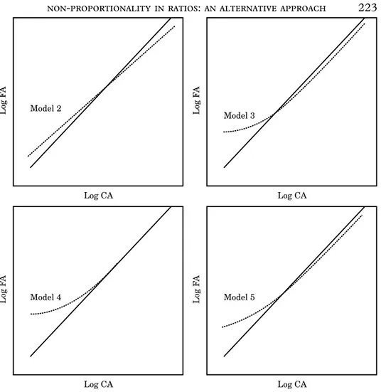
Model 4 Log CA Log F A Model 5 Log CA Log F A Model 2 Log CA Log F A Model 3 Log CA Log F A
Figure 3. The traditional ratio (solid line) when compared, on a logarithmic scale, with the slope ratio (Model 2), the threshold ratio (Models 3 and 4), and the threshold plus slope ratio (Model 5).
estimation. Figure 3 compares, on a logarithmic scale, Model 1 (solid line) with Models 2–5. Figure 4 reproduces Figure 3 on the original scale (only the region near the origin).
The independent estimation of thresholds, as in Model 4, can be carried out using any technique available to detect three-parametric lognormality in distributions. In this example we measureddCA=−£320,000, using a modi-fied version of the procedure suggested by Royston (1982, p. 123).8The joint
estimation ofd and other parameters, as in Models 3 and 5, requires iterative least-squares algorithms and logarithm-scaled models. Each of these methods
Model 4 CA FA Model 5 CA FA Model 2 CA FA Model 3 CA FA
Figure 4. The traditional ratio (solid line) when compared, on the original scale, with the slope ratio (Model 2), the threshold ratio (Models 3 and 4), and the threshold plus slope ratio (Model 5).
leads to a different interpretation of ratios and, in general, the estimates ob-tained also differ.
Table 2 relatesd and l obtained in each model to R2(variability explained),
skewness and kurtosis of e (residuals on a logarithmic scale). As can be seen, by letting the slopeb vary freely (Model 2), the R2approaches the variability
explained by thresholds (Models 3 and 4). Figure 3 also suggests that the slope approaches the effect of the threshold. Moreover, once d is accounted for, b returns to 1 (Model 5). Fieldsend et al. (1987) notice that slopes also tend towards the unit when sector effects are accounted for.
TABLE 2
Parameters and statistics obtained with the five models of the first example
Model No. l b d R2 Skewness Kurtosis
1 −0·46 72% 0·27 2·18
2 −0·21 0·94 76% 0·07 1·30
3 −0·49 −£528,000 78% −0·12 1·19
4 −0·46 −£320,000 76% −0·12 1·78
5 −0·40 0·99 −£403,000 78% −0·12 1·19
From the five models studied, the most attractive seems to be the threshold ratio where d and l are independently estimated (Model 4), as non-pro-portional components are accounted for, albeit also converging with the tra-ditional ratio for medium- and large-sized firms. Furthermore, the introduction in this model of one extra parameter,d,isnot likelyto significantly erode one of the strengths of the traditional ratio, robustness to irregular data, as the estimation of thresholds is exposed to ill influences only for a small portion of the sample.9This contrasts with the widened potential for distortion
introduced in estimates by slope coefficients.
When applying the traditional regression model (CA=a+bFA+e) to the same data set, some highly influential cases were observed using the procedure specified by Cook (1977). The intercept term, a, became much smaller and non-significant after removing the largest firm from the analysis. Weighted regression did not solve the problem completely, merely transferring the in-fluence from the largest to the smallest firms.10 Indeed, when included in
additive formulations such as regressions, multiplicative variables lead to es-timated coefficients which may be dominated by one or two influential ob-servations (Snedecor & Cochran, 1965, p. 290).
The second example illustrates an application of the threshold ratio method to time-series analysis, where Operating Costs and Sales of a UK retail firm (TESCO PLC) are examined for the period 1983–1987, following Steele (1989), i.e.: Year 1983 1984 1985 1986 1987 Operating £2,211m £2,518m £2,911m £3,216m £3,407m costs Sales £2,276m £2,594m £3,000m £3,355m £3,593m Ratio 97·15% 97·07% 97·03% 95·85% 94·84%
Typically, a regression where Sales is explained by Operating Costs would be expected to yield an intercept term which approaches fixed costs for that
TABLE 3
Comparing a regression with the threshold ratio in estimating fixed costs
Results
TESCO PLC 1983–1987 Regression Threshold ratio
Model used for estimating Costs=a+b Sales+e log Sales=
coefficients: l+log(Costs−d)+e
Estimated coefficients: a=£149m, b=0·91 l=0·036, d=£125m
(R2=99%) (R2=99%)
Functional form obtained: Costs−£149m Sales =0·91
Costs−£125m Sales =0·92
period. Table 3 shows the functional relationships used for estimation, and the results obtained when comparing the regression method with the threshold ratio method.
The relationship is, in this case, almost deterministic (R2=99%). As a
consequence, the slope of the estimated regression, b, is similar to the expected proportion, 10l, observed between the numerator and the denominator of the ratio. Should the correlation between sales and costs be smaller than 1 (while considering the same expected proportion), then b would be smaller than 10l. In the limit, for a correlation approaching zero, b would also become zero and
a would equal the expected value of the numerator. The expected ratio, 10l, would not change. This reasoning illustrates clearly the above-mentioned differences between threshold ratios and regressions, showing that, similarly to the traditional ratio, the threshold ratio explains costs as a proportion of sales irrespective of correlation. In addition, in the threshold ratio, fixed costs are explained as a constant displacement in the distribution of costs.
Fixed costs (costs incurred which do not change with the amount of product made) may, nevertheless, vary over time because of growth effects or changes in money values. Both methods assume that fixed costs are stable. However, when fixed costs are estimated as a displacement in the distribution of costs, the accuracy of the estimation is undermined by fluctuations in fixed costs only, whereas the estimation based on an intercept term is affected by fluctuations in fixed costs, by fluctuations in the slope coefficient (e.g. changes in efficiency or in sales prices) and by the interaction between these effects.
DISCUSSION
The literature on the validity of ratios to date has uncovered two cases where ratios may fail to remove size. First, components may be non-proportional (Lev & Sunder, 1979; Whittington, 1980 and others). Second,
even where components are proportional, co-variance between them in-troduces non-proportionality in the ratio form (Tippett, 1990). Practitioners, however, albeit acting guardedly in cases where financial ratios also have the potential to bias the analysis, such as the existence of seasonality, seem little concerned with non-proportionality. Indeed, empirical tests carried out so far, though finding clear traces of non-proportionality in ratios, do not support the view that such distortion is overwhelming. It seems as though non-proportionality has, in practice, little impact on the use of financial ratios. A few authors go as far as to argue that the issue may be irrelevant (Horrigan, 1983; McDonald & Morris, 1984).
This study has offered an alternative approach to the problem of non-proportionality in financial analysis which, amongst other practical con-sequences, explains the apparent contradiction outlined above. First, the paper suggested that the ability of financial ratios to remove size stems from firm size being present in both ratio components in the form of the same multiplicative statistical influence. In addition, distortion introduced in the measurement by co-variance terms is likely to be negligible where, during the generation of components, the influence of size can be taken as nearly constant.
In contrast with the usual statement that ratios are valid where pro-portionality holds, the above two postulates provide a basis for discussing the adequacy of ratios to specific tasks and, where necessary, for implementing improvements consistent with financial decision-making. The paper has explored the most obvious of such improvements. Since size is present in accounting variables in the form of a statistical influence, the removal of size only requires the modelling of proportionality between statistical influences. The condition of strict proportionality between components is, therefore, restrictive in excess. Earlier, it has been shown that, besides traditional ratios, other similar relationships exist which are capable of removing size, specifically the threshold ratio.
The above two postulates also help to put into perspective the limitations and strengths of traditional ratios, especially when compared with those of alternative tools. Limitations, for instance, stem from simplicity: any model with only one degree of freedom would display similar limitations, and it is easy to overcome those just by incorporating more degrees of freedom into models. However, the more degrees of freedom models have, the less intuitive the financial measurement will be, becoming sensitive to irregular data or influenced by conditions, such as the variance and co-variance of components, not necessarily required in the financial decision process.
The postulates also clarify circumstances in which non-proportionality may be effective in distorting the analysis. Given the exponential generation of accounting variables, reasons invoked for expecting significant distortions apply to time-series analysis, but are less plausible in cross-section. In the latter, only small firms are affected. Threshold ratios may provide, in these cases, more accurate analysis and statistical manipulation of data.
Finally, the fact that the additive formulation
y
x=A+e (20)
has been used routinely to discuss the validity of ratios and their statistical characteristics, may account for some of the recent academic criticism of the ratio method. Given the imposing a priori assumptions of the additive model, it is not surprising that ratios seem not to be up to the task.11It may
also be speculated that the adoption of relationship (20) was influential in viewing ratios as zero-intercept regressions (thence the interest in adding the missing term), rather than as simple proportions. In addition to calling attention to the initial judgement implied by (20) and to the contradiction it entails, the paper has suggested a more reasonable alternative, the mul-tiplicative form, in the light of which ratios agree with the statistical characteristics of accounting data.
N
1. For the sake of simplicity, the paper uses the term influence when referring to statistical effect. Multiplicative influences, known also as proportionate (or exponential) effects, are well documented in text-books in statistics. See, for example, Snedecor & Cochran (1965, 9th edition, p. 290). Lev & Sunder (1979) hint at the possibility of ratios being multiplicative models.
2. Authors tend to use additive forms such as (1), probably because these forms relate to the Normal distribution. However, evidence suggests that accounting variables are lognormal rather than normal, denoting multiplicative influences. Lognormality in variables such as Sales, Earnings and Total Assets, received a great deal of attention in texts on the theory of the growth of firms (e.g. Ijiri & Simon, 1977). In the accounting literature, McLeay (1986) mentions lognormality in variables which are sums of similar transactions with the same sign such as Stocks, Creditors or Current Assets. Recent empirical evidence (Trigueiros, 1995) suggests that lognormality is widespread. 3. The Law of Proportionate Effect is the mechanism explaining multiplicative influences.
See, for example, Gibrat (1931, pp. 62–64); Aitchison & Brown (1957, pp. 20–27). McLeay (1986) relates this mechanism to distributions found in ratio components. 4. The two postulates are not meant to offer insights into the characteristics of individual
financial statement items or particular ratios. Differences in expected magnitudes ob-served in accounting variables and random deviations from these magnitudes may have their origin in initial values (values of v at the beginning of the generating process) or other conditions which uniquely determine observations generated by (5).
5. In this case, the slope is the proportion between average numerator and denominator and the intercept term is their difference.
6. For example, an industry-wide average cost of £3,852,000 for food manufacturers in the UK in 1987 would represent only 0·2% of United Biscuits earnings, but it would equal the turnover of a small firm such as G. F. Lovell plc. The volume of sales of United Biscuits was, in 1987, about 480 times the volume of Lovell, a typically multiplicative proportion. Additive observations, such as the height of adults, do not exhibit such huge discrepancies.
7. These variables were chosen becausedFAis non-significant, and also because accounting identities cannot distort the distribution of their ratio (Trigueiros, 1995).
8. Royston uses trial and error to find out whichd maximizes W in the Shapiro & Wilk test of normality.d estimated by the Royston method is too large in most cases. To avoid overestimation,d should be estimated as the smallest d in z=log(v−d) able to render z=N(l, r).
9. Even so, some loss of robustness is expected when using threshold ratios. Three-parametric lognormality, for instance, might be less frequent than that suggested by statistical tests, as other anomalies impinging upon the smallest values in a distribution also benefit from the introduction of the three-parametric transformation in such tests. However, the fact that the industrial grouping mostly determines whether samples are expected to be non-proportional (McDonald & Morris, 1984; Fieldsend et al., 1986; McLeay & Fieldsend, 1987; Sudarsanam & Taffler, 1995; Trigueiros, 1995), gravitates against viewing thresholds purely as ‘catch-all’ terms.
10. Weighted regression stabilizes variance in proportion to the independent variable. In multiplicative data, variance is proportional to the square of the independent variable. Anyhow, the statistical characteristics of ratio components clearly suggest the use of multiplicative forms (or, for estimation purposes, their logarithmic counterparts), not weighted regressions. When these characteristics are overlooked, influential cases, not just heteroscedasticity, is what invalidates estimation. Therefore, the eventual robustness of estimation in the presence of heteroscedasticity (Barnes, 1986) is not, in this case, an important issue.
11. Tippett (1990, p. 80), in a time-series context, notices one example, amongst others, where (20) is contradictory: when e is large enough, then ratios may assume negative values, even where both components are, by definition, positive.
R
Aitchison, J. & Brown, J. (1957). The Lognormal Distribution, Cambridge University Press. Barnes, P. (1982). ‘Methodological implications of non-normally distributed financial ratios’,
Journal of Business Finance and Accounting, Vol. 9, No. 1, pp. 51–62.
Barnes, P. (1986). ‘The statistical validity of the ratio method in financial analysis: an empirical examination: a comment’, Journal of Business Finance and Accounting, Vol. 13, No. 4, pp. 627–635.
Berry, R. & Nix, S. (1991). ‘Regression analysis vs ratios in the cross-sectional analysis of financial statements’, Accounting and Business Research, Vol. 21, No. 82, pp. 107–117. Cook, R. (1977). ‘Detection of influential observations in regressions’, Technometrics, Vol.
19, pp. 15–18.
Fieldsend, S., Longford, N. & McLeay, S. (1987). ‘Industry effects and the proportionality assumption in ratio analysis: a variance–component analysis’, Journal of Business Finance
and Accounting, Vol. 14, No. 4, pp. 497–517.
Gibrat, R. (1931). Les Ine´galite´s E´ conomiques, Librairie du Recueil Sirey, Paris.
Horrigan, J. (1983). ‘Methodological implications of non-normally distributed financial ratios: a comment’, Journal of Business Finance and Accounting, Vol. 10, No. 4, pp. 683–668. Ijiri, Y. & Simon, H. (1977). Skewed Distributions and the Size of Business Firms,
North-Holland, Amsterdam.
Lev, B. & Sunder, S. (1979). ‘Methodological issues in the use of financial ratios’, Journal
of Accounting and Economics, December, pp. 187–210.
McDonald, B. & Morris, M. (1984). ‘The statistical validity of the ratio method in financial analysis: an empirical examination’, Journal of Business Finance and Accounting, Vol. 11, No. 1, pp. 89–97.
McDonald, B. & Morris, M. (1985). ‘The functional specification of financial ratios: an empirical examination’, Accounting and Business Research, Vol. 15, No. 59, pp. 223–228. McDonald, B. & Morris, M. (1986). ‘The statistical validity of the ratio method in financial
analysis: an empirical examination: a reply’, Journal of Business Finance and Accounting, Vol. 13, No. 4, pp. 633–635.
McLeay, S. (1986). ‘The ratio of means, the mean of ratios and other benchmarks’, Finance,
Journal of the French Finance Society, Vol. 7, No. 1, pp. 75–93.
McLeay, S. & Fieldsend, S. (1987). ‘Sector and size effects in ratio analysis: an indirect test of ratio proportionality’, Accounting and Business Research, Vol. 17, No. 66, pp. 133–140. Royston, J. (1982). ‘An extension of the Shapiro and Wilk’s test for normality to large
samples’, Applied Statistics, Vol. 31, No. 2, pp. 115–124.
Snedecor, G. & Cochran, W. (1965). Statistical Methods, Iowa State University Press. Steele, A. (1989). ‘The analysis of sales margins’, The Investment Analyst, Vol. 92, April, pp.
18–22.
Sudarsanam, P. & Taffler, R. (1995). ‘Financial ratio proportionality and inter-temporal stability: an empirical analysis’, Journal of Banking and Finance, Vol. 19, pp. 45–60. Tippett, M. (1990). ‘An induced theory of financial ratios’, Accounting and Business Research,
Vol. 21, No. 81, pp. 77–85.
Trigueiros, D. (1995). ‘Accounting identities and the distribution of ratios’, British Accounting
Review, Vol. 27, No. 2, pp. 109–126.
Whittington, G. (1980). ‘Some basic properties of accounting ratios’, Journal of Business