FUNDAÇÃO GETULIO VARGAS
ESCOLA de PÓS-GRADUAÇÃO em ECONOMIA
Raul Guarini Riva
Risk Prices and Model Selection: Bad
News About Sparse Estimators and an
Uniformly Valid Inference Theorem
Rio de Janeiro 2019
Raul Guarini Riva
Risk Prices and Model Selection: Bad
News About Sparse Estimators and an
Uniformly Valid Inference Theorem
Dissertação para obtenção do grau de mes-tre apresentada à Escola de Pós-Grauação em Economia
Área de concentração: Finanças
Orientadores: Caio Almeida e Yuri Sapo-rito
Rio de Janeiro 2019
Dados Internacionais de Catalogação na Publicação (CIP) Ficha catalográfica elaborada pelo Sistema de Bibliotecas/FGV
Riva, Raul Guarini
Risk prices and model selection : bad news about sparse estimators and an uniformly valid inference theorem / Raul Guarini Riva. – 2019.
44 f.
Dissertação (mestrado) - Fundação Getulio Vargas, Escola de Pós- Graduação em Economia.
Orientador: Caio Almeida . Coorientador: Yuri Saporito. Inclui bibliografia.
1. Modelo de precificação de ativos. 2. Risco (Economia). 3. Mercado Financeiro. I. Almeida, Caio Ibsen Rodrigues de. II. Saporito, Yuri Fahham. III. Fundação Getulio Vargas. Escola de Pós-Graduação em Economia. IV. Título.
CDD – 332.6
Risk Prices and Model Selection: Bad News About Sparse
Estimators and an Uniformly Valid Inference Theorem
Raul Guarini
Advisors: Caio Almeida and Yuri Saporito M.Sc. Final Paper - FGV/EPGE
May 24, 2019
Abstract
Lots of risk factors have been published in Finance papers in the last 20 years. Under a large menu, it’s hard to manually construct factor models with data-driven discipline and, more importantly, it’s difficult to assess the contribution of each newly proposed factor. We present some new literature on the usage of Machine Learning techniques to tackle this problem and discuss how to perform uniformly valid statistical inference on linear factor models for the stochastic discount factor. We provide further simulation evidence in favor of [Belloni and Chernozhukov, 2014] and discuss the method in [Feng et al., 2019] in detail.
1 Introduction
The question of what type of variables drive asset returns and how this kind of phenomenon takes place has been under modern discussion since the early days of [Markowitz, 1959] and [Sharpe, 1964]. Later on, the modern Macroeconomics literature started to embed this kind of discussion in the so-called “structural models”. Famous examples of such attempts are [Lucas, 1978], which became the workhorse of Economists to think about asset prices (and returns), and [Mehra and Prescott, 1985].
This kind of models relies on precise and abstract descriptions of the economy’s physical environment and try to obtain equilibrium results regarding endogenous variables such as consumption, savings and, in some incarnations, financial asset prices. The appeal of these models is twofold. First, they are useful story-telling devices that, when successful, match economic interpretation and optimal decisions by different agents. Second, writing structural models in Economics to study a given phenomenon is such a stringent requirement for the researcher that the train of thought guiding model design cannot be undisciplined. This implies, as an example, that these models are safeguards against spurious relations in econometric policy evaluations, as noted by [Lucas, 1976].
However, models are not useful only for understanding phenomena, but also to generate predictions. And, as an attempt to describe some sort of relation, the desirability of a given model is as strong as its
capacity to match real data and reproduce empirical regularities. As exposed by the famous example of [Mehra and Prescott, 1985] and highlighted by [Cochrane, 2005], the structural approach to explain or predict asset prices presents severe problems when confronted with data. This motivates the search for alternative techniques.
One possibility is a complete departure from this framework and the adoption of a purely statistical approach. The great disadvantage is losing the economic story-telling capability. A compromise solu-tion is to model features that appear endogenously in structural models with exogenous components. An example is to model the stochastic discount factor (SDF) with ad-hoc variables. Even though these variables might not arise in structural models as ones which are directly connected to SDF’s, they might be able to improve empirical performance in terms of forecasting or, even, in terms of explaining the cross-section of returns. Factor models are a by-product of this type of compromise solution. On a practical side, a quantitative finance practitioner might also be interested on factor models if they are really able to explain co-variation in returns. Factor models are useful tools for risk analysis, with diverse possible applications. Traders can use this type of models to hedge against several risk sources and, more broadly, have a better understanding of what type of shocks could impact asset returns and portfolio performance. General investors can assess the type of market risks they are exposed to when picking assets or even when choosing active managers for their funds. Also, high-frequency arbitrageurs can use factor models to exploit opportunities due to regimes of higher volatility since this type of model accounts for the interplay between the correlation of asset returns with the factors themselves.
From the 90’s on, the hunt for better factor models has been a great theme in the Financial Economics research agenda. Once we don’t expect theorists to come up with new possible factors and rely on data anomalies to propose new models, questions such as how to uncover true factors and how to estimate such models become top priority. Since the seminal work of [Fama and French, 1992] and [Fama and French, 1993], several new factors have been published in Finance papers, up to the point that it became very hard for a practitioner choose from a very long menu, as highlighted by [Harvey et al., 2016] and [Cochrane, 2011].
Recent developments on this field employ model selection techniques already studied by the Machine Learning community to pick factors in a data-driven way, such as the LASSO from [Tibshirani, 1996] and the Elastic Net from [Zou and Hastie, 2005]. The major drawback is that final estimators will, in general, be cursed by non-uniform approximations towards limit distributions. This implies that standard point-wise asymptotic theory can be misleading about inference on estimated parameters. Such behavior has also previously appeared in Econometrics in the theory of Instrumental Variables with weak instruments and in auto-regressive models with nearly integrated series. These Machine Learning estimators are non-uniform due to the fact that they are sparse, in the same spirit as the so-called Hodge’s Estimator, that is famous in the statistical literature for motivating the discussion around regular and non-regular estimators, as noted by [Bijma et al., 2016].
pricing information that is not spanned by previous factors. For doing so, the econometrician should estimate the risk price of a newly proposed factor, as noted by [Cochrane, 2005]. However, choosing the correct controls for a linear regression approach, for instance, is a daunting task for the same reasons as choosing which factors to include in a model in face of several options. Including too few controls can lead to omitted-variable bias. If too many are included, the model might overfit the data. Hence, model selection, estimation and inference should be conducted in a consistent way.
The work of [Belloni and Chernozhukov, 2013] and [Belloni and Chernozhukov, 2014] on treatment effects in high-dimensional designs was adapted by [Feng et al., 2019] for the linear factor model en-vironment, recovering uniformly valid asymptotic results. They provide statistical tools for testing if a newly proposed factor has a non-zero risk price after accounting for the effect of other factors, and such inference is uniformly valid. The next sections of this work briefly review the literature on factor models, present the model selection framework and its impossibility results regarding sparse estimators, provide further Monte Carlo simulations that strengthen the work of [Belloni and Chernozhukov, 2014] and detail the method from [Feng et al., 2019]. The final two sections offer ideas for future research and conclude.
2 Literature Review
2.1 Early Anomalies
Already in the late 80’s and early 90’s, there was compelling evidence that the so-called CAPM model of [Sharpe, 1964] had trouble to explain average returns using a market portfolio as a proxy for systematic risk. The usual approach at that time, which is still common in the applied literature, was to model the average returns directly. In this case, the expected return on a given stock is seen as a linear combination of the return on a risk-free asset and the return on the market portfolio:
E(Ri) = Rf+ βiE(Rm− Rf)
where Ri is the return on an asset i, Rf is the risk-free rate, Rm the return on a diversified market
portfolio and βi the coefficient measuring the exposure of asset i to the market factor, usually found
using a time-series regression of assets i’s excess return (its return minus the risk-free rate) on Rm−Rf.
By this model, the cross-section of expected returns should be explained solely by the exposure of a given asset to the market portfolio. With such a simple model, it’s not surprising that some empirical contradictions started to be found. As reviewed in [Fama and French, 1992], famous contradictions were:
• Size effect: the Market Equity (price of shares times shares outstanding) should add no relevant information in forecasting returns if the above model is correct. However, in the early 80’s, it was already stablished that small firms had returns well above what CAPM would predict. On the other hand, for big firms the opposite effect was detected on data.
• Leverage effect: another anomaly that would advocate against the previous model was a positive relation between leverage and higher returns. Although the argument that firms with higher leverage should have higher cost of capital (and higher returns in equilibrium) since they are riskier for the shareholders is in line with standard economic intuition, any kind of such relation had to be captured through equity βi on this model, and this was not the case.
• BE/ME effect: the ratio between book equity (defined as total assets minus liabilities) and market equity was found to help explaining returns, even after controlling for β’s. Again, any such relation should be captured by equity exposure to the market factor.
Actually, the main contribution of [Fama and French, 1992] was to discuss these empirical regularities and show, using the standard two-stage regressions method of [Fama and MacBeth, 1973], that easily measured variables as market equity (ME) and book-to-market ratio (BE/ME) could have explanatory power concerning asset returns. Market β’s could not account for all the cross-sectional variation of a selection of portfolio returns with different profiles of market equity and systematic risk exposure. That paper paved the road for future research in at least three important dimensions:
1. If one is concerned either with explanatory power of past returns or with forecasting performance of future returns, then the standard model should be augmented with new variables. As a first try, variables related to market equity and book-to-market ratio seemed the way to go. It’s not clear that this kind of variables carry pricing information per se, but they might be related to latent risk sources that are important for asset pricing but impossible to be measured by the researcher. In the end, the message was that we needed more factors.
2. There was no structural motivation on why, say, book-to-market ratio should be related to returns. One possibility for theoretical research would be trying to find a model based on agents and optimal choices that could support the use of such a variable. Another possibility, which can be seen as the winner route a couple decades after their seminal paper, was to relax the requirement of structurally-motivated variables to explain returns and experiment a little bit more with other ad-hoc variables. This, in a general framework, poses the question of how to identify and test factors.
3. Most financial ratios are scaled versions of other financial ratios. Hence, they may be correlated and this probably implies on the redundancy of some factors. If a number of financial ratios, or macroeconomic variables, are related to latent risk in the same manner, one should expect that adding all of them to an asset pricing model might improve results only marginally compared to the case in which only a few are added. Not all information is signal, financial data can be full of noise.
Their later paper, [Fama and French, 1993], proposed the so-called 3-factor model for stock market equity. They built two factors to explain equity returns (adding up to 3 when one considers the
traditional market return factor from CAPM). These factors were precisely engineered to capture the Size effect and the BE/ME effect.
They sorted stocks in different groups, using two independent metrics: market cap and BE/ME ratio. The factors proposed to explain stock returns were HML (short for High Minus Low, accounts for the BE/ME effect) and SMB (short for Small Minus Big, accounts for the size effect). These are returns on long-short portfolios constructed using the sorted stocks. In greater detail, the HML factor is the return of a portfolio long on firms with high BE/ME ratio and short on stocks with low BE/ME ratio. Similarly, SMB is return of a portfolio that is long on small stocks and short on stocks with high market cap. This methodology became the norm in Empirical Asset Pricing for constructing characteristic-based factors. They estimated the following model:
Ri,t− Rf,t= αi+ βi,M KT(RM,t− Rf,t) + βi,SM B· SMBt+ βi,HM L· HMLt+ εt
where the left-hand-side test assets were other sorted portfolios also constructed using the two afore-mentioned metrics but in much finer grids1.
A standard way of testing these models is to look for the R2 of these regressions as a measure of
explanatory power. Another way is to test if αi = 0. Because we are dealing with excess returns on the
left-hand-side and the right-hand-side has only excess returns or returns on zero-investment portfolios, αi should be zero for any asset or portfolio i due to rational expectations. After all, in this setting, αi
can be seen as a pricing error by economic agents, also called as “abnormal returns”.
Their main results were that the inclusion of these two factors was key to generate in-sample good performance of this model, at least for their data. Compared to the CAPM benchmarks, the inclusion of both factors shrunk α towards zero and improved the (adjusted) R2 metric by a large amount. This
methodology of creating long-short portfolios of stocks sorted according to some characteristic and using them as returns became the norm in empirical asset pricing after their earlier papers.
A possible criticism is that they were not challenging their factors enough. The main reason is that they were using other portfolios sorted qualitatively on the same way as their factors as test assets. Later empirical evidence exposed some more anomalies that advocate against CAPM and even against the 3-factor model. [Novy-Marx, 2013] identifies that a proxy for expected profitability is strongly correlated with average returns, for instance. If correct, the 3-factor model should account for this type of effect through the factors. [Aharoni et al., 2013] was able to expose a certain correlation between firms that make huge capital investments and firms that produce lower than expected returns, even after controlling for size and BE/ME ratio. As natural as it sounds, newer literature started to uncover anomalies on data that were not aligned with the 3-factor model, as in [HOU and ROBINSON, 2006] and [Heston and Sadka, 2008].
An augmented model, now with 5 factors, was proposed in [Fama and French, 2015]. The new factors tried to account for cross-sectional variation in returns due to different policies regarding investments
1We could, in principle, be interested in testing the model against the time series return of an individual stock but
any such model would probably have a poor performance since the amount of idiosyncratic risk that it would have to account for is probably large.
by firms and different past trajectories of profitability. These new factors were also constructed as returns on zero-investment portfolios. As expected, [Fama and French, 2015] could show that, while their 3-factor model struggled to explain returns of portfolios with varying degrees of profitability and investment profiles, the 5-factor model was able to handle these cases much better. Moreover, it had better performance than the 3-factor model in almost every test, both in terms of goodness of fit and small intercepts.
The fact that a 5-factor model outshines the 3-factor model should not be taken as a surprise. But if we are willing to accept new factors motivated solely on empirical regularities for the sake of empirical per-formance, why not a 6-factor model? Or a 20-factor model? There’s no clear limit. The risk embedded on asset returns is multidimensional and much of the decision process regarding optimal asset allocation by agents is not observable by the econometrician. It’s actually expected that several variables might prove useful to explain (and forecast) returns. For example, [Barrilas and Shanken, 2018] already ar-gue for a 7-factor asset pricing model and show that it consistently beats other famous models in the literature of asset pricing, including the one in [Fama and French, 2015]. How long will it take until we have a bigger model with more factors that beats the one proposed in [Barrilas and Shanken, 2018]? Not much if we consider the high number of available factors, as discussed in [Feng et al., 2019].
2.2 Model Selection
As hinted in the previous section, most of the traditional factor model literature for empirical asset pricing has been devoted to spot data anomalies that can generate factors, propose them and conduct tests. This type of research has brought us to the point that a “zoo” of possible factors exist, a term coined by [Feng et al., 2019]. From the econometrician’s point of view, the use of techniques designed for high-dimensional designs became more important. Choosing which factors to include in a model is, essentially, a problem of model selection. Thankfully, this has been well studied by the Statistics community. Standard updated references are [Bijma et al., 2016] and [van der Vaart, 2012].
In the late 90’s, [Tibshirani, 1996] proposed the LASSO (Least Absolute Shrinkage and Selection Operator) as a way to perform model selection in high-dimensional linear models through a L1-penalty
on parameters. This can also be seen as a constraint on the number of non-zero coefficients. Later, [Zou and Hastie, 2005] improved upon the LASSO with the Elastic Net techinique, which employs both L1and L2 penalties on parameters, of varying intensities. Interestingly, such estimators also have
Bayesian interpretations once Gaussian or Laplacian priors come into play. All these techniques (and several other ones) are covered in [Hastie et al., 2009].
In general, the estimators used in model selection techniques are designed for having maximum ef-ficiency in the task of deciding if some parameter is zero or not. The cost for that can be all sorts of non-uniformity and complicated asymptotic distributions, as seen in [Bickel et al., 2009], [Chatterjee and Lahiri, 2012], [Leeb and Pötscher, 2005], [Leeb and Pötscher, 2008] and [Pötscher, 2008]. The direct implication is that inference about estimated parameters is a fairly complicated matter.
Recently, [Belloni and Chernozhukov, 2013] showed a way to improve on the standard LASSO in terms of rate of convergence to the true parameter in L2-norm. Bounds on the LASSO’s rate of convergence
when penalty parameters are chosen by cross-validation were proved by [Chetverikov et al., 2019]. This is specially important in this context since cross-validation is a standard technique for choosing the LASSO (and Elastic Net) penalty.
Afterwards, [Belloni and Chernozhukov, 2014] proposed a method to recover uniformly valid results in a microeconometrics framework, tailored for applications in Industrial Organization and Labor Economics, for example. This is the method we provide further simulation evidence in favor of. A major deal of this theory on treatment effects in high-dimensional setups is reviewed in [Belloni et al., 2015].
2.3 Finance and Machine Learning
With data-driven selection methods such as the LASSO at hand, financial econometricians can now work with high-dimensional factor models. Another common technique from the Statistics/Machine Learning literature is the Principal Component Analysis (PCA), which is useful for dimensionality reduction. Sometimes, it’s easier to work directly with models for the SDF. This is only a choice of language since there’s a one-to-one correspondence between linear models for the SDF and linear factor models for returns, as in [Cochrane, 2005]. The link is done by the standard pricing equation
E(mtrt) = 1
that arises in structural models, where mtand rt represent the SDF and a given return, respectively.
More than that, linear factor models for the SDF are well grounded on theory, since [Hansen and Jagannathan, 1991]. They showed, using a good deal of functional analysis, how to construct a SDF that is linear on returns.
Such SDF always exist under mild assumptions regarding the stochastic processes driving returns. They also showed that, although sometimes it’s impossible to identify a unique SDF, all possible SDF’s are subject to some constraints regarding mean and variance.
As an example of research in the intersection of Finance and Machine Learning, [Kozak et al., 2018b] develop a methodology using regularization techniques and PCA to build and estimate a linear factor model for the SDF that achieves good out-of-sample performance in pricing assets. Their main con-tribution is showing how model selection can work in high-dimensional designs where several factors are available. The main challenge in such designs is not fitting noise while still uncovering the true factors from data that consistently produces small pricing errors out of sample. The Machine Learning literature uses the term robustness to refer to this type of desirable feature.
They also show how important is the choice of penalty parameters (two in the case of Elastic Net, only one if LASSO is used). Performance drastically changes as penalty parameters move. Nonetheless, they never show how smooth their SDF is, which can possibly make it not satisfy the bounds found by [Hansen and Jagannathan, 1991]. They do not worry about non-uniform estimators since they never perform proper inference on estimated risk-prices.
[Kelly et al., 2017] use PCA and their Instrumented PCA (IPCA) to recover factors from data, al-lowing latent factors that are instrumented by a given rotation of return data. They show that the tangency portfolio derived from the IPCA methodology achieves a higher Sharpe ratio than the one from [Fama and French, 2015]. They also show that only few characteristics truly help explaining their cross-section of returns even letting more than 30 to be chosen by IPCA. This result is in line with the findings from [Kozak et al., 2018a] and [Kozak et al., 2018b], who argue that sparsity in economic models can be recovered once we use Principal Components.
[Feng et al., 2019] adapt the post-selection estimator from [Belloni and Chernozhukov, 2014] in or-der to check if recent published factors after 2012 have non-zero risk prices after accounting for several previously published factors. They find that only some of them do. Actually, they advo-cate that if their methodology had been used extensively before, only some factors would have been published along the last decades. Importantly, results are drastically different if only the 3 factors from [Fama and French, 1993] are taken into account. They conclude that the most successful re-cent factors for American stock market data are the ones related to profitability. Arguably, how-ever, their main contribution is a methodological one, adapting the Double-Selection estimator from [Belloni and Chernozhukov, 2014].
Many of the recent developments in empirical asset pricing with Machine Learning are reviewed in [Kelly et al., 2018]. They compare different techniques that can be used in different scenarios in order to achieve better forecasting performance out of sample. Results argue in favor of simple regression trees and neural nets. These techniques, in special neural nets, are known to be useful in highly non-linear problems. Although [Hansen and Jagannathan, 1991] offered an initial theoretical starting point for using linear models, there is little beyond that to believe linear models are accurate in such complicated setups.
On Macrofinance, [Giannone et al., 2018] use LASSO-like estimators to advocate against the use of sparse models. Their main argument is that there is too much interplay between observable character-istics in Economics datasets, which in general make sparse models work poorly. We disagree regarding the definition of sparsity and discuss this claim in later sections. Exploiting the use of Machine Learn-ing as a numerical analysis tool, [Duarte, 2018] solves PDE’s that appear in Bellman problems from Finance and Macroeconomics. Although non-linearity makes closed-form solutions hard to obtain, he shows that these methods still work well in problems with a high number of state variables.
Regarding uniformly-valid results for linear factor models, [Bryzgalova, 2016] exposes the link between weak factors and weak instruments, known to cause problems in the microeconometrics literature. She also uses a LASSO-like estimator to perform model selection and guard against spurious factors. Although in a slightly different setup, it’s the closest paper to [Feng et al., 2019], to the best of our knowledge.
3 Model Setup
We describe the basic design from [Feng et al., 2019] and review the theory on sparse estimators on the next section. Following their notation, in order to develop a methodology to check if newly proposed factors really carry pricing information, i.e., have non-zero risk prices truly driving returns, consider a linear factor model for the Stochastic Discount Factor (SDF):
mt= 1/γ0
!
1− λ⊺ggt− λ⊺hht
"
(1) where γ0 is a zero-beta rate, gt is a d-dimensional column vector of factors to be tested and ht is a
p-dimensional column vector of factors that can be used as controls. Both gt and ht are de-meaned.
The goal is to perform inference on λg, the risk prices of newly proposed factors. This parameter
reveals whether gt drives returns by affecting the stochastic discount factor after accounting for the
effect of ht. In addition, it also reveals how gt affects mt. For example, a positive λg shows that an
increase in gt lowers the stochastic discount factor, hinting at low-marginal-utility states if one has
a structural framework in mind. The whole methodology is agnostic regarding the nature of these (potentially) new factors: it does not matter if they are motivated by economic theory or data mining. The naive procedure would be including lots of already studied factors in ht and run OLS. This is not
adequate since such simple method would probably overfit data (or fit noise, as is the standard language in Financial Econometrics). Moreover, the practitioner could end up with a model that is larger than necessary, which is harder to estimate, due to possible redundancy between factors. Additionally, we would like to have the freedom to work in environments in which truly large models are possible and we have more potentially important controls than data points. Then OLS becomes infeasible2 and we
need a new method anyway.
Notwithstanding, if the practitioner manually picks a couple factors for htfor the sake of keeping the
model small, she can be hunted by the classic omitted-variable bias. Model selection techniques will come in handy, applying some data-driven discipline to this choice. The practitioner observes the n×1 vector of asset returns rt every period t = 1, 2, ..., T . From (1) and from the standard pricing equation
E(mtrt) = 1n, it follows that
E(rt) = 1nγ0+ Cgλg+ Chλh (2)
in which Cg and Ch represent Cov(rt, gt) and Cov(rt, ht), respectively. The dynamics of rt follows a
linear factor model:
rt=E(rt) + βggt+ βhht+ ut (3)
in which βg and βh are factor loading matrices and ut is a n × 1 vector of zero-mean idiosyncratic
componentes assumed to be orthogonal to factors. From here, another equivalent representation to equation (2) is
E(rt) = 1nγ0+ βgγg+ βhγh (4)
2Actually, such applications in which the number of right-hand-side variables is much larger than the number of data
points was an important motivation for [Tibshirani, 1996]. This problem appeared in Biostatistics in the context of choosing the genes that were more likely to drive biological divergences among a plethora of different options.
where betas represent factor exposures and gammas represent factors risk premia.
Because we seek to understand the effect of gtafter accounting for ht, it’s useful to write the following
projections:
gt= ηht+ zt, where Cov(ht, zt) = 0 (5)
Cg = 1nξ⊺+ Chχ⊺+ Ce (6)
where η is a d × p projection matrix, ξ is a d × 1 vector, χ is a d × p projection matrix and Ce is a
n× d matrix of cross-sectional residuals.
Standard techniques such as Fama-MacBeth regressions [Fama and MacBeth, 1973] cannot be ap-plied. This would consist of estimating betas from (3) and use them as explanatory variables to estimate gammas from (4), using a cross-sectional regression. The technique is tailored for the es-timation of risk premia γg and we want to study risk prices λg. Although there is a connection
between risk prices and risk premia through the factor covariance matrices, factors are able to drive returns as long as they directly affect the stochastic discount factor. Hence, risk prices are the correct measure to understand if a given factor truly carries relevant pricing information, as is stressed by [Cochrane, 2005]. Adapting the method and regressing returns on covariances could in principle work well, as also discussed in [Cochrane, 2005], but only if d and, more importantly, p are small, the oppo-site setup in which model selection becomes more useful. Before diving into the methodology developed in [Belloni and Chernozhukov, 2014] and [Feng et al., 2019], it’s useful to review some results about sparse estimators that make the case for uniformly valid inference clear.
4 Model Selection and Some Bad News
4.1 Statistical Setup
Model selection is concerned with choosing the best probabilistic model P from a family of models P, that are typically indexed by some underlying parameter θ. The concept of a “best model” is vague on purpose since the objectives of different tasks might be different.
If one is concerned only with prediction, an approach that does not penalize the complexity of the model per se in exchange for good prediction performance might generate the best model. If a standard reduced-form econometrics point of view is adopted instead, we would care less about prediction and would be more worried about only including variables with causal connection to the actual phenomena, as pointed in [Bijma et al., 2016].
The statistician faces two decisions when trying to model a given phenomenon. First, she should choose how complex the model will be. In the context of factor models for asset pricing, for instance, this can be interpreted as how many factors to include in the model. Second, she should estimate the model using the available data and, most of the times, will be interested on making inference about
the parameters, specially in linear asset pricing models in which parameters are an important feature for interpreting results.
Formally, we consider families of user-specified reasonable models Pd ={Pd,θ : θ∈ Θd}, where Θd is
the adequate parameter space. Usually, it’s assumed that there exists one given distribution P∗ ∈ ∪ dPd
that generated the available data X . In order to learn P∗, we should learn d and θ ∈ Θ
d. The latter
problem is in the realm of consistent estimation of parameters. The former is in the realm of model selection. For instance, for neural networks, we can interpret d as the network architecture and θ as a vector of weights for different neurons. For linear regression models, d can represent the variables to be included in the regression and θ represent the actual parameter values.
As an analogous definition to the consistent estimation of a parameter θ, a consistent model se-lection scheme can be defined as a procedure that will, as the sample size increases, learn P∗ with
probability approaching 1. In a full Bayesian framework for instance, we can interpret this as consistent estimation of d and θ ∈ Θdthrough a prior on (d, θ) and the updated posterior based on data X .
There are several different ways of conducting model selection. Information criteria, such as Akaike’s Information Criterion and the Bayes’ Information Criterion, are two possibilities in the context of modified likelihood functions. Other related options are the LASSO-type estimators from the Ma-chine Learning literature, that explicitly change the optimization problem solved by M-estimators such as the standard OLS estimator. Namely, they can be used to avoid overfitting, as highlighted in [Bijma et al., 2016]. This is important for applications in empirical asset pricing where there are concerns about not fitting noise present on data and about uncovering the factors that truly carry pric-ing information. Another useful technique from the Machine Learnpric-ing is the cross-validation, which permits the consistent estimation of hyper-parameters using out-of-sample performance as the desired goal.
4.2 Inference
After model selection and estimation routines, we might be interested on making inference about parameters, e.g, building confidence intervals and correct-size p-values. However, model selection itself make difficulties arise, as discussed in [Leeb and Pötscher, 2005]:
1. The model selection step adds another layer of uncertainty to the inference problem since the statistician hasn’t fixed a model a priori. Inference is being made on a set of estimated parameters that come from a model already chosen as the best one based on the very same point estimates that confidence intervals will be based upon, in general. The finite-sample properties of such estimators can be drastically different from the case in which a fixed model is proposed a priori. 2. Although one can always rely on asymptotic approximations when making inference, model selection affects the quality of such approximations. More importantly, the usual convergence results are point-wise in the true parameters. This implies that results based on t-statistics, for
example, can be misleading.
4.3 A Famous Example: The Hodges Estimator
Due to its historical importance and its simplicity, it’s useful to investigate the Hodges estimator. As seen in [Leeb and Pötscher, 2005], there is a connection between post-model-selection estimators and the so-called Hodges estimator in terms of strange behaviour of their asymptotic risk functions (which propagates to problems regarding inference and so forth). Below, there is some background on the Hodges estimator, following [van der Vaart, 2012].
In the context of maximum likelihood estimators, a possible question is whether it’s possible to beat the maximum likelihood estimator in terms of asymptotic efficiency. Suppose we have fixed a probabilistic model Pθand we are interested on estimating ψ(θ) through a sequence of estimators {Tn}. Two natural
questions arise: 1) how to compare two competing sequences of estimators and choose between them? and 2) is there any hope to derive some optimality result in the space of limit distributions for possible sequences {Tn}?
In order to answer both questions, we choose a loss function l(.) ≥ 0 and use the quantity R(l; θ) =
#
l(x)dLθ(x),
which we may call asymptotic risk, to decide between different limit distributions Lθ. A common
choice would be l(x) = x2, which is related to the mean squared error. The definition of R(l; θ) is
worth two comments:
• If we use R(l; θ) to decide between Lθ and ˜Lθ, this comparison relies directly on l and is
point-wise on θ. Even though it can certainly be the case in which, for a given l, one limit distribution will dominate the other uniformly in θ, that is unlikely.
• The definition is independent of the sample size n and independent of the sample X . But we should keep in mind that, in general, we can only approximate R(l; θ) using available data.
Let Xi∼ N(θ, 1), i = 1, ..., n, be iid random variables. We are interested on estimating θ. Let Tn= Xn
be the sample average, the MLE for this case. So, √n(Tn− θ) ∼ N(0, 1), ∀n. The Hodges Estimator
provides a trick to beat this estimator in terms of asymptotic risk. Define Sn in the following way:
Sn= $ % & Tn, |Tn| > n−1/4 0, |Tn| ≤ n−1/4
Hence, we can think about Snas some sort of shrinkage estimator. If Tn gets too close to 0, it will be
shrunk to zero.
Let θ ∕= 0 and denote by Φ the cdf of the standard normal distribution. Then:
where Z is a standard normal random variable. So, lim
n→∞P(Sn = Tn) = 1. If we let Lθ be the limit distribution of
√
n(Tn− θ) (standard normal, in
this case) and ˜Lθ be the limit distribution of√n(Sn− θ), then Lθ = ˜Lθ, for every θ ∕= 0.
On the other hand, if we let θ = 0, then
P(|Tn| > n−1/4)≤ P(√nTn> n1/4) +P(√nTn<−n1/4)→ 0
Therefore, lim
n→∞P(Sn= 0) = 1. Actually, it also follows that for any sequence a(n), we have that
lim
n→∞P (a(n)Sn= 0) = 1
including a(n) = √n. This is a striking result since it shows that Sn converges to the true value of
θ much faster than Tn, if θ = 0. The Hodges estimator Sn is said to be super-efficient at θ = 0. Its
asymptotic risk will be l(0) for any non-negative integrable loss function l at θ = 0. If we let l(0) = 0, as is the case of l(x) = x2, then the asymptotic risk for the (normalized) Hodges estimator is equal
to the one of the normalized sample average for every θ ∕= 0 and strictly lower at θ = 0. Using the asymptotic risk as a selection criterion for choosing estimators, it may be tempting to say that one should always use the Hodges estimator.
The result is weaker than we would like, however. The previous discussion was cast in terms of point-wise asymptotic behaviour. So, one should be careful about finite-sample properties of such “smart estimators”. In a certain way, the Hodges estimator is exchanging asymptotic efficiency for strange behaviour at θ close to zero. Even though ˜Lθ= Lθ for θ close to zero, such convergence is not uniform
in θ.
In order to see the problem, let’s consider a slightly different setting, in which Xi ind∼ N(θn, 1) ∀i = 1, · · · , n
where θn = h/n1/4 with |h| < 1. We consider a perturbation of θ around θ = 0 at the order of n−1/4
to study local behaviour of Sn. Notice that:
P(|Tn| ≤ n−1/4) = Φ((1− h)n1/4)− Φ(−(1 + h)n1/4)→ 1
This result implies that, again, Sn= 0 with probability approaching 1. Moreover:
lim
n→∞P(
√
n(Sn− θn) =−n1/4h) = 1
The distribution of√n(Sn−θn)is diverging to either ∞ or −∞, depending on h, which is very different
from the “vanilla” convergence results we had for fixed values of θ. Instead, the (normalized) sample average always has a standard normal distribution, even in this design where the data generating process (d.g.p.) is changing with n.
The key aspect of this example is that for a fixed θ “far” from 0, |Tn| will keep bounded away from zero
(the normalized version of) Snhappens faster. However, for θ “close” to 0, Sn will tend to accumulate
in 0 because Tn will be small quite often. Such shrinkage will make the convergence to Lθ slower.
When we consider small perturbations around θ = 0 we see that no convergence happens at all. This estimator, although super-efficient, struggles with small perturbations around 0 of the order of n−1/4.
The real problem is the lack of uniformity in the convergence to ˜Lθ. The lesson to be learned from this
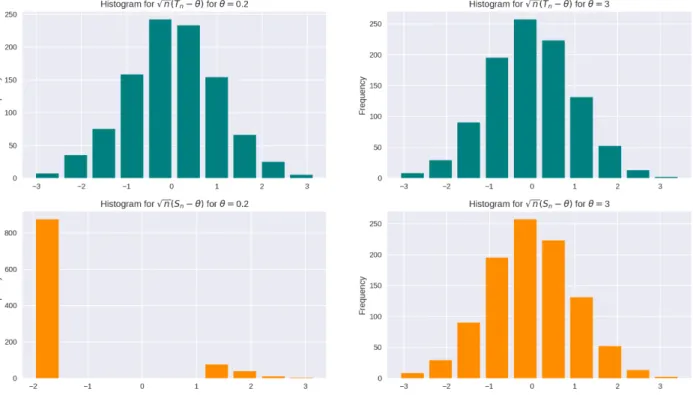
example is that shrinkage might affect not only asymptotic behaviour, but can also change finite-sample properties in a drastic manner, as the histograms show in the next figure.3
Figure 1: Lack of uniformity in the convergence to the limit distribution of Hodges Estimator
We see that the green histograms are very similar. This happens because Tn is not cursed by
non-uniform approximations. Differently, the orange ones show clearly different distributions. At θ = 0.2, the event {Sn = Tn} happens less often and we have different distributions. At θ = 3, a large enough
value for θ, the Hodges estimator generates a histogram that is similar to the one generated by Tn.
As useful as shrinkage estimators can be, we should take non-uniformities into consideration when approximating the finite-sample distribution by asymptotic distributions.
4.4 An Example of Model Selection and Non-Uniformity
As [Leeb and Pötscher, 2005] point out, although the Hodges estimator appeared in the statistical literature as a counter-example to the belief that MLE’s were in general the most efficient estimators, the type of anomaly it represents draws connections with the model selection environment. In order to see such connections, consider the following example, adapted from [Leeb and Pötscher, 2005].
Take the linear regression model
yt= αxt+ βzt+ et
where the usual conditions apply: et is iid N(0, σ2), (xt, zt) are scalar non-stochastic regressors and
the n × 2 matrix of regressors X is such that X′X/n → Q, with Q positive definite. For notational
convenience, let σ2(X′X/n)−1= ' σα2 σα,β σα,β σ2β (
in which the 3 parameters of this reduced-form matrix may depend on n but the subscript is omitted. The above setup is similar to the one we would encounter in a standard factor model in empirical asset pricing. Let’s say we are interested on the value α but we are not sure if β = 0 or not. If we think of xt= 1 and ztas a given factor, this is analogous the problem found in [Kozak et al., 2018b] (indeed in
a very simplistic exposition) where we are interested on assessing a factor model in terms of short-term α-returns but are including many risk factors that may well carry no pricing information. The main difference is that financial data is not iid.
We are faced with the decision to use the unrestricted model (call it U) with 2 unknown parameters (we assume that σ2 is known) or the restricted model (call it R) with β = 0 to fit data. In order to
choose between them, we use the following model selection scheme: we estimate the unrestricted model and check if |√n ˆβ(U )/σβ| > cn, where cn is a user-specified threshold, allowed to change with n. Let
M0 represent the true model:
M0 = $ % & R, if β = 0 U, if β ∕= 0 The result the model selection mechanism is cast by ˆM:
ˆ
M = U ⇐⇒ |√n ˆβ(U )/σβ| > cn
The post-model-selection estimator for α is ˜
α = ˆα(R)1M =Rˆ + ˆα(U )1M =Uˆ
An important detail is the choice of the sequence cn. A reasonable goal to a model selection mechanism
is the consistent estimation of the parameter d, following the notation from Section4.1. In this case, making the correct call between the restricted and the unrestricted model. This in controlled by the sequence cn.
4.4.1 Choosing the Sequence cn: A general result
Let’s suppose the data is generated by a distribution Pθ, with θ ∈ Rq. Here, the parameter d is
associated with the number of entries in θ that are truly 0: let I0 ={d+1, · · · , q} and I1 ={1, 2, · · · , d}
be the sets of indices that correspond to null entries and to non-zero entries, respectively.4 To each θ i
we associate an estimator ˆθi,n.
4We can always reorder the parameters to achieve such a setting. The fact that there is a cut-off between zero and
Also, consider sequences of positive numbers {σi,n, i = 1,· · · , q < +∞} that are consistently estimated
by ˆσi,n. Most likely, the sequence of interest for σi,n relates to the standard deviation of the
corre-sponding estimator, but there’s no gain on restricting the analysis to this case. We estimate I0 by
ˆ
I0 ={1 ≤ i ≤ q : |ˆθi,n|/ˆσi,n< ci,n}, in which ci,n is a deterministic sequence of real numbers that we
define for each i. The following result is adapted from [Bauer et al., 1988]: Theorem 1. Assume that
1. E(ˆθi,n− θi)2/σi,n2 is bounded for every i = 1, · · · , q.
2. ˆσi,n
σi,n
p
−
→ 1, for each i = 1, · · · , q.
3. ci,n→ +∞ and σi,nci,n→ 0, for every i = 1, · · · , q.
Then P( ˆI0 ∕= I0)→ 0. In other words, we can consistently estimate d.
Proof. Let i ∈ I0 and δ > 0. By Markov’s Inequality and 1), it follows that
P(|ˆθi,n|/(σi,nci,n) > δ)≤ δ−2E(ˆθ2i,n)c−2i,nσi,n−2≤ δ−2c−2i,nM
for some positive M. By 3), this implies that |ˆθi,n|/(σi,nci,n) converges in probability to zero. Then,
the same is true for |ˆθi,n|/(ˆσi,nci,n). This implies that for δ = 1 we have that
P(|ˆθi,n|/(ˆσi,n) > ci,n) =P(i ∕∈ ˆI0)→ 0
On the other hand, let i ∈ I1 and δ ∈ (0, 1). Then,
P(|ˆθi,n|/ˆσi,n≤ ci,n)≤ P(|ˆθi,n|σ−1i,nσi,nσˆi,n−1 ≤ ci,n,|ˆσi,n/σi,n− 1| < δ) + P(|ˆσi,n/σi,n− 1| ≥ δ)
The last term is approaching zero by 2). The first too:
P(|ˆθi,n|σ−1i,nσi,nσˆi,n−1≤ ci,n,|ˆσi,n/σi,n− 1| < δ) ≤ P(|ˆθi,n|σ−1i,n(1 + δ)−1 ≤ ci,n)
≤ P(|ˆθi,n− θi|/σi,n>−ci,n(1 + δ) +|θi|/σi,n)
≤ E(ˆθi,n− θi)2(−ci,nσi,n(1 + δ) +|θi|)−2
in which the second inequality follows by the triangular inequality. The last term eventually vanishes because 1), 2) and 3) imply convergence of ˆθi,n in quadratic mean and θi ∕= 0 by hypothesis. Hence
P(i ∈ ˆI0)→ 0
For each i, ci,n must increase with n but not too fast. The intuition is the following: if ci,n = α
(constant), as one could suggested in the spirit of a Wald test, the model selection procedure would choose the wrong model with positive probability even if n → +∞. After all, the asymptotic size of the test cast by ˆM would be fixed. If ci,n → +∞, the asymptotic size is zero. However, ci,n
cannot increase too fast otherwise the probability of a Type 2 will increase, which would also break the consistent estimation goal. Notice that the result does not tell us anything about “optimal” sequences.
4.4.2 Non-uniformity Arises
Back to the linear regression example, if cn→ ∞ and cn/√n→ 0, we are under the hypothesis of the
previous theorem and it holds that lim
n→∞Pn,α,β( ˆM = M0) = 1
where the limit above is taken point-wise in (α, β). Because { ˆM = M0} ⊂ {˜α = ˆα(M0)}, it follows that lim
n→∞Pn,α,β( ˜α = ˆα(M0)) = 1. The main
implica-tion is that the asymptotic distribuimplica-tion of ˜α will be the same as ˆα(M0). This property is often called
the “Oracle Property”, alluding to the fact that the true model can be uncovered with probability approaching one. But this convergence happens point-wise in the true parameter vector (α, β). According to this result, we could hope, exactly because we can consistently uncover the true model, that inference about the parameters can be done in the usual way. However, ˜α is nothing more than a variation of Hodges’ Estimator. The “shrinkage” here occurs towards the estimate of the restricted model. We should expected the same sort of strange finite-sample behaviour due to the lack of uniformity in the convergence results above with respect to the true parameters (α, β). The results won’t hold if we consider, as before, perturbations around β = 0 of a certain order.
If β ∕= 0, Pn,α,β( ˆM = M0) = 1−[Φ(cn−√nβ/σβ)−Φ(−cn−√nβ/σβ)]→ 1. But how fast we approach
1 depends crucially on how distant β is from zero. As before, consider a sequence of true parameters βn= hσβcn/√n, with |h| < 1. Now:
Pn,α,β( ˆM = M0) = 1− [Φ(cn(1− h)) − Φ(−cn(1 + h))]→ 0
because cn → +∞. The model selection mechanism is somewhat blind to some deviations of the
restricted model! Such behavior resembles the one seen in the Hodges estimator case.
A possible argument against the relevance of such example is that we need β close to zero (in fact converging to zero at a certain rate) in order to observe such an anomaly. Hence, as n grows, we would have, in theory, only slight misspecification. Yet, this finite-sample anomaly appears on the distribution of√n( ˜α− α), since the model selection scheme is fooled by perturbations of the order of 1/√n. This dependence on β propagates to finite-sample distortions over the distribution of√n( ˜α−α). The finite-sample density of√n( ˜α−α) is derived in [Leeb and Pötscher, 2005], where ρ = σα,β/σασβ ∕=
0 by assumption, ∆(a, b) = Φ(a + b) − Φ(a − b) and φ represents the pdf of the standard normal distribution: gn,α,β(u) = σ−1α (1− ρ2)−1/2φ(u(1− ρ2)−1/2/σα+ ρ(1− ρ2)−1/2√nβ/σβ)× ∆(√nβ/σβ, cn)+ σ−1α ) 1− ∆ )√ nβ/σβ + ρu/σα * 1− ρ2 , cn * 1− ρ2 ++ φ(u/σα).
The dependence on the unknown parameter β implies that the approximation √n( ˜α− α) towards its limit distribution (which is Gaussian, no matter the value of β) will also suffer from non-uniformity.
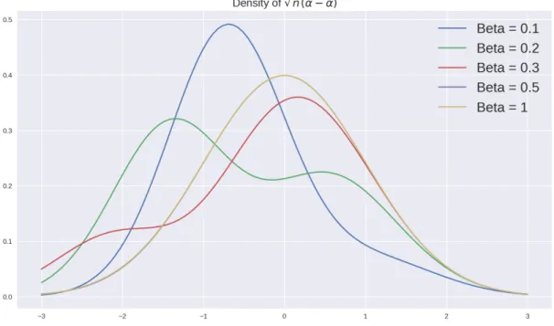
Figure 2: Finite-sample density of √n( ˜α− α)
For β = 1, the corresponding pdf resembles a Gaussian pdf, indicating that the approximation is good. However, there are cases in which we can even spot bi-modal densities, hinting at the problem of point-wise asymptotic theory.
As we could expect, the “naive” confidence intervals will display anomalies regarding coverage proba-bility since they rely on a point-wise asymptotic approximations. Let 1 − η be the nominal coverage probability (say, 95%). The corresponding confidence intervals for α based on ˜α are:
IR={˜α− zη/√n× σα(1− ρ2)1/2, ˜α + zη/√n× σα(1− ρ2)1/2}
IU ={˜α− zη/√n× σα, ˜α + zη/√n× σα}
where zηstands for the(1−η/2)-quantile of a standard normal distribution. For fixed (α, β) the coverage
probability Pn,α,β(α∈ I) converges to 1 − η. But again, this approximation happens point-wise.
The coverage probability satisfies:
Pn,α,β(α∈ I) = Pn,α,β(α∈ IR| ˆM = R)Pn,α,β( ˆM = R) +Pn,α,β(α∈ IU| ˆM = U )Pn,α,β( ˆM = U )
[Leeb and Pötscher, 2005] provide the exact coverage probability: Pn,α,β(α∈ I) = ∆(ρ(1 − ρ2)−1/2√nβ/σβ, zη)∆(√nβ/σβ, cn) + zη # −zη (1− ∆((√nβ/σβ+ ρu)(1− ρ2)−1/2), cn(1− ρ2)−1/2)φ(u)du
In order to prove the next theorem, we prove the following lemma:
Proof. In this case,
Pn,α,βn( ˆM = R) = Φ(cn(1− γn/cn))− Φ(−cn(1 + γn/cn))
So Pn,α,βn( ˆM = R)→ 1 since cn→ +∞. The result follows.
Define the infimal coverage probability µ as µ = lim
n→+∞infα,βPn,α,β(α∈ I)
Now we can prove an interesting result.
Theorem 2. Further allow γn→ +∞. Under this setting, µ = 0.
Proof. Let α be arbitrary and βn= σβγn/√n. By the previous lemma
lim n→∞infα,βPn,α,β(α∈ I) ≤ limn→∞Pn,α,βn(α∈ IR| ˆM = R)Pn,α,βn( ˆM = R) = lim n→∞∆(ρ(1− ρ 2)−1/2γ n, zη)∆(γn, cn) = 0 as γn→ +∞ and γn= o(cn).
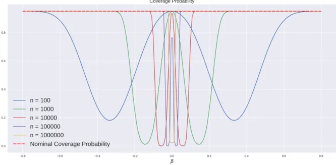
The cost of using a post-model-selection estimator is the lack of regularity not only in terms of conver-gence to the limit law but also to the nominal coverage probability of associated confidence intervals. Since this model selection scheme is fooled by perturbations around β = 0 of the order 1/√n, the standard confidence intervals will also have trouble dealing with such perturbations. The Figure 3
shows the coverage probability for different sample sizes and different values of β and 1 − η = 95%. Notice that it does not depend on α, but the exact value is heavily dependent on β, a parameter we are also estimating.
The plot suggests that no matter how big the sample size is, there will a value for β that will generate low coverage probabilities in a finite sample. The behaviour is symmetric around zero since the model selection scheme is only concerned with | ˆβ(U)|.
Moreover, the beheavior is not monotonic in β. For values very close to zero or really further away, the coverage probability is closer to its nominal value. However, if β is only “moderate” in the sense that’s it’s neither further away nor too close to zero, the coverage probability can be really low. Intuitively this is the case in which the model selection scheme is stressed at the most: it is in a scenario where data is not clearly generated by restricted or the unrestricted model. Despite of the simple design in which this example takes place, we provide some generalizations below. There’s nothing to make us hopeful that such non-uniformity problems will disappear in more complicated designs.
4.5 Confidence Sets, Maximal Risk and Sparse Estimators
When dealing with multi-dimensional data, as is the case of interest in the context of empirical asset pricing, the usage of LASSO-type estimators imply further problems for statistical inference that are
Figure 3: Lack of uniformity in the convergence to the nominal coverage probability (95%) of the “naive” confidence interval.
closely related to the “Oracle Property” and the lack of uniformity in the asymptotic approximations. After all, LASSO-type estimators perform model selection by design. The nature of these estimators is not different from the nature of the Hodges estimator, as noticed by [Bickel et al., 2009]. We establish a couple more results showing that non-uniform approximations towards limit laws is not a small problem regarding inference.
If even in the simple setup of the preceding example we could observe finite-sample anomalies, there’s little hope that these difficulties will disappear in more general scenarios. In fact, [Pötscher, 2008] shows that the problem of non-uniformity for sparse estimators has important consequences regarding the size of confidence sets.
The technique of using moving parameters, interpreted as perturbations around a point of interest such as 0, makes it possible to capture finite-sample anomalies, as in the example above and also as in the case of the Hodges Estimator. Consider a sequence of probability measures
,
Pn,θ : θ∈ Rk
-, n = 1, 2,· · ·
where these probabilities are defined on suitable measure spaces (Ωn,Fn). In a regression problem, for
instance, we can think about θ as the true coefficients and about n as the sample size.
Definition 1 (Contiguity). Given a sequence of measure spaces (Ωn,Fn) and two sequences of
prob-ability measures {Pn} and {Qn} defined on these spaces for each n, we say that the sequence {Qn}
is contiguous with respect to {Pn} if, for any sequence of measurable sets An ∈ Fn, the following
implication holds:
We assume that the sequence of probability measures ,
Pn,γ/√n: n = 1, 2,· · ·
-(7)
is contiguous with respect to
{Pn,0: n = 1, 2,· · · } (8)
for every fixed γ ∈ Rk. This is a weak assumption that will be satisfied, for example, when dealing
with Gaussian distributions as a direct application of Le Cam’s First Lemma. Further references on contiguity are [Cam and Yang, 2000] and [Duchi, 2018].
Now, let ˆθn∈ Rk denote a sequence of estimators for θ.
Definition 2 (Sparsity). The sequence of estimators ˆθn is sparse if for every θ ∈ Rk and i = 1, 2, ..., k
lim n→∞Pn,θ . ˆ θi,n= 0 / = 1, if θi= 0
where θi is the i-th component of θ.
LASSO-type estimators and estimators based on hard thresholds, as the one in the example before, display this property. This is different from standard consistency, and neither is implied by it nor is a sufficient condition for consistency. In a gaussian linear regression problem, for instance, the above limit is always zero, but the OLS estimator is consistent. On the other hand, ˆθn≡ 0 is certainly sparse
although not consistent for θ.
We are interested in confidence sets Cn= Cn(ω)⊂ Rk for θ that use the information provided by ˆθn.
In the definition below, n is taken as fixed.
Definition 3. The random set Cn is based on ˆθn if
Pn,θ . ˆ θn∈ Cn / = 1 for every θ ∈ Rk.
Finally, given a set A ⊂ Rk we can define its diameter and extension in a given direction. Considering
the euclidean norm, let
diam(A) = sup{||x − y|| : x, y ∈ A} and, given a ∈ A and a unit-vector e ∈ Rk, let
ext(A, a, e) = sup
λ {λ ≥ 0 : a + λe ∈ A}
The next result establishes that confidence sets based on sparse estimators are necessarily large and is due to [Pötscher, 2008]:
Theorem 3. Assume (7) is contiguous with respect to (8) for any γ ∈ Rk. Let {C
n}n∈Nbe a sequence of
random sets based on the sequence of sparse estimators ˆθn with asymptotic infimal coverage probability
δ > 0:
lim inf
n→∞ θinf∈RkPn,θ(θ∈ Cn) = δ
Then, for every t ≥ 0 and every unit-vector e ∈ Rk
lim inf n→∞ θ∈RsupkPn,θ .√ n· ext(Cn, ˆθn, e)≥ t / ≥ δ Also, this implies
lim inf n→∞ θsup∈RkPn,θ !√ n· diam(Cn)≥ t " ≥ δ
Proof. It’s trivially true that diam(Cn)≥ ext(Cn, ˆθn, e)holds with Pn,θ-probability 1 for all θ. Hence,
it’s enough to prove the first assertion. For any sequence θn, it follows that
δ ≤ lim inf n→∞ Pn,θn(θn∈ Cn) = lim inf n→∞ , Pn,θn . θn∈ Cn, ˆθn= 0, ˆθn∈ Cn / +Pn,θn . θn∈ Cn, ˆθn∕= 0
/-Choose γ ∈ Rk and let θ
n= γ/√n. Sparsity and contiguity, together, imply that
Pn,θn
.
θn∈ Cn, ˆθn∕= 0
/ → 0 Moreover, the following inclusion is valid
{θn∈ Cn, ˆθn= 0, ˆθn∈ Cn} ⊆ {ext(Cn, ˆθn, θn/||θn||) ≥ ||θn||} But ||θn|| = ||γ||/√n. Then, Pn,θn . θn∈ Cn, ˆθn= 0, ˆθn∈ Cn / ≤ P(√n· ext(Cn, ˆθn, γ/||γ||) ≥ ||γ||)
Given t ≥ 0 and e ∈ Rk of length 1, we can always choose γ = t · e and have the result.
Intuitively, this theorem implies that the confidence sets Cnmust be large in order to accommodate an
asymptotic infimal coverage probability of δ > 0. To understand how challenging the result is, suppose k = 1 and consider a confidence interval of the form Cn = [ˆθn− an, ˆθn+ an]. Then, diam(Cn) = 2an
and, for any t ≥ 0:
lim inf n→∞ θ∈RsupkPn,θ !√ n· an≥ t " ≥ δ
If an is not random, it must hold that lim inf√n· an = +∞. Hence, the boundary must shrink at
a rate less than √n. In comparison, in a normal regression problem, if we use a t-test to construct a confidence interval, √n times the diameter will be stochastically bounded, uniformly in θ, a way different scenario than this one. A corollary of this result is that any confidence interval such that √
n·diam(Cn)is uniformly stochastically bounded in θ necessarily has zero asymptotic infimal coverage
Therefore, when making inference in Machine Learning models that deploy L1-regularization techniques
such as the LASSO, the confidence intervals associated to the standard t-statistics (the “naive” ones) will have zero asymptotic infimal coverage probability. The point-wise convergence to the nominal coverage probability is not uniform at all. The next result strengths this observation. The rate √nis not the correct one for such estimators in order to obtain the asymptotic distributions:
Theorem 4. Suppose that the contiguity hypothesis is valid and that the sequence of estimators ˆθn is
sparse. Then, for any M ∈ R we have lim inf n→∞ θsup∈RkPn,θ .√ n· ||ˆθn− θ|| ≥ M / = 1
Proof. Notice that for a sequence θn= γ/√n with ||γ|| > M, it holds that
lim inf n→∞ θsup∈RkPn,θ .√ n· ||ˆθn− θ|| ≥ M / ≥ lim infn →∞ Pn,θn .√ n· ||ˆθn− θn|| ≥ M / ≥ lim inf n→∞ Pn,θn .√ n· ||ˆθn− θn|| ≥ M, ˆθn= 0 / = lim inf n→∞ Pn,θn . ˆ θn= 0 /
From the sparsity assumption
Pn,0 . ˆ θn= 0 / → 1 Then, the result follows by the contiguity assumption.
The previous example of the Hodges’ Estimator showed that it dominated the sample mean in terms of asymptotic risk, for a wide range of loss functions. However, as one should anticipate in light of all problems above regarding sparse estimators, asymptotic approximations can be misleading for a risk analysis. If one considers moving parameters as in the previous theorems, anomalies in terms of finite-sample risk (in special, finite-sample MSE) can be found. Actually, as [Leeb and Pötscher, 2008] highlight, whatever the loss function used, the maximal (scaled) risk of a sparse estimator is as bad as it possibly can be - even in large samples. The next theorem, adapted from [Leeb and Pötscher, 2008], makes this claim precise.
Theorem 5. Let ˆθn be a sparse sequence of estimators for θ ∈ Rk. Assume that (7) is contiguous with
respect to (8) for any γ ∈ Rk. Then, for any non-negative loss-function l : Rk→ R, it holds that
sup θ∈RkEn,θ . l.√n.θˆn− θ /// → sup s∈Rk l(s) as n → +∞. If l is unbounded, the (scaled) risk diverges to +∞.
Proof. The technique is the same as before, which consists of using a wise sequence of parameters that uncovers the anomalies. Let γ ∈ Rk and choose θ
n=−γ/√n. Then: sup s∈Rk l(s)≥ sup θ∈RkEn,θ . l.√n.θˆn− θ /// ≥ En,θn . l.√n.θˆn− θn /// ≥ En,θn . l.√n.θˆn− θn // 1θˆn=0 / = l(γ)Pn,θn . ˆ θn= 0 /
But Pn,0
. ˆ θn= 0
/
→ 1 by the sparsity property. From contiguity, Pn,θn
. ˆ θn= 0
/
→ 1. Since γ was arbitrary, the proof is done.
If l is usual quadratic function, the result above implies that the (scaled) MSE of sparse estimators for models in which the contiguity assumption is satisfied is unbounded. Scaling is necessary, otherwise convergence in quadratic mean would make it impossible to observe such an anomaly. For the normal linear regression problem, the√n-scaled MSE remains bounded as the sample size increases:
En,θn 0 n.θˆOLS − θn /′. ˆ θOLS − θn /1 =trace2!X′X/n"−13
which converges to trace(Q) < +∞ as long as (X′X/n)−1 → Q. The next simulation portrays this
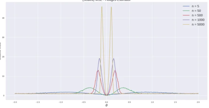
problem for the Hodges’ Estimator. No matter how big the sample size is, the spikes in the MSE will be present and will be each time higher as n approaches +∞, exactly the result pinned down by the last theorem.
Figure 4: Maximal MSE is bad as it can be for sparse estimators, in special for the Hodges’ Estimator The last results and simulations show that shrinkage estimators, due to their sparsity, create problems for point-wise asymptotic theory. The next section turns back to the original problem of estimating risk prices using LASSO estimators, taking care of these anomalies.
5 Uniformly Valid Inference For Linear Factor Models
The usual practice in empirical asset pricing is to consider factor models for the stochastic discount factor or directly for the asset returns. Where to begin with is only a choice of language since we can always derive the implicit linear model for the SDF once we have chosen a linear model for returns
and vice-versa. [Cochrane, 2005] highlights however that there is a fundamental difference between the risk price and the risk premium commanded by a given factor. The former is concerned with the amount of extra return an asset is expected to obtain once marginally more exposed to a given factor. The latter is related to the price of hedging against a given factor solely because it might be related to asset returns without explicitly driving them. It’s another incarnation of the causality-correlation duality.
As [Cochrane, 2005] points out, the correct measures to assess the influence of a newly proposed factor over a set of asset returns are risk prices, since a factor is useful or not as long as it’s capa-ble of driving returns (or the SDF). However, as discussed in [Cochrane, 2011] and more recently in [Harvey et al., 2016], the empirical asset pricing literature has come up with possibly too many factors to explain asset returns, raising three main questions. First, under a huge number of possible choices, how should the practitioner choose which factors to include when building a factor model? Next, how to estimate such a model without overfitting data becomes a central theme, specially if the hypothesis of truly high-dimensional models is entertained. Last, how to assess the pricing information eventually carried by a newly proposed factor once the contribution of previously chosen factors has been already accounted for?
Model selection techniques from the Machine Learning literature can certainly help answering the first two questions, such as the LASSO [Tibshirani, 1996] and the Elastic Net [Zou and Hastie, 2005]. How-ever, there is no free lunch in terms of statistical inference. Although the geometry of such estimators implicitly operates model selection and we have efficient algorithms to estimate them - targeting the first two problems - inference on estimated parameters is cursed by non-uniform asymptotics. This happens because these are sparse estimators, in general. As seen in the previous section, this brings along anomalies regarding non-uniformity.
Such anomalies related to non-uniform asymptotics are not new in Economics. The fact that there exist estimators whose convergence to limit distributions do not happen uniformly over the parameter space is well-known. For instance, this kind of challenge appears in theory of Instrumental Variable Estima-tors when instruments are weak and also in auto-regressive models with nearly-integrated regressors. Main references for these cases are [Andrews et al., 2006] and [Jansson and Moreira, 2006].
When using sparse estimators for model selection, the central problem regarding statistical inference is that such model selection schemes choose the incorrect model with positive probability for any finite sample. In a linear regression framework, where model selection means selecting the appropriate controls in a data-driven way, this can generate omitted-variable bias. It’s expected that these mistakes become less likely as the sample size increases. Nonetheless, the convergence in the LASSO case is not fast enough for standard asymptotic theory kick in, for example.
Along the task of choosing a model specification and estimating it, with a linear factor model as an application, some sort of Occam’s Razor principle comes into play. Simpler models are less prone to overfit data and can be estimated more precisely, which generally leads to better out-of-sample performance. But we can’t afford accepting too few factors as relevant controls since omitted-variable
bias might become a problem, making correct inference about risk prices an impossible task. More than that, it’s possible that a newly proposed factor is almost perfectly spanned by other factors already considered by the practitioner and its inclusion could generate only slight improvements on pricing at the cost of overall statistical precision. Hence, model selection, estimation and inference should be embedded in the same framework since these are connected problems. We seek simple models but ones that are just simple enough and produce reliable statistics for inference.
These Machine Learning techniques were created for prediction tasks, and it’s not surprising that some modifications must be made in order to use them to draw inference about estimated parameters. Thankfully, research on the econometric theory of high-dimensional models is a thriving field with many recent developments, as reviewed in [Belloni et al., 2015]. Recently, [Feng et al., 2019] adapted the results from [Belloni and Chernozhukov, 2013] and [Belloni and Chernozhukov, 2014] to a factor model setup that can help answering the third and most important question from above.
For convenience, we restate the model from Section3. The main equation to be estimated is equation (2):
E(rt) = 1nγ0+ Cgλg+ Chλh
in which rt represent a n × 1 vector of returns, γ0 is a zero-beta rate, λg and λh are risk prices and Cg
and Ch are covariances between returns and factors. We also write the following projections:
gt= ηht+ zt, where Cov(ht, zt) = 0
Cg = 1nξ⊺+ Chχ⊺+ Ce
where η is a d × p projection matrix, ξ is a d × 1 vector, χ is a d × p projection matrix and Ce is a
n× d matrix of cross-sectional residuals.
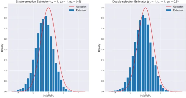
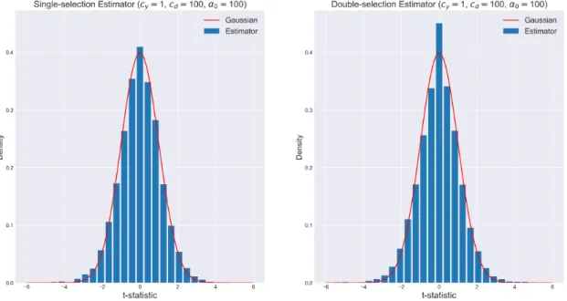
5.1 Single vs Double-Selection Estimator
The original LASSO estimator from [Tibshirani, 1996] entails a L1-penalty on estimated parameters.
It’s a way of trading-off bias for variance, leading to an estimator that outputs many zeros as coefficients for the righ-hand-side variables seen as least important to explain the variation of the dependent variable. This seems promising if one is interested to perform model selection and is willing to deal with biased coefficients, an acceptable trade-off on some prediction-only tasks. Nonetheless, if inference on estimated parameters is to be performed, then matters are more complex since correcting this bias is not trivial.
[Belloni and Chernozhukov, 2013] provide theoretical and simulation results arguing against the stan-dard LASSO and proposing the Post-LASSO for this type of linear setup. They proposed to separate the model selection phase from the estimation phase. This enhanced version first runs a standard LASSO regression over the full set of parameters and then runs a second step OLS regression of the dependent variable over the independent variables whose coefficients were non-zero in the first stage. If the first stage selects the correct model, then the OLS estimates of the second stage are unbiased