An Automatic Methodology for Obtaining Optimum Shape Factors for the Radial Point Interpolation Method

An Automatic Methodology for Obtaining Optimum

Shape Factors for the Radial Point Interpolation

Method

Péricles L. Machado, Rodrigo M.S. de Oliveira, Washington C.B. Souza, Ramon C.F. Araújo, Maria E.L. Tostes Universidade Federal do Pará (UFPA)−Instituto de Tecnologia (ITEC)−Belém, Pará, Brazil

pericles.raskolnikoff@gmail.com, rmso@ufpa.br, csaksousa@yahoo.com.br, ramon.araujo@itec.ufpa.br and tostes@ufpa.br

Cláudio Gonçalves

Universidade do Estado do Amazonas−Manaus, Amazonas, Brazil

gonca.claudio@gmail.com

Abstract − In this letter, a methodology is proposed for automatically (and locally) obtaining the shape factor c for the Gaussian basis functions, for each support domain, in order to increase numerical precision and mainly to avoid matrix inversion impossibilities. The concept of calibration function is introduced,

which is used for obtaining c. The methodology developed was applied for a 2-D

numerical experiment, which results are compared to analytical solution. This comparison revels that the results associated to the developed methodology are very close to the analytical solution for the entire bandwidth of the excitation pulse. The proposed methodology is called in this work Local Shape Factor

Calibration Method (LSFCM).

Index Terms −improved numerical precision, matrix inversion difficulties, optimum shape factor calculation, radial point interpolation method (RPIM).

I. INTRODUCTION

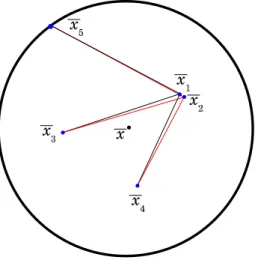
Figure 1. Support domainΩwith eight nodes (k=8).

As it is well known, Gaussian, multiquadrics, logarithmic and splines functions are used in RPIM method as basis functions that depend on an arbitrary parameters [9]. In particular, Gaussian basis depends on a free parameter c, known as the shape factor, which affects the accuracy of the interpolation of functions of interest in a particular support domain. In previous works [3], [8], the parameter c is defined globally usually as c=0.01. However, this value is not adequate for every support domain, due to loss of accuracy and especially due to matrix inversion impossibilities [9]. This issue has been treated in literature by using methods such as the leave-one-out-cross-validation algorithm (LOOCV) [9], [10], [11], which calculates a optimum global shape parameter by using statistical analysis.

In order to improve the accuracy of the RPIM method, this paper presents a formulation for computing c in an automatic way, locally for each support domain (Fig. 1), in such way reduced interpolation errors are obtained and matrix inversion difficulties are avoided. This is accomplished by using a high frequency signal, called here calibration function. This way, the proposed method is namedLocal Shape Factor Calibration Method (LSFCM). Excellent agreements to analytical solution were observed.

II. REVIEW OF THE RPIM METHOD

Consider a function u(x) in space. This function can be interpolated in a support domainΩcentered at x by

u(x) = k

∑

i=1

ri(x)ai+ M

∑

j=1

pj(x)bj=RT(x)a+PT(x)b, (1)

in whichri(x) =e−c(r/rmax)2 is the Gaussian radial basis function,r=p(x−xi)2_{+ (y−yi)}2_{,c>0 is the shape factor} and rmax is the maximum value assumed by r in Ω. Here, xi is the ith node of Ω, i=1,2, ...,k and PT(x) is a

polynomial function with M terms. In this work, PT_{(x) is given by [1,x,y]and M=3.}

When (1) is considered for all nodes inΩ, one obtains the matrix equation

where,Ro= [RT(x1),RT(x2), ...,RT(xk)]T andPo= [PT(x1),PT(x2), ...,PT(xk)]T, withxi∈Ω,i=1...kandUs contains

all the values assumed by u(xi) in Ω.

In order to ensure that a unique solution is obtained for a and b in (2), the condition P_oTa=0 is imposed [3]. With some algebra, it can be shown that

b= [PoTR− 1 o Po]−

1

PoTR− 1

o Us=SbUs (3)

and

a= (R−1_o −R−1_o PoSb)Us=SaUs. (4)

This way, (1) can also be written as

u(x) = [RT(x)Sa+PT(x)Sb]Us=Ψ(x)Us, (5)

in which Ψ(x) is a vector containing samples of shape functions associated to each nodeiin Ω. It is important to mention that the shape functions in Ωmust satisfy the Kronecker delta property [3], [9].

As far as Sa and Sb are constant matrices (because the nodes’ coordinates are fixed), the partial derivative of

Ψl(x) with respect to v is given by

∂Ψl

∂v =

k

∑

i=1

∂Ri

∂vS

a i,l+

M

∑

j=1

∂Pj

∂v S

b

j,l, (6)

where l=1...k, ∂Ψ_∂v = [∂Ψ1

∂v ,

∂Ψ2

∂v , ...,

∂Ψk

∂v ], S a

i,l is the element of matrix Sa indexed by (i,l), S b

j,l is the element of Sb

indexed by (j,l) andv=x orv=y. Finally, the partial derivative ofu with respect to v can be expressed by

∂u ∂v =

∂Ψ ∂vUs=

k

∑

i=1

∂Ψi

∂v us,i. (7)

In this work, Maxwell’s equations are solved in 2-D space, by considering the TMz mode [1]. The associated spatial derivatives are approximated by (7) and the field updating equations

Hn+

1 2

x,i =H n−1

2

x,i −

∆t µ

∑

n z,j∂yΨj

!

, (8)

Hn+

1 2

y,i =H n−1

2

y,i +

∆t µ

∑

n z,j∂xΨj

!

, (9)

E_zn_,+_i1=E_zn_,i+∆t

ε

∑

n+1 2

y,j ∂xΨj−

∑

Hn+

1 2

x,j ∂yΨj !

are obtained. In (8)-(10), central finite-differences are used to approximate the time derivatives.

Here, the UPML (Uniaxial-Perfectly Matched Layer) formulation developed by Gedney [12] was implemented for truncating the analysis domain.

III. THELOCALSHAPEFACTORCALIBRATIONMETHOD(LSFCM)

Previous works considerc≈0 as a global parameter [3], [8] (c=0.01 is often used). Although small values ofc can produce highly accurate results, it is not always possible to compute (8)-(10) due to matrix inversion difficulties [9]. This occurs because when a node is placed close enough to another in Ω, as illustrated by Fig. 2, and c is close to zero, the Gaussian basis functions tend to be constant (tend to the unity) between the mentioned nodes and thus the associated matrices tend to be non-invertible. Mathematically, because Ro in expanded form is given

by [9]

Ro= 

       

R1,1

o R1o,2 ... R1o,k

R2o,1 R2o,2 ... R2o,k

..

. ... . .. ... Rk,1

o Rko,2 ... Rko,k 

       

, (11)

in which Rio,j=exp −c(ri,j/rmax)2

and ri,j= p

(xi−xj)2+ (yi−yj)2, it is observable that for the case of Fig. 2,

the distances r1,n andr2,n (from nodes 1 and 2 to noden, respectively), with n>2, are approximately equal. This

way, it is evident thatR1o,n≈R2o,n. Additionally, whenc≈0,R2o,1≈Ro1,2≈exp(0) =1. Observing thatRo1,1=R2o,2=1,

it is easy to see that the situation depicted by Fig.2 makes the lines one and two of (11) almost linearly dependent, promoting inversion difficulties for Ro.

Figure 2. Example of support domain with two nodes positioned close to each other.

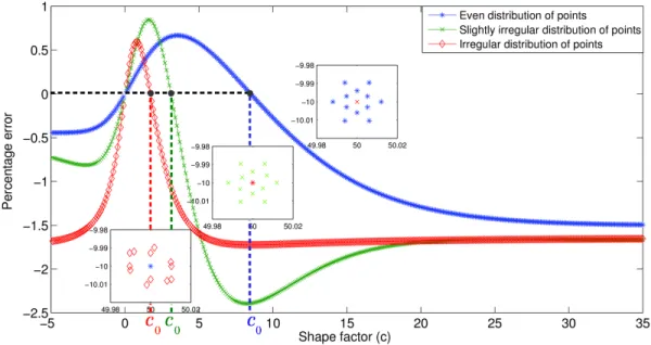
This procedure can be obtained if Fig.3 is carefully observed. It contains plots of the percentage interpolation error (E_{%) for a given signal u(x) as a function ofc for three different spatial arrangement of nodes: symmetrical}

(even), slightly irregular and irregular arrangements. As one can observe, as cgoes to zero, the interpolation tends to produce very low percentage errors for every case. However, the curve is discontinuous around c=0 due to the matrix inversion impossibilities in this range. Additionally, it is possible to observe that, for each case, a second root Co exists. The core idea of this work is to useCo as the shape factor for avoiding matrix inversion impossibilities

and, in addition, to improve the interpolation precision. In practice, as long as u(x) is not known analytically, the error function E _{cannot be calculateda priori.}

Based on the above discussion, an hypothesis has been formulated: given a function u(x) and its maximum significative frequency fmax, the frequency fmax can be used as a reference parameter for determiningCo forΩ, in

Figure 3. E_%versuscfor even, slightly irregular and irregular arrangements ofk=12 interpolating nodes foru(x¯) =C(x¯)and graphical definition ofCo.

This hypothesys can be verified if, for given a support domain Ω, a calibration functionC(xi,yi), given by

C(xi) =cos(Kxi) +sin(Kyi), (12)

is calculated for everyxi inΩ. In (12),xi= (xi,yi) represents theithnode in ΩandK is the associated wavenumber,

which is expressed by

K=2πfmax

v0

. (13)

In (13), v0 is the light speed in vacuum. In order to determineCo, the error

E_{(c) =Ci(c,x)−C(x) (14)}

is considered in this work. In (14),Ci(c,x), which is the interpolated version ofC(x), is obtained by using (1) and (12). From (14), the percentage error can be calculated by E_{%(c) =100(Ci(c,x)−C(x))/C(x). Therefore, we can}

say thatCo is a root of the percentage error, when the calibration function is considered, in such way thatCo>0.

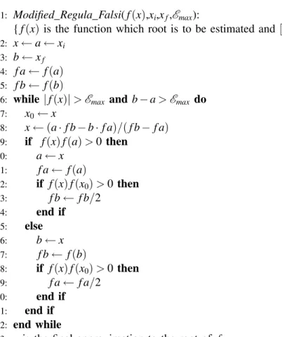
In this work, the modifiedregula falsi method [13] is used for determiningCo from (14), in such way that

C(x)−E_{max≤Ci(Co,x)≤C(x) +}E_{max. (15)}

by Fig.4.

1: Modified_Regula_Falsi(f(x),xi,xf,Emax):

{f(x) is the function which root is to be estimated and [xi,xf]is the root search interval}

2: x←a←xi

3: b←xf

4: f a← f(a)

5: f b← f(b)

6: while |f(x)|>E_{max and b−a>}E_{max do} 7: x0←x

8: x←(a·f b−b·f a)/(f b−f a)

9: if f(x)f(a)>0 then

10: a←x

11: f a← f(a)

12: if f(x)f(x0)>0 then

13: f b← f b/2

14: end if

15: else

16: b←x

17: f b← f(b)

18: if f(x)f(x0)>0 then

19: f a← f a/2

20: end if

21: end if

22: end while

23: x is the final approximation to the root of f.

Figure 4. The modifiedregula falsialgorithm.

In a few cases, it is not possible to determine if Co exists in the range 1≤c≤50 because E(50).E(1)>0

(in some cases it does not). For these cases, a minimization algorithm is performed for the function |E_{(c)|in the}

referred interval. IfCocan not be found in the initial searching range, a new interval is defined for the investigation

(e.g. 50≤c≤100). Finally, it is of fundamental importance to observe that the spatial derivatives in (8)-(10) are considered separately for determining the values assumed byCo.

IV. NUMERICALEXPERIMENTS ANDDISCUSSION

For the performed experiments, initially global values ofc were used for testing purposes (c=0.1, c=7.4 and c=8.5) with k=12. The average spacing among points is ∆a = ₁₇λ (Fig.5b), where λ=v0/fmax. Then, c was locally calculated (specifically for each support domain) by applying the methodology presented in this paper, and a new simulation was executed. For this case, the parameters ∆a andk were kept unchanged (∆a=₁₇λ andk=12).

The precision and stability criteria of the RPIM algorithm follows [8].

The problem was also solved analytically by using the solution presented by [14], and additional numerical data were generated by using the FDTD method. The Fourier transform was applyed to the transient signals in order to make the comparisons to the analytical solution feasible.

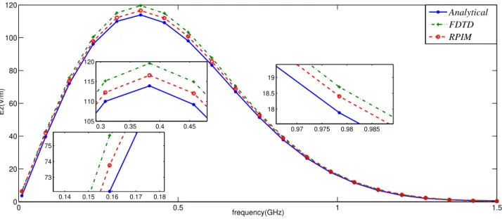
Fig.7 shows a graphical comparison among the analytical and numerical solutions for electric field at ℓx=20

mm, with ∆a=₁₇λ, for local and global shape parameters. For FDTD, due to the staircase effect, it was necessary

to discretize space with ∆=₈₀λ in order to get results closer to that generated with RPIM (∆a= ₁₇λ). Fig.8 shows

similar results for ℓx=38 mm.

In Figs.7 and 8, it is possible to see that the use of local valuesCo produces the closest curves to the analytical

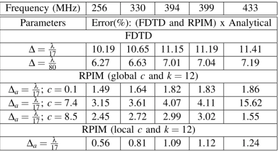
solution for the entire band of frequencies. When the RPIM method employs c=7.4, for example, it is possible to see errors E_{% of 15.62% for the higher frequency components. However, with the local shape factors Co, the}

RPIM algorithm produces a maximum error of 1.24% for ∆a=₁₇λ (see Tables I and II for numerical data regarding ℓx=20 mm).

Figure 5. (a) Geometric configuration of the problem and points used for calculatingEzand (b) part of the set of points used for representing the analysis region (~E and~Hare not calculated at the same points in space [8]).

0 2 4 6

−400 −200 0 200 400

time (ns) (a)

E (V/m)

0 0.5 1 1.5

0 50 100 150 200 250 300

frequency(GHz) (b)

E(V/m)

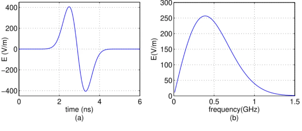
Figure 6. Wideband pulse used as the excitation source: (a) time domain, (b) its frequency spectrum.

Fig.5a defines the points where the electric field was calculated in this work, where ℓx is a distance measured

0 0.5 1 1.5 0 10 20 30 40 50 60 70 80 90 100 frequency(GHz) Ez(V/m) Analytical FDTD

RPIM with local c RPIM with c = 0.1 RPIM with c = 7.4 RPIM with c = 8.5

0.2 0.3 0.4 0.5

70 75 80 85 90

0.4 0.45 0.5 0.55 72 74 76 78 80 82

0.85 0.9 0.95 1

12 14 16 18 20 22 24

Figure 7. Analytical and numerical solutions for~E atℓx=20 mm: FDTD(∆=₁₇λ); RPIM(∆a=₁₇λ, localcand globalc(c=0.1,c=7.4

and c=8.5)).

0 0.5 1 1.5

0 20 40 60 80 100 120 frequency(GHz) Ez(V/m) Analytical FDTD RPIM

0.14 0.15 0.16 0.17 0.18 73

74 75

0.3 0.35 0.4 0.45 105

110 115 120

0.97 0.975 0.98 0.985 18

18.5 19

Table I

ANALYTICAL AND NUMERICAL RESULTS(ℓx=20MILIMETERS)

Frequency (MHz) 256 330 394 399 433

Parameters Ez (V/m)

Analytical Solution

[14] 73.87 81.47 82.30 82.16 80.53

FDTD

∆=₁₇λ 81.40 90.15 91.48 91.35 89.72

∆=₈₀λ 78.50 86.87 88.07 87.94 86.32

RPIM (globalc and k=12)

∆a=₁₇λ;c=0.1 74.97 82.81 83.80 83.66 82.03

∆a=₁₇λ;c=7.4 71.54 78.53 78.95 78.78 67.95

∆a=₁₇λ;c=8.5 72.06 79.25 79.84 79.68 79.28

RPIM (local c andk=12)

∆a=₁₇λ 74.28 82.13 83.20 83.08 81.53

Table II

PERCENTAGEERRORS OFNUMERICALMETHODS(ℓx=20MILIMETERS)

Frequency (MHz) 256 330 394 399 433

Parameters Error(%): (FDTD and RPIM) x Analytical FDTD

∆=₁₇λ 10.19 10.65 11.15 11.19 11.41

∆=₈₀λ 6.27 6.63 7.01 7.04 7.19 RPIM (globalc and k=12)

∆a= ₁₇λ;c=0.1 1.49 1.64 1.82 1.83 1.86

∆a= ₁₇λ;c=7.4 3.15 3.61 4.07 4.11 15.62

∆a= ₁₇λ;c=8.5 2.45 2.72 2.99 3.02 1.55

RPIM (local c andk=12)

Figure 9. Spatial distribution of log₁₀(Co)for calculating (a)∂Ez/∂xand (b)∂Ez/∂yfor the present problem.

Finally, Fig.9 shows the spatial distributions ofCo for the present problem. They were obtained for calculating

∂Ez/∂x (Fig.9a) and ∂Ez/∂y (Fig.9b) on (9) and (8), respectively. As previously discussed, it is possible to see in

Fig.9 that most values ofCo is in the initial searching range for c (from 1 to 50). However, in a few cases (mostly

near the cylinder’s border), where points are placed closer to each other, higher values of Co were obtained (red

points meansCo≈100, which is the maximum value assumed byCo in this example).

V. FINAL REMARKS

The results of the performed experiment confirm the hypothesis in this work: a calibration function can be used for calculatingCo, since it contains the higher frequency component of the signal to be propagated. The developed

methodology was computationally implemented and it was confirmed numerically that the procedure is suitable for automatically obtaining the shape factors of the Gaussian functions locally (for each support domain). Besides it makes the RPIM method more autonomic and more accurate for applications that involves multi-scale techniques, the new methodology prevents difficulties regarding matrices inversions associated to the use of small values of c. Although in this paper the developed methodology (LSFCM) has been developed numerically, it could be improved if analytical calculation ofCo can be performed. This would suppress the necessity of using root-finding

algorithms, such as the regula falsimethod used in this paper (the calculation ofCo increased the processing time

in approximately 25% for the numerical examples in this work).

VI. ACKNOWLEDGEMENTS

The authors are thankful to UFPA, to UEA and FAPEAM for infrastructure and financial support. We also acknowledge reviewers for all the valuable recommendations for improving the quality this paper.

REFERENCES

[1] A. Taflove and S. C. Hagness,Computational Electrodynamics, The Finite-Difference Time-Domain Method, 3rd ed. Artech House,

2005.

[2] K. Yee, “Numerical solution of initial boundary value problems involving Maxwell’s equations in isotropic media,” IEEE Trans.

Antennas and Propagation, vol. 14, pp. 302–307, 1966.

[3] J. G. Wang and G. R. Liu, “A point interpolation meshless method based on radial basis functions,”Int. J. Numer. Method, vol. 54,

pp. 1623–1648, 2002.

[4] Y. Yu and Z. Chen, “A 3-d radial point interpolation method for meshless time-domain modeling,”Microwave Theory and Techniques,

IEEE Transactions on, vol. 57, no. 8, pp. 2015 –2020, aug. 2009.

[5] X. Chen, Z. Chen, Y. Yu, and D. Su, “An unconditionally stable radial point interpolation meshless method with laguerre polynomials,”

Antennas and Propagation, IEEE Transactions on, vol. 59, no. 10, pp. 3756 –3763, oct. 2011.

[6] T. Kaufmann, C. Engstrom, C. Fumeaux, and R. Vahldieck, “Eigenvalue analysis and longtime stability of resonant structures for the

meshless radial point interpolation method in time domain,”Microwave Theory and Techniques, IEEE Transactions on, vol. 58, no. 12,

pp. 3399 –3408, dec. 2010.

[7] G. R. Liu and Y. T. Gu,An Introduction to Meshfree Methods and Their Programming. Springer, 2005.

[8] T. Kaufmann, C. Fumeaux, and R. Vahldieck, “The meshless radial point interpolation method for time-domain electromagnetics,” in

IEEE MTT-S International Microwave Symposium, 2008, pp. 61–65.

[9] G. E. Fasshauer,Meshfree Approximation Methods with MatLab. World Scientific Publishing Company, 2007.

[10] G. E. Fasshauer and J. G. Zhang, “On choosing "optimal" shape parameters for rbf approximation,” Numerical Algorithms, vol. 45,

no. 1-4, pp. 345–368, 2007.

[11] T. Kaufmann, C. Engstrom, and C. Fumeaux, “Residual-based adaptive refinement for meshless eigenvalue solvers,” inElectromagnetics

in Advanced Applications (ICEAA), 2010 International Conference on, 2010, pp. 244–247.

[12] S. D. Gedney, “An anisotropic perfectly matched layer absorbing media for the truncation of fdtd latices,”IEEE Trans. Antennas and

Propagation, vol. 44, pp. 1630–1639, 1996.

[13] S. C. Chapra and R. P. Canale,Numerical Methods for Engineers, 6th ed. McGraw-Hill, 2010.