F RANCISCO DEC ASTILHOM ONTEIROG

(1)

M

ESTRADO

M

ATEMÁTICA

F

INANCEIRA

TRABALHO FINAL DE MESTRADO

D

ISSERTAÇÃO

F

RACTIONAL

P

ROCESSES

:

A

N

A

PPLICATION TO

F

INANCE

F

RANCISCO DE

C

ASTILHO

M

ONTEIRO

G

IL

S

ERRANO

(2)

M

ESTRADO EM

M

ATEMÁTICA

F

INANCEIRA

TRABALHO FINAL DE MESTRADO

D

ISSERTAÇÃO

F

RACTIONAL

P

ROCESSES

:

A

N

A

PPLICATION TO

F

INANCE

F

RANCISCO DE

C

ASTILHO

M

ONTEIRO

G

IL

S

ERRANO

O

RIENTAÇÃO

:

J

OÃO

M

IGUEL

E

SPIGUINHA

G

UERRA

(3)

Abstract

In this work it is presented an extensive mathematical description oriented to financial modelling based

on three main fractional processes: the fractional Brownian motion and both fractional L´evy processes. It

is shown how these processes were originated. The concept of self-similarity is explored and we present

some notions of fractional calculus. It is discussed the opportunity of these processes in pricing financial

derivatives and we present a new approach for simulation of the fractional L´evy process, which allows a

Monte Carlo method for pricing financial derivatives.

Keywordsfractional processes; fractional Brownian motion; fractional L´evy process; simulation;

(4)

Acknowledgements

Agrade¸co à minha Mãe e ao meu Pai. Ao Salvador, ao Afonso e, claro, à Constan¸ca.

Agrade¸co ao Professor Jo˜ao Guerra a paciˆencia que teve com o seu orientando, assim como as suas

sugest˜oes e dedica¸c˜ao.

(5)

CONTENTS CONTENTS

1 Introduction

In the following few pages, we aim to introduce the subject of fractional stochastic processes that may be

considered a possible and original approach to the issue of pricing financial derivatives. This is actually

one of the final causes of this study. On a different (and greatly secondary, but not unimportant at

all) perspective, with this work we also hope to reach a phenomenologic or heuristic approach to some

understanding of the notion of mathematics itself: arguing that the mathematics has always a beginning

and an end necessarily in reality itself as a main claim, even for the most abstract mathematical subject,

or even if these endings are not known. One consequence is the refutation of the existence of a “world” of

mathematical objects as well as the notion of mathematics as just a (cruel) chess game. And this is still

possible when reaffirming the non-real proper existence of the mathematical objects: there is no ontological

difference between a real number and an imaginary number. Somehow, both objects are imaginary. But

they are the result of the same creativity that creates a portrait which is not the thing that represents,

just like it is mentioned by Magritte in his “La trahison des images”. But this creativity is always locked

up in reality in some sense. There is nothing new, in its absolute sense, as humanity will not ever create

anything. Mathematics is art.

Somehow, water was the first element to deliver a clue on one of the historically most important blocks

of financial mathematical modelling. This piece of knowledge is called the Brownian motion, named after

Robert Brown. In Brown (1828) the author describes the irregular movement of particles of pollen on

the surface of water. This description was later formally defined by Wiener, which was the cause of the

name of the stochastic process (Wiener process) whose trajectories are Brownian motions. Nevertheless,

it is commonly accepted to call Brownian motion to the process itself. The Wiener process is a stochastic

process with almost surely continuous paths in time, but these are almost surely not differentiable in each

instant. Also, the increments of this process are stationary, independent and Gaussian distributed.

The use of this process, whose historical origin is a natural phenomena in water, represented something

quite important and frequent in mathematics. We can call it the pursuit of simplicity. Since the prices

of financial assets (such as stocks) have mostly human causes, its variation and future value may be

influenced by a not easy composition of a quite large quantity of deterministic and non-deterministic free

human actions. Even if we admit a rational behaviour of economic agents in a perfect market (which is a

way to determine free human actions), we would still be left with a great problem to determine a theoretical

appropriate model, in a first place, followed by the huge problem to observe variables that (almost them)

cannot be observed.

At a first glance, with stochastic modelling, the deterministic complexity was substituted by simple

randomness.

Here we will present a mathematical phenomenon similar to the simplification earlier described. The

(8)

1 INTRODUCTION

observed in prices of stocks. But this irregularity is different from chaos. There are real physical causes

for the movements of the those particles and there are real human causes for the oscillations of the prices

in a market, even if we do not know them completely. This may be one of the reasons to abandon the

term irregularity (a close neighbour of chaos, which is the absence of causes) for another one, for instance,

roughness, a term proposed by Mandelbrot, which is a word often used to describe the surfaces of fractals.

On one hand, fractals may suggests chaos, but on the other hand, fractals are definitely not irregular, since

it is a result of a quite formally determined pattern.

The trajectories of the Brownian motion are self-explanatory, which is something found in fractal

geometry. Somehow, each part is (in some sense) the same as the whole. Graphically, a particular zoom

in into one of the trajectories of the Brownian motion looks the same as the initial path. Financially, this

would mean that given a path of a price of an asset, we would not be able to distinguish whether it is a

time interval of a month, or two months, or even a day or five minutes. This self-explanatory pattern is

an heuristic to the statistical property of self-similarity, which is a quite important detail in the Brownian

motion. Actually, every fixed-scale zoom in a Brownian motion is itself a Brownian motion with probability

one. And so, the self-similarity can be understood as a statistically fractal property.

Anyway, in Hurst (1951), the author found a self-explanatory movement in the level of water in a river.

But in this case this movement was modelled, not only with roughness but with dependence, which is

something not covered by the Brownian motion case, since its increments are independent.

This stochastic process, described by Hurst, was later formalized in Mandelbrot and van Ness (1968),

and then in Molchan and Golosov (1969) and also by Kolmogorov (1940). The name of this process was

introduced in Mandelbrot and van Ness (1968) as the fractional Brownian motion.

In some manner, the L´evy process corresponded to the passage from the Brownian process to a family

of processes that are continuous in probability (a weaker form of continuity which allows “jumps” in its

paths) and moreover its increments may assume different distributions than the Gaussian, resulting in

a more theoretical and empirical conformation of the stochastic process with the object that is being

modelled.

The first fractional process - the fractional Brownian motion - came from a generalization of the Wiener

process in the sense of self-similarity. And can be seen as a possible answer for a question such as: “What

are the stochastic processes closer to the Brownian motion but still self-similar?”. The answer is a zero

mean self-similar Gaussian process with stationary increments, which is a proper generalization, since the

standard Brownian motion is itself a fractional Brownian motion.

The jump from Brownian motion to L´evy processes still ensures the statistical independence of

in-crements. With the fractional Brownian motion we still have the Gaussian distribution as long with the

path’s continuity in time of each path of the process, but we gain a dependence structure that allows an

approximation to the concept of memory. The possibility that future changes in prices are related and,

(9)

1 INTRODUCTION

Mandelbrot (1997a) and Shiryaev (1999) we can find several theoretical and empiric arguments towards

this possibility. In (Mandelbrot, 1997b, page 418) it is suggested a simple approach to this present-future

relation claiming that “large changes tend to be followed by large changes - of either sign - and small

changes tend to be followed by small changes”. Statistically, this can be read as a positive correlation

between the increments of the process which will be in charge of model a financial asset’s price.

One of the main points of this work is to present the definition of the fractional Brownian motion and its

properties, along with a mathematical argument towards its mathematical formalization. This step turns

out to be the preamble of the fractional L´evy process, that comes directly from one of the constructions

of the fractional Brownian motion.

Here we argue that fractional L´evy process is not a generalization of the fractional Brownian motion, in

the same sense of the generalization of the standard Brownian motion to the fractional Brownian motion

nor to the L´evy process. From the fractional Brownian motion to the fractional L´evy process we will

not only loose some properties, but we will get with a different kind of family of stochastic processes. It

will be a process with the same dependence structure of the fractional Brownian motion, i.e. we can still

model “memory”, but the trajectories of this process are not self-explained. Meaning that we obtain a

non-self-similar stochastic process.

Curiously, the financial modelling with the last process is much simpler (in some sense) when compared

to the use of the fractional Brownian motion. And this seems to be a contradiction, since it is a much

complex instrument, and we gain a distance to the belief of Mandelbrot on the fractal geometry of the

financial prices trajectories that, somehow, inspired the appearance of fractional processes.

This work is organized in three chapters. The introduction of the fractional Brownian motion with

its three possible definitions and statistical properties, emphasising the concept of self-similarity and a

possible way of formalizing the idea of memory as it was suggested by Mandelbrot. In a second step and

by a similar method used in the previous process, we introduce the fractional L´evy process in its two

possible constructions proposing two numerical methods to its simulation, of them is an innovation, as far

as we know. Finally we illustrate a numerical use of the fractal processes in financial modelling and we

present a method to price an European call option whose underlying is modelled by a mixed model of a

(10)

2 FRACTIONAL BROWNIAN MOTION

2 Fractional Brownian Motion

In this section we will present the definitions as well as the main properties of the fractional Brownian

motion (abbreviated fBm). As we will see, this is a simple example of a process which is neither a

semimartingale nor a Markov process. It corresponds to the first step into fractional stochastic processes

and it is the origin of the fractional L´evy process, which will be introduced in the succeeding section.

Whenever it is needed we will always assume a probability space (Ω,F,P) equipped with an increasing and right-continuous filtrationF= (Ft)0≤t≤T.

Given a stochastic process X, we will use the notation X(t) when possible, and Xt, with the same

meaning, whenever it makes the reading easier.

2.1 Definition

One can define a one-sided fBm as presented below.

Definition 2.1 (Fractional Brownian Motion). We call fBm to the zero mean Gaussian process BH ₌ {BH

t , t≥0}, with Hurst index H ∈(0,1) which verifiesB0H= 0 a.s. and

E

B_tHB_sH

=1 2 t

2H₊_s2H_{− |}_t₋_s_|2H

, (2.1)

for each t, s≥0.

We can also refer to this process asH-fBm.

This process does exist and it is well defined. In order to define a Gaussian process, it is only needed to

refer its first two moments, the mean and covariance function. The good definition of this process will end

up in a good definition of the covariance function (2.1), which must be a non-negative function. Actually,

the expression (2.1) is well defined if and only ifH ∈(0,1]. A proof can be found, for instance, in Sottinen (2003).

It is easy to see, however, that the caseH = 1 results on the processB1_t =tZ, whereZ ∼N(0,1) (it is enough to compute the covariance function oftZ, and compare with the covariance function (2.1) with

H = 1). This trivial case is excluded from the definition of fBm.

Given that the standard Brownian motion is a centered Gaussian process with covariance function

E[XtXs] = min{t, s}, we can actually define it by a fBm with Hurst index of 12. And we can conclude

that, in fact, the Brownian motion is a particular case of the fBm (1₂-fBm).

The main properties of this process will be presented some sections ahead. Nevertheless, we may have

a fully understanding of the previous definition, as well as some insight on the particulars of the fBm, with

(11)

2.1 Definition 2 FRACTIONAL BROWNIAN MOTION

2.1.1 Self-similarity

One of the well-known properties of the standard Brownian motion is the self-similarity. Graphically, a

zoom-in into a trajectory of the Brownian motion is itself a Brownian motion. This is what caught the

interest of Mandelbrot. In some way, this property ends up in a “probability-fractal” property, since a

self-similar process is a stochastic process that is invariant in distribution, given some stretch on space

and time variables. As we will see, this is the cause of the form of covariance function of the fBm process.

Most of the proofs of the following results as well as a more detailed survey on self-similarity can be found

in Lamperti (1962).

We will write {X(t), t≥0} =d {Y(t), t≥0} to indicate that all finite-dimensional distributions of the processesX andY are the same.

In literature, it is common to define self-similarity for a quite restrained class of stochastic processes.

But, in a more general way, we can define it as follows.

Definition 2.2 (Self-similar). We say that{X(t), t≥0} is self-similar if, for any positivea there exists a positive b such that

{X(at), t≥0}=d {bX(t), t≥0}. (2.2)

Definition 2.3. The process{X(t), t≥0} is continuous in probability (or stochastically continuous ) at

t if, for any positiveǫ we have

lim

h→0P(|X(t+h)−X(t)|> ǫ) = 0. (2.3)

If we have a process continuous in probability, the Definition 2.2 of a self-similar process can be slightly

modified with the following theorem, whose proof can be found in Lamperti (1962) (proof of Theorem 1).

Theorem 2.1. LetX(t)be a self-similar, non-trivial stochastic process continuous in probability att= 0. There exists an uniqueH ≥0 such that, for all positivea, we have

{X(at), t≥0}=d {aHX(t), t≥0}. (2.4)

Moreover,H >0 if and only if we haveX(0) = 0 a.s. .

The parameterH is usually referred asHurst index, and we say that the process{X(t), t≥0}istrivial whenever the probability law ofX(t) is a Dirac measure for eacht.

Proposition 2.1. The H-fBm is self-similar with Hurst index H.

Proof. SinceBtH is continuous in probability att= 0 (one can prove it by proving the continuity in mean

square, using the covariance structure (2.1)) it is enough to get a result similar to (2.4). Let us define

Y(t) =BH

at, for some positivea. We have to show that

(12)

2.1 Definition 2 FRACTIONAL BROWNIAN MOTION

Since both processes are Gaussian with zero mean, we only have to check whether the covariance functions

coincide (Lemma 11.1 (i) in Kallenberg (1997)). For the first one we have

E[Y(t)Y(s)] =E

B_atHB_asH

, (2.6)

which can be written as

a2H

2 t

2H₊_s2H_{− |}_t₋_s_|2H

,

and it corresponds to the covariance of the right-hand side of (2.5).

2.1.2 An apology for the covariance structure

In order to justify the covariance structure of the fBm (2.1), we will present the definition of one of the

key features of this process.

Definition 2.4. The stochastic process {X(t), t≥0} has stationary increments if the distribution of the increment process {X(t+h)−X(t), t≥0}, does not depend on h, for any non-negativeh. Or

{X(t+h)−X(h), t≥0}=d {X(t)−X(0), t≥0}, (2.7)

for any h≥0.

Proposition 2.2. The fBm has stationary increments.

Proof. In order to check the relation in (2.7) for fBm, it is only required to see that

{B_tH₊_h−B_hH, t≥0}=d {BH_t , t≥0},

for each positiveh. And this is done again by comparing the first two moments of both processes, since they are both Gaussian. Both means are zero, and the variance is given by t2H_{, when applying the covariance}

structure of the fBm (2.1).

The distribution of the increments of the fBm is a zero mean Gaussian with variance given by

Eh B_tH−BH_s 2i

=|t−s|2H,

and so we have for each naturalk

Eh B_tH−B_sH2ki

= (2k)!

k!2k|t−s|

2Hk_. _(2.8)

Now, for a more general stochastic process satisfying the main previous properties, self-similarity and

(13)

2.2 Properties 2 FRACTIONAL BROWNIAN MOTION

Theorem 2.2. Given a non-trival stochastic process{X(t), t≥0} self-similar with Hurst index H satis-fying (2.4)with stationary increments, we have, for t, s≥0,

E[X(t)X(s)] = 1 2 t

2H₊_s2H_{− |}_t₋_s_|2H

E

X(1)2

, (2.9)

Assuming thatE

|X(1)|2

<∞.

Proof. Without loss of generality, let us assume thats < t. By the stationarity of the distributions of the process{X(t), t≥0}, we can easily see thatX(t)−X(s)=d X(t−s) (Recall thatX(0) = 0 a.s. in Theorem 2.1). Moreover, by self-similarity, for any positivet we have

X(t)=d tHX(1).

Therefore,

Eh(X(t)−X(s))2i= (t−s)2HE

X(1)2

.

The left-hand side of the previous equation leads us to

t2HE

X(1)2

−2E[X(t)X(s)] +s2HE

X(1)2

,

and the final result follows immediately.

And this justifies the equivalent definition of the fBm given by Sottinen (2003):

Definition 2.5(fractional Brownian motion). The fBmBH

t is the unique zero mean self-similar Gaussian

process with Hurst index H ∈(0,1)and stationary increments verifying Eh BH

1

2i

= 1.

2.2 Properties

The previous equivalent definition for fBm already emphasises two of the main properties of this process:

self-similarity and the stationarity of increments. The main difference between the fBm and the simple

Brownian motion is that this process no longer has independence of increments. In this section we mainly

will see the importance of theH parameter for the dependence structure of the process.

2.2.1 Increments and Correlation

Given two mutually exclusive time intervals on the real line, let us denotet1< t2 < t3< t4 the positive

instants of the endings of those intervals. The incrementsBH t2−B

H t1 andB

H t4−B

H

t3 are Gaussian variables

with zero mean and variance given by (t2−t1)2H and (t4−t3)2H. This is an immediate corollary of

the stationarity of the increments of the fBm as well as some simple logical steps, given that the sum of

Gaussian variables is itself a Gaussian variable. So, the covariance between both increments is given by

E

BH_t₂ −B_tH₁

B_tH₄ −B_tH₃

(14)

which will lead us to the following expression

1 2

(t3−t2)2H+ (t4−t1)2H−(t4−t2)2H−(t3−t1)2H

. (2.10)

Moreover, for any two disjoint increments, this expression is zero if and only ifH= 1₂. So the standard Brownian motion is the unique fBm with independent increments (Lemma 11.1 (ii) in Kallenberg (1997)).

On the other hand, the Proposition 11.7 in Kallenberg (1997) allows us to conclude that the Brownian

motion is the unique fBm which is a Markov process.

Now, given that fBm is a process with stationary increments, we can consider the unit increments of

BtH for the instants 0 to 1 and from the instantsnto n+ 1, and denote byγ(n) the covariance function

between those increments which is given by, forn≥1,

γ(n) =E

B_nH₊₁−B_nH

B₁H−BH₀

.

Recalling thatBH

0 = 0 a.s., by expression (2.10) we can write

γ(n) =1

2 (n+ 1)

2H₋₂_n2H_{+ (}_n₋₁₎2H

. (2.11)

Again, forH= 1

2,γ(n) = 0 forn≥1. But, forH ∈(0,1) andH 6= 1

2 we have

lim

n→∞

1

2 (n+ 1)2H−2n2H+ (n−1)2H

H(2H−1)n2H−2 = 1,

or simply,

γ(n)∼H(2H−1)n2H−2 when n→ ∞. (2.12)

From the previous expressions (2.11) and (2.12), we conclude that in the case of H < 1₂, the function

γ(n)<0 for eachn >1 andP∞

n=1|γ(n)|<∞, which indicates that the increments arenegatively correlated

and have ashort-range dependence.

On the other hand, however, ifH > 1₂, the functionγ(n) function is positive and the seriesP∞

n=1γ(n)

does not converge. In this case we say that the fBm presents increments with positive correlation and

long-range dependence. The last case is the most interesting in finance, and it is the mathematical version

of the claim of Mandelbrot in (Mandelbrot, 1997b, page 418): “large changes tend to be followed by large

changes - of either sign - and small changes tend to be followed by small changes”.

Summarizing, the Hurst parameter will control the dependence structure of the process. And, except

for the standard Brownian motion, the fBm is never either a Markov process nor a process with independent

increments.

2.2.2 Sample paths

The formulation of the Kolmogorov criterion in Øksendal (2000, Theorem 2.2.3) states that a stochastic

(15)

constantsα,β andD such that

E[|Xt−Xs|α]≤D|t−s|1+β,

for 0≤s, t≤T.

From equation (2.8) we can easily conclude that, for all H ∈(0,1), there exists a version ofBH t with

continuous trajectories. It is enough to choose ak > ₂1_H.

Moreover, one can defineβ-H¨older continuous functions as follows.

Definition 2.6. A functionf defined in interval[a, b]inRis said to beβ-H¨older continuous if there exist non-negative constantsβ andC such that

∀x,y∈[a,b] |f(x)−f(y)| ≤C|x−y|β.

The H¨older continuity is stronger than simple continuity. And β parameter somehow classifies the regularity of the function. Note that the caseβ = 1 corresponds to the Lipschitz condition. Forβ-H¨older continuous stochastic processes we can have the following definition:

Definition 2.7. The processXt isβ-H¨older continuous stochastic process in [a, b] if it verifies

∀s,t∈[a,b] |Xs−Xt| ≤Y|s−t|β, (2.13)

for some finite random variableY.

The proof of the following theorem can be found in Sottinen (2003, proof of Proposition 3.2).

Theorem 2.3. The H-fBm has a version withβ-H¨older continous sample paths if and only ifβ ∈(0, H).

So we can conclude that the Hurst parameter controls not only all the dependence structure of the

fBm, but also the regularity of its sample paths. Note that for greater values ofH we get more regularity (the excluded case with H = 1 illustrates how regular this process becomes with higher values of H). And so, the long-range dependence case (1

2 < H < 1) ends up to be more regular than the standard

Brownian motion. Nevertheless, we can state the following result, which has a different interesting proof

in Mandelbrot and van Ness (1968).

Theorem 2.4. For any possible H∈(0,1)the sample paths of the fBm are not differentiable with proba-bility one.

Proof. Since the processBH

t is stationary, it is enough to show that it cannot be differentiable att = 0.

Thus, supposing that it is the case, we would have some positive ǫand a finite random variable B₀′ such that for allsin (0, ǫ) the following regularity condition holds

|B_sH−BH₀ | ≤ |s|(ǫ+B₀′).

But then, by inequality (2.13) we can see that, in this case, BH

t would be 1-H¨older continuous at t = 0,

(16)

2.2.3 p-variation

An important property of the standard Brownian motion is that its sample paths have finite quadratic

variation. The set of stochastic processes (semimartingales) that verify this property is often referred has

the natural class of processes in which we can define a stochastic integral. In Papapantoleon (2007) we

can get a possible definition for semimartingales.

Definition 2.8. A stochastic processXt is said to be a semimartingale if it can be decomposed as

Xt=X0+Mt+At,

where X0 is finite, Mt is a local martingale and At is an adapted finite variation process. Moreover M0=A0= 0.

The local martingale is a local version of the martingale property, every martingale is a local martingale.

For more details see Kallenberg (1997, chapter 15).

The fBm, however, will not verify this property, as we will see.

Following Sottinen (2003) we now introduce the concept ofp-variation. Given a partition of the interval [a, b], with 0≤a < b, we can writeπ={tk : a=t0< t1<· · ·< tn=b}. The diameter of the partition

is the value|π|which is given by maxtk∈π∆tk, where ∆tk =tk−tk−1.

Definition 2.9. Given a functionf defined in the interval[a, b], we call p-variation off along the partition

πto the value

varp(f;π) = n

X

k=1

|∆f(tk)|p,

forp∈[1,∞)and given that ∆f(tk) =f(tk)−f(tk−1).

Given this base concept, we can define the following.

Definition 2.10. Given a function f defined in the interval[a, b], we say thatf has finitep-variationif

var0_p(f) = lim

|π|→0varp(f;π),

exists.

On the other hand, we say that f has boundedp-variationif the following is finite

varp(f) = sup π

varp(f;π).

Moreover, we call the variation index off to

var(f) = inf{p >0 : varp(f)<∞}.

(17)

2.3 Integral representations 2 FRACTIONAL BROWNIAN MOTION

Theorem 2.5. If p > _H1 then the fBm has a.s. finite p-variation, moreovervar0

p(BtH) = 0. For p < H1

then the fBm has unbounded p-variation and var0

p(BtH) does not exist. Also, the variation index of the

fBm is given byvar(BH t ) = H1.

So, one can conclude the following.

Corollary 2.1. The long-range dependence case of the fBm (H > 1₂) has sample-paths with zero quadratic variation. On the other hand, the short-range dependence case of the fBm has infinite quadratic variation.

Moreover, fBm has unbounded total variation (or 1-variation).

Corollary 2.2. Except for the standard Brownian motion case, the fBm is not a semimartingale.

And from this result it follows that the standard stochastic Itˆo integral is not possible for the fBm

(except for theH = 1₂ case). A proof can be found in Embrechts and Maejima (2002, Theorem 4.2.1).

2.3 Integral representations

2.3.1 Mandelbrot-van Ness

The fBm has been presented throughout this work taking advantage of features or key properties of the

fBm itself (for instance, self-similarity or the covariance structure). These are the most common definitions

which are presented in the recent literature covering this topic. Although in Taqqu (2013) it is argued

that Mandelbrot was the pioneer in this process giving it a consistent formalization and a definition

(in Mandelbrot and van Ness (1968)). This definition however is not quite the same given before, but an

equivalent one. It will be presented an alternative representation following Tikanm¨aki and Mishura (2011).

These representations are also calledmoving average representations.

For the Mandelbrot-van Ness integral representation, let us define the following function (also known

asMandelbrot-van Ness kernel), wereH is the Hurst parameter of the fBm, ands, tare reals.

fH(t, s) =CH

(t−s)H−12

+ −(−s)

H−1 2 +

, (2.14)

where (x)+ represents max(x,0) and CH is a normalizing constant which may be represented by the

following expression

CH=

Z ∞

0

(1 +s)H−12 −sH− 1 2

2

ds+ 1 2H

−12

.

The Mandelbrot-van Ness integral representation of the fBm is then given by, for t∈R,

B_tH=d

Z t

−∞

(18)

where Bs is a two-sided Brownian motion, which can be defined by simply considering two independent

standard Brownian motions, say B(1)_t and B(2)_t , and imposing Bt =B

(1)

t for t ≥ 0 and Bt =−B

(2)

−t for t <0. Note that the resulting fBm is also a two-sided process.

The proof for this can be found directly in Mandelbrot and van Ness (1968). Since the kernel function

is regular enough for the Itˆo integral and it is deterministic, the process in (2.15) is Gaussian, and it has

zero mean. Therefore, the proof ends up on checking that, in fact, the second moment structure of the

process coincides with the covariance function of the fBm given in (2.1).

The regularity of the kernel function can be seen in Marquardt (2006, Proposition 3.1). In particular

we have fH(t,·)∈Lp(R) forp >(3₂−H)−1, and sofH(t,·)∈L2(R).

2.3.2 Molchan-Golosov

Besides the Mandelbrot-van Ness representation given previously, there are other equivalent ways to write

the kernel function (2.14). Nevertheless, it is also possible to have the same fBm but with a different integral

representation. This one was firstly presented in Molchan and Golosov (1969). For a more detailed survey

on the relations between each representation we refer to Jost (2005).

Again, one of the possible forms to write the Molchan-Golosov integral representation of the fBm is

the following, due to Tikanm¨aki and Mishura (2011):

BH_t =d

Z t

0

zH(t, s)dBs (2.16)

fort≥0.

The Molchan-Golosov kernelzH, for 0< s < t <∞, is given by

zH(t, s) =cH(t−s)H−

1 2F

₁

2 −H, H− 1 2, H+

1 2,

s−t s

, (2.17)

andzH(t, s) = 0 otherwise. The function F is the Gaussian hypergeometric function that can be defined

as

F(a, b, c, z) =

∞

X

k=0

(a)k(b)k

(c)k zk k!,

given that (α)k=α(α+ 1). . .(α+k−1), fork∈N, and (α)0= 1. And the constantcH can be written as

cH =

1 Γ(H+1₂)

₂_H_Γ(_H₊1

2)Γ( 3 2−H)

Γ(2−2H)

1 2

.

A detailed proof for the Molchan-Golosov integral representation can be found in Jost (2007). Note that

in this case, we have an integral over a compact interval and we only need a one-sided Brownian motion.

This can result in nicer numerical approximations, since we would not need to truncate the integral. For

(19)

2.3.3 The Name and Fractional Calculus

Up to this point, one can see the fBm as a generalization of the standard Brownian motion in the sense

of self-similarity. In fact, the fBm for each Hurst parameter H ∈ (0,1) is a self-similar process. But now, excluding the case of the Brownian motion, the fBm does not have independent increments, but, on

the other hand, they are always stationary. As it is claimed in Taqqu (2013), the formalization of this

process by Mandelbrot was motivated by his interest in the self-similarity property. However the name

given was fractional rather than similar or self-similar. We will present some different representations

for Mandelbrot-van Ness and Molchan-Golosov definitions of the fBm, that will justify the name of the

process.

Given constantsaandb,a < band a continuous functionf in [a, b], by partial integration we can easily check by induction the so called iterated integral formula

Z tn

a

Z tn−1

a . . .

Z t1

a

f(s)dsdt1. . . dtn−1= 1

(n−1)!

Z tn

a

f(s) (tn−s)1−n

ds (2.18)

fortn ∈[a, b],n≥1.

Note that the right-hand side of (2.18) can be written as

1 Γ(n)

Z tn

a

f(s) (tn−s)1−n

ds

where Γ(x) denotes the Gamma function. And we would be able to extend this iteration to a non-integer step iteration.

Definition 2.11 (Fractional integral). If f ∈ L1_[_{a, b}_] _{and given a parameter} _{α >} ₀ _{we call}

(Riemann-Liouville) fractional integral of order αto

(I_aα+f)(t) =

1 Γ(α)

Z t

a

f(s)(t−s)α−1

ds= 1 Γ(α)

Z b

a

f(s)(t−s)α+−1ds

and

(I_bα−f)(t) =

1 Γ(α)

Z b

t

f(s)(s−t)α−1_ds₌ 1

Γ(α)

Z b

a

f(s)(s−t)α−1

+ ds,

where in both cases t∈(a, b). The first integral is referred as the left-sided integraland the second as the right-sided integral

Given this definition it is also possible to define an inverse operator, which can be understood as some

fractional derivative. This operator is not as simple to define as the fractional integral. We present the

definition of Fink and Scherr (2014). And from now on we will be only interested in the right-sided

fractional integral.

Definition 2.12. Let f be a function in L1([a, b]) and0< α <1 such that

f(t) = I_bα₋ψ

(20)

for someψ∈L1_([_{a, b}_]).

The fractional (Riemann-Liouville) derivative off of orderαis given by

Dαb−f

(t) = 1 Γ(1−α)

f(t) (b−t)α+α

Z b

t

f(t)−f(s) (s−t)α+1ds

!

,

fora < t < b.

For some α∈(0,1) we shall writeI_b−₋α=Dα

b− and alsoIb0−=Db0−=Id.

Instead of defining the fractional integral in compact intervals, we can define it analogously of functions

defined in the real line.

Definition 2.13. If 0< α < 1 and f ∈L1(R)the (Riemann-Liouville) fractional integral of order αis given by

(I−αf)(t) =

1 Γ(α)

Z ∞

t

f(s)(s−t)α−1

ds,

fort∈R.

For the real line case we will present a different version of the fractional derivative operator, following

Fink (2011).

Definition 2.14. Let f be a function in L1(R)and0< α <1 such that

f(t) =I−α(ψ(·))(t), t∈R,

for someψ∈L1₍_R_).

The fractional (Marchaud) derivative off of orderαis given by

D₋αf

(t) = α Γ(1−α)

Z ∞

0

f(t)−f(t+s)

sα+1 ds,

fort∈R.

Again we will use the convention I−−α=Dα− together with I−0 =D−0 =Id. For a complete survey on

fractional calculus we refer to Samko et al. (1993).

We can now state the following result whose proof can be found in Fink (2011) (partially distributed

by the proofs of Propositions 1.5.8 and 1.5.10 in the same thesis). We use∝to indicate proportionality.

Theorem 2.6. The fBm defined by the Mandelbrot-van Ness representation (2.15),BtH, over the real line

is a.s. given by

B_tH ∝d

Z ∞

−∞

IH−

1 2

− 1[0,t)(s)dBs. (2.19)

The fBm B_tH, with t ≥ 0, resulting from the Molchan-Golosov representation (2.16), can be written a.s. by

BH_t ∝d

Z T

0

s−H+12IH− 1 2

T−

(·)H−12₁ [0,t)(·)

(21)

2.4 Integral 2 FRACTIONAL BROWNIAN MOTION

Each kernel (2.14) and (2.17) of the integral representations of the fBm can be written with fractional

calculus. And note that for the short-range dependence case (H < 1₂) the fBm results on the application of the fractional derivative, while for the long-range dependence we have the fractional integral. And this

is the reason why, in Mandelbrot and van Ness (1968) the fBm (with Hurst index different than 1₂) was

labelled as the fractional integral or derivative of the usual Brownian motion.

More insights on the connections between fractional calculus and the fBm can be found in Doukhan

and Taqqu (2003).

2.4 Integral

In this last section, we will provide two main approaches to the definition of an integral with respect to

the fractional Brownian motion. These next concepts will be mainly useful to the last section of this work.

2.4.1 Path-wise

As it was already observed, it is not possible to define a Itˆo-type stochastic integral with respect to fBm.

But a result from Young (1936) allows the definition of the Riemann-Stieltjes integral for well-behaved

functions in terms of its H¨older continuity.

Theorem 2.7. Given two real functionsf, g defined in[0, T]which are H¨older continuous of order pand

q such thatp+q >1, then the Riemann-Stieltjes integral

Z T

0

f(t)dg(t)

exists.

Recalling that the paths of fBm are H¨older continuous of any order in (0, H), we can easily apply the previous result to the trajectories of the fBm.

Theorem 2.8. Given a stochastic process utdefined in[0, T] withp-H¨older continuous trajectories, with p >1−H, then the Riemann-Stieltjes integral

Z T

0

utdBtH

exists path-wise.

In Sottinen (2003, Corollary 6.3) the previous result is clarified by the following proposition.

Proposition 2.3. In the conditions of the previous theorem, for t∈(0, T)the integral

Z t

0

usdBsH

(22)

3 FRACTIONAL L ´EVY PROCESS

As it is referred in Nualart (2006, Section 3.2.1), it is possible to show that the expected value of the

previous integral is not necessarily zero, as it happens in the Itˆo integral case, and its variance has not a

easy calculation formula. These results are obtained by Malliavin calculus.

2.4.2 Wick integral

The Wick integral can be seen as an alternative to stochastic integral that cannot be defined in Itˆo’s sense

in the fBm case. It is an operator that was introduced in Malliavin calculus and it fits the fBm. The Wick

integral is based on the concept of Wick product.

However, the details of the Wick product are a deep subject that fall out of the scope of this work. For

more details we refer to Nunno et al. (2009). A simpler approach to this topic can be found in Nualart

(2006). We briefly introduce its definition in Appendix A.

3 Fractional L´

evy Process

The fractional L´evy process (abbreviated fLp) follows directly from the construction of the integral

rep-resentations of the fBm. The L´evy processes generalize the Brownian motion allowing discontinuities on

the sample paths (also referred as jumps) as well as different distributions apart from the Gaussian

distri-bution, resulting in quite flexible models for financial data. The passage from the fBm to the fLp is the

result of a technical difference in the use of an integral. And so, at a first glance, it is not a pursuit of some

properties or a priori advantages that were to be gained with this technical change, as it happened in the

L´evy process case. The almost “Let us see what happens” approach actually gave us a quite important

type of processes in fractional financial modelling, when comparing to the previous case. This importance

is greatly based on the semimartingale property that, in some cases, can be verified.

The fLp was firstly introduced in Benassi et al. (2004).

From now on, we will focus only on the long-memory caseH ∈(1 2,1).

3.1 L´

evy process

We refer to Applebaum (2009) and Sato (1999) for standard reference texts on L´evy processes and proofs

of the basic properties as well as for the standard definition of a stochastic integral with respect to a L´evy

process.

3.1.1 Definitions

The basic definition can be presented as follows.

Definition 3.1. The stochastic process(Lt)t≥0 continuous in probability is a L´evy processifL0= 0a.s.,

(23)

3.1 L´evy process 3 FRACTIONAL L ´EVY PROCESS

left limits a.s. (or the paths ofLtare c`adl´ag).

When comparing the previous definition to the definition of the Brownian motion, we do not have a

Gaussian distribution for the increments anymore nor an imposition of continuity of the sample paths.

Actually, the paths of a L´evy process may have discontinuities (jumps) and the probability distribution of

the increments is not necessarily Gaussian. Nevertheless, the Brownian motion is a L´evy process.

An important concept which is closely related to L´evy processes is the concept of infinitely divisible

distribution.

Definition 3.2. A random variableX is said to have an infinitely divisible distributionif, for eachn∈N, there exist random variables i.i.d. Yn

1,Y2n, up toYnn, such that X =d Y1n+Y2n+· · ·+Ynn.

A process (Xt)t≥0 is infinitely divisible if, for each possible t, Xt is an infinitely divisible random

variable.

Proposition 3.1. Each L´evy processLt is infinitely divisible.

Proof. Since the increments of the L´evy process are independent and stationary, any partition of the

interval [0, t] with equal spaced intervals will define a finite number of i.i.d. random variables whose sum is equal in distribution to Lt. These random variables are the increments of Lt for each time-line

partition.

Theorem 3.1 (L´evy-Khintchine formula). The random variable X has an infinitely divisible distribu-tion if and only if there exists b ∈ R, a non-negative c and a measure ν satisfying ν({0}) = 0 and

R

R 1∧x

2

ν(dx)<∞, such that

E

eiuX

= exp (η(u)),

foru∈R, where

η(u) =ibu−u

2_c

2 +

Z

R

eiux−1−iux1{|x|<1}]

ν(dx). (3.1)

The triplet (b, c, ν) is often called the characteristic (or Lévy) triplet andν is named Lévy measure. We call η(u) the characteristic (or Lévy) exponent. Theb parameter is related with the (deterministic) drift of the process, the c is the volatility associated with the Brownian component of Lt and the remaining

integral is associated to the jump component of the L´evy process.

Now, by Proposition 3.1 as well as the previous theorem, for each positivetthe characteristic function of the random variableLtcan be associated with a characteristic triplet. Although, the L´evy-Itˆo

decom-position together with the L´evy-Khintchine theorem (that can be found for instance in Applebaum (2009),

Sato (1999)) allow us to understand the relation between the characteristic triplet of each variableLtof a

(24)

Theorem 3.2. Given a L´evy processLt, there exists an unique L´evy triplet(b, c, ν)such that the

charac-teristic function ofLt can be written as

E

eiuLt

= exp (tη(u)), (3.2)

foru∈R, whereη(u)is the characteristic exponent associated with(b, c, ν).

On the other hand, given a characteristic triplet associated with a random variable with an infinitely

divisible distribution, one can define a L´evy process that verifies (3.2).

The L´evy triplet (b, c, ν) is the one associated withL1, and it is usually referred as the characteristic

triplet of the L´evy process.

3.1.2 Integral

From now on, we will assume that the L´evy processLthas zero mean and finite second moment, moreover

it does not have Brownian part and the L´evy measure satisfies:

Z

|x|<1

|x|ν(dx)<∞. (3.3)

In this case we assure the finite variation of the sample paths ofLt. A necessary and sufficient condition

for the existence of the second moment ofLtis that

Z

|x|>1

|x|2ν(dx)<∞.

In this, case we have

var(Lt) =t

Z

R

x2ν(dx),

and the L´evy exponent (3.1) is simplified into

η(u) =

Z

R

eiux−1−iux

ν(dx). (3.4)

Given these restrictions, the processLtcan be also represented as the following integral

Lt=

Z t

0

Z

R

xN˜(dx, ds), t≥0,

where the compensated Poisson measure ˜N is given by ˜N = N(dx, ds)−ν(dx). The random Poisson measureN(t, A) can be defined as

N(t, A) = #{0≤s≤t; ∆Ls∈A},

where ∆Ls=Ls−Ls−. For simplicity we will assume N(t, A) = 0 for any A∈ B(R) such that 0∈ A¯,

(25)

With this set up, we can define stochastic integrals with respect to a L´evy process. We will define

it more generally with respect to a two-sided L´evy process, Lt with t∈R simply calling two i.i.d. L´evy

processesL(1)_t andL(2)_t and definingLt=L

(1)

t fort≥0 andLt=−L

(2)

−(t−) fort <0.

Given a mensurable function f :R×R→Rverifying, for allt∈R,

Z

R

Z

R

|f(t, s)x|2∧ |f(t, s)x|

ν(dx)ds,

the following stochastic integral is well defined as the limit in probability of integrals of simple (or step)

functions whose limit isf,

Xt=

Z

R

f(t, s)L(ds) =

Z

R×R

f(t, s)xN˜(dx, ds). (3.5)

We can also write,

Xt=

Z

R

f(t, s)dLs. (3.6)

In Marquardt (2006), we find the following summary of the properties of Xt.

Proposition 3.2. Given that the two-sided L´evy process Lt has the characteristic exponent (3.4), the

stochastic process Xt as it is defined in (3.5)has an infinitely divisible distribution and verifies

E

eiuXt_{= exp}

Z

R

Z

R

eiuf(t,s)x−1−iuxf(t, s)ν(dx)ds

.

Moreover, if, for eacht,f(t,·)∈L2₍_R₎_{we have}

E

X_t2

=E

L2₁

kf(t, .)k2_L2₍_R₎.

Before we conclude this part, it is important to notice that, in fact, the L´evy process is a semimartingale,

as it is emphasized in the following theorem.

Theorem 3.3. Every L´evy processLtis a semimartingale.

A proof is an immediate consequence of the Lévy-Itô decomposition of any Lévy process and it can be

found for instance in Applebaum (2009). And this fact allow us to get a slightly different approach to the

integral (3.6), that will be used later in Section 3.4.2.

Corollary 3.1. Within the conditions of the Proposition 3.2, considering an measurable functionf and assuming the usual restrictions made in this section regarding the L´evy process Lt, the integral (3.6) is

given by the following limit, a.s.

lim

|π|→0

n−1

X

i=0

f(t, si)(Lsi+1−Lsi),

whereπ is a partition of the interval[0, T],0 =s0< s1<· · ·< sn =T and|π|= maxn{sn+1−sn}.

A proof for this can be found in Bichteler (1981). And this is a possible way to define the stochastic

(26)

3.2 Definitions 3 FRACTIONAL L ´EVY PROCESS

3.2 Definitions

Now we are in conditions to define the fLp. In the case of the previous fractional process, there are two

possible ways to define the fBm through an integral approach. But both approaches result on the same

stochastic process. The fLp appears directly from these integral representations, but instead of an integral

with respect to the Brownian motion, we have an integral driven by an appropriate L´evy process. In the

present case, however, we will have two different processes. The following first definition of the fLp can be

found for instance in Marquardt (2006), Tikanm¨aki (2012).

Definition 3.3 (Mandelbrot-van Ness fLp). The fLp resulting from the Mandelbrot-van Ness

representa-tion (MVN-fLp) is the two-sided stochastic process given by,

X_tH =

Z

R

fH(t, s)dLs, (3.7)

wherefH, forH ∈(0,1)is the Mandelbrot-van Ness kernel (2.14)andLsis a zero mean square integrable

two-sided L´evy process without Brownian component.

Similarly, as in Tikanm¨aki and Mishura (2011), we can define the fLp with the Molchan-Golosov integral

representation.

Definition 3.4(Molchan-Golosov fLp). The fLp resulting from the Molchan-Golosov representation (MG-fLp) is the stochastic process given by,

Y_tH=

Z t

0

zH(t, s)dLs, (3.8)

fort∈R+₀, wherezH, forH ∈(0,1), is the Molchan-Golosov kernel (2.17)andLsis a zero mean square

integrable L´evy process without Brownian component.

In both cases, we will often refer to the L´evy process Lsas the driving L´evy process. Again, since the

kernels are the same used in the previous section, the name fractional is already justified, and one can see

the fLp has a fractional integral or derivative of a L´evy process.

Theorem 3.4. The conditions imposed on the beginning of this section regarding the driving L´evy process (finite second moment as well as the condition (3.3) on the L´evy measure) are sufficient and necessary

conditions for the processes MVN-fLp and MG-fLp to be well defined, given an appropriate probability

space.

Proof. The conditions imposed to the driving L´evy process are necessary and sufficient conditions to the

good definition of the integral of a measurable deterministic function with respect to a L´evy process.

So, it is enough to check that the kernels of the fractional processes are measurable, which was already

(27)

3.3 Properties 3 FRACTIONAL L ´EVY PROCESS

The fact that the two previous definitions are not equivalent is the main result proved in Tikanm¨aki

and Mishura (2011). It claims the following.

Theorem 3.5. In the conditions of the definition of both fLp, for the case 1₂< H <1,

• ifE

|L1|3<∞andEL31

6

= 0, then the MVN-fLp and the MG-fLp have different finite dimensional

distributions.

• If E

L4₁

<∞, then MVN-fLp and MG-fLp have different finite dimensional distributions.

And so, we are in presence of two distinct stochastic processes.

3.3 Properties

As it was done in the case of the fBm process, we will now summarize the main properties of each fLp.

3.3.1 Mandelbrot-van Ness fractional L´evy process

The results in this subsection will mainly follow Marquardt (2006).

By observing the construction of the MVN-fLp, one can conclude that, for each t∈R, the MVN-fLp

XH

t will depend on Ls for all s ∈ R. Therefore, XtH is not adapted to the filtration generated by the

driving L´evy process.

Given that the MVN kernel verifies fH(t,·)∈L2(R), by Proposition 3.2, it is immediate to conclude

the following result.

Proposition 3.3. The MVN-fLp XH

t has a infinitely divisible distribution for eacht∈R, moreover

E

(X_tH)2

=kf(t,·)Hk2_L2₍_R₎E

L21

,

fort∈R.

Proof. It is an immediate consequence of Proposition 3.2.

Another important result is the fact that the MVN-fLp has an improper Riemann integral

representa-tion.

t has a version with the form

Z

R

f(t, s)Lsds, t∈R, (3.9)

which is continuous in t.

For a proof see Marquardt (2006, proof of Theorem 3.4).

From now on, we will assume the continuous version of the MVN-fLp. In Fink (2011) and Marquardt

(28)

t is a zero mean process, its increments are stationary and it is

symmetric, in the sense of

X₋H_t=d −X_tH, t∈R.

Furthermore, for t, s∈R,XH

t has, up to a constant, the same covariance structure as the fBm:

Cov X_sH, X_tH

∝ |t|2H₊_|_s_|2H_{− |}_t₋_s_|2H

.

With this result we find an “approximation” to the fBm. In the case of the MNV-fLp, we still have

a stochastic process with stationary increments built with a covariance structure that allows this process

to havememory. The characterization made in subsection 2.2.1 can be applied to any process with the

covariance of the form (2.1), so we conclude that the increments of MVN-fLp has long-range dependence

for the present case. These details are emphasized in the following corollaries.

Corollary 3.2. The MVN-fLp does not have independent increments.

Moreover, the increments of the MVN-fLp have long-range memory and are positively correlated.

And so, the MVN-fLp cannot be a L´evy process.

On the other hand, the following theorem breaks the fundamental point that motivated the study of

the fractional processes. A proof can be seen in Marquardt (2006, proof of Theorem 4.4).

Theorem 3.6. The MVN-fLp XtH cannot be self-similar.

Nevertheless, it is still possible to find in the MVN-fLp some clues on self-similarity. In Benassi et al.

(2004) it is presented the concept of asymptotic self-similarity that can be found in the distribution ofXH t .

In Marquardt (2006) it is proved that, under some conditions, XH

t is locally self-similar with parameter

˜

H =H+_α1 −1₂, wereα∈(1,2).

Sample paths properties

Proposition 3.6. The sample paths of MVN-fLp XH

t are a.s. locally H¨older continuous of any order β < H−1

2.

The proof can be found in Marquardt (2006, Theorem 4.3).

The locally H¨older continuity of the trajectories of the MVN-fLp implies that these paths are H¨

older-continuous in compacts.

Proposition 3.7. If the L´evy measure ν associated to the L´evy process driving the MVN-fLp XH t is of

finite activity (ν(R)<∞), then the total variation of each sample path of XH

t is finite on compacts[a, b].

An immediate consequence of the previous result (whose proof can be found in Marquardt (2006, proof

(29)

Corollary 3.3. The MVN-fLp XH

t is a semimartingale with respect to any filtration it is adapted to if ν({R})<∞.

But it is also possible to find examples of MVN-fLp whose trajectories are not that regular.

Proposition 3.8. Suppose that the L´evy measureν associated to the L´evy process driving the MVN-fLp

XH

t is given by ν(dx) =g(x)dx, whereg is a positive measurable real function verifying g(x)∼ |x|−1−α _when _x_→₀_,

for someα∈(1,2) and, for eachx∈R,

g(x)≤C|x|−1−α_.

In this case, the sample paths of the MVN-fLp have a.s. infinite variation in any compact interval.

Moreover, in this case, the MVN-fLp is not a semimartingale.

For a proof see the proofs of Theorems 4.5 and 4.7 in Marquardt (2006). On the other hand, see

Tikanm¨aki and Mishura (2011, proof of Theorem 3.9) for a justification of the following result.

Proposition 3.9. The MVN-fLp has zero quadratic variation.

In Bender et al. (2012), the authors prove the following remarkable result regarding the MVN-fLp.

Proposition 3.10. The MVN-fLp driven by the L´evy process with the usual assumptions has Lebesgue

almost everywhere differentiable sample paths in any compact interval.

Proved in Bender et al. (2012, proof of Theorem 2.1).

3.3.2 Molchan-Golosov fractional L´evy process

The results summarized in this subsection mainly follow Tikanm¨aki and Mishura (2011).

Proposition 3.11. Each random variable of the MG-fLp,YH

t , has an infinitely divisible distribution.

See proof of Propositin 3.10 in Tikanm¨aki and Mishura (2011).

While the MVN-fLp is not adapted to the filtration generated by the drivinng L´evy process, the MG-fLp

is adapted to it, as we can see by its integral definition (3.8).

As the MVN-fLp, the MG-fLp also has the same covariance structure of the fBm.

Proposition 3.12. The MG-fLp YH

t verifies, for s, t≥0,

EY_tH

= 0,

and

E

Y_tHY_sH

= E

L21

2 t

2H₊_s2H_{− |}_t₋_s_|2H

(30)

Proof. For the proof of the first moment, we refer to the proof of Proposition 3.4 in Fink (2013), considering

the case ofE[L1] = 0.

Given that

Eh Y_tH+Y_sH2i

=E

(Y_tH)2

+E

(Y_sH)2

+ 2E

Y_tHY_sH

,

theL2-isometry in Proposition 3.2 allows us to write

E

(Y_tH)2

=t2HE

L2₁

and

E Y_tH+Y_sH2

=|t−s|2HEL2₁

,

fort, s≥0.

Thus, fort, s≥0,

E

Y_tHY_sH

= E

L2₁

2 t

2H₊_s2H_{− |}_t₋_s_|2H

.

Corollary 3.4. The MG-fLp does not have independent increments. Moreover, these increments have long-range memory and are positively correlated.

An interesting observation is that the MG-fLp cannot be a L´evy process.

As it was done for the MVN-fLp, it is also possible to have a path-wise (or Riemman) integral for the

MG-fLp, although in this case it requires a more restrict class of driving L´evy processes, as it is proved in

Tikanm¨aki and Mishura (2011, Proposition 3.6).

Proposition 3.13. SupposeLt is a compound Poisson process with characteristic triplet (0,0, ν). Then YH

t has a version that can be represented as follows

Z t

0

−d

dszH(t, s)

Lsds.

The case of the MG-fLp results even more “distanced” from the fBm when compared to the MVN-fLp.

A “first break” is related to the stationarity of distribution of its increments, and it is recorded in the

following proposition.

Proposition 3.14. There is at least one MG-fLpYH

t whose increments are not stationary.

Proof. When the L´evy process driving the fLp is given by Lt with characteristic triplet (0,0, ν), where ν = 1

2(δ1+δ−1) (i.e. Lt is a sum of two compound Poisson processes with jumps lengths 1 and -1), it is

shown in proof of Proposition 3.11 of Tikanm¨aki and Mishura (2011) that YH

t does not have stationary

increments.

But, as it happens to the MVN-fLp, the following result still holds for the MG-fLp.

Theorem 3.7. The MG-fLp cannot be self-similar.

(31)

Sample paths properties

Proposition 3.15. The MG-fLp YH

t has a.s. H¨older continuous paths of any orderβ < H−12

For a proof check the demonstration of Proposition 3.7 in Tikanm¨aki and Mishura (2011).

(Note that for the short-memory case H < 1₂ the MG-fLp and the MVN-fLp have discontinuities with positive probability as well as unbounded sample paths. See Tikanm¨aki and Mishura (2011) for more

insights.)

Proposition 3.16. The MG-fLp has a.s. zero quadratic variation.

A proof can be found in proof of Theorem 3.8 in Tikanm¨aki and Mishura (2011).

Similarly to the case of MVN-fLp, the MG-fLp will depend greatly on the L´evy process in which it

relies. There is not a complete characterization of YH

t in terms of the semimartingale property (more

observations in Tikanm¨aki (2012)).

3.3.3 Summary and observations

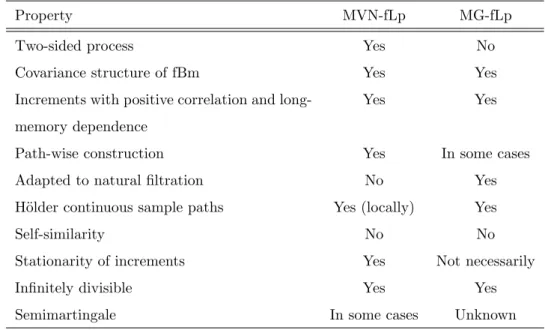
The following table allows a quick summary of the properties each fLp.

Property MVN-fLp MG-fLp

Two-sided process Yes No

Covariance structure of fBm Yes Yes

Increments with positive correlation and

long-memory dependence

Yes Yes

Path-wise construction Yes In some cases

Adapted to natural filtration No Yes

H¨older continuous sample paths Yes (locally) Yes

Self-similarity No No

Stationarity of increments Yes Not necessarily

Infinitely divisible Yes Yes

Semimartingale In some cases Unknown

Table 1: Comparing the MVN-fLp and the MG-fLp

The “two-sided” definition of the MVN-fLp happens to be quite important, for the same reasons given

to the integral representation of the fBm by Mandelbrot-van Ness. In this case, the simulation of the

process must lead to truncate the integral somewhere.

It is not hard to understand the reasons which made the Brownian motion be gradually substituted

(32)

3.4 Simulation 3 FRACTIONAL L ´EVY PROCESS

modelling are the following: the distribution of the increments of a L´evy process does not have to be the

Gaussian distribution, enabling, for example, a non-symmetric distribution with “heavier tails”, as well

as the possibility of admitting non-constant implied volatilities, and, finally, the sample paths of a L´evy

process may have “jumps” or discontinuities. All these upgrades assume all the other advantages of the

Brownian motion, besides it is more conform to empirical knowledge and more economically realistic. Yet,

the L´evy process is more analytically complicated to deal with, and for most cases there is no closed forms

solutions for important models based on L´evy processes, such as prices of options. The advance from

the Brownian motion to the L´evy process also rise problems in the economic functioning of the financial

models: the arbitrage issue may become a problem, and the hedging and completeness may not be possible

in most cases. Some may argue that, in some cases, the models are badly specified. But the advances

towards reality in modelling may also imply a badly and insufficient specification of the financial theory

as well.

Curiously, when comparing both previous fractional processes to the L´evy process, in some sense, it

does not seem to be an improvement, but actually a throwback. The trajectories of the fLp have no

longer jumps, and in some cases, they are differentiable on compacts (see Proposition 3.10), which is not

an expected trace on the movement of assets’ prices. But we gain a memory perspective which was not

contemplated within L´evy’s family.

Nevertheless, except for the excess of regularity of the fLp, the driving L´evy process impress the fLp

with more possibilities than the fBm. Actually the fLp is a family of processes, depending in the L´evy

process in which it relies. The fLp is not a Gaussian process (it is an immediate consequence of Proposition

3.10 in Tikanm¨aki and Mishura (2011)). And not all fLp have stationary increments. On the other hand,

the great advantage of the fLp, when compared with the fBm, is that it can be a semimartingale.

3.4 Simulation

In order to simulate the previous two fLp, we will present two main approaches.

3.4.1 Path-wise Riemann integral approach

In the present section, we propose a numerical method to simulate the previous fLp.

From Propositions 3.4 and 3.13, the problem of simulation of these processes is simply solved by a

numerical integration, method given a simulation of the driving L´evy process. This is a perfect fit for the

MVN-fLp, but not to the MG-fLp, since in this case, the Riemann integral representation is only available

(33)

3.4 Simulation 3 FRACTIONAL L ´EVY PROCESS

Simulation of the MNV-fLp Within this approach, by Proposition 3.4, the MNV-fLpXH

t is the result

of the following integral

Z

R

gt(s)ds, (3.10)

wheregt(s) =fH(t, s)L(s) for a givent∈R.

The simulation of X_tH, within this approach, is summarized by the simulation of the driving L´evy process and by the application of a numerical scheme to approximate an Riemann integral.

However, the functiongtis not continuous inRbut it is Lebesgue a.s. continuous. Let

. . . , τ−2, τ−1, τ1, τ2, . . .

be the instants of the jumps of the two-sided L´evy process.

So (3.10) can be written as

X

n

Z τn

τn₋1

gt(s)ds. (3.11)

If we choose, for instance, the composite trapezoidal scheme in m equally spaced partitions for the numerical approximation, each integral in (3.11) may be computed as

lim

δ→0+

Z τn−δ

τn₋1

gt(s)ds≈

(τn−ǫ)−τn−1

m

gt(τn−1)

2 +

m−1

X

k=1

gt

τn−1+

(τn−ǫ)−τn−1

m k

+gt(τn−ǫ) 2

!

,

with ǫ >0, where the ǫcorresponds to the approximation to the interval end where the function is not left-continuous. (Recall that the paths of L´evy process are right-continuous). The only point left is the

truncation of the integral (3.10), which can be picked a priori substituting R by the compact interval

[−k, k].

With this background, we can follow up the following steps in order to simulate the MNV-fLp.

Algorithm 3.1(Path-wise Riemann simulation of MVN-fLp). Using the trapezoidal rule for the integral’s approximation, for each t∈R,XH

t may be simulated by the following.

1. Fix a truncationk, a numbermof equally spaced partition intervals and truncationǫfor each interval;

2. Simulate the L´evy process Ls for s ∈ [−k, k], denote τ−∗n+1, . . . , τ−∗1, τ1∗, . . . , τn∗−1 to the simulated

jump instants, and call τ∗

−n=−k andτn∗=k, moreover τ0∗= 0;

3. For each interval[τ∗

i−1, τi∗−ǫ] define sk =τi∗−1+

τ∗

i−ǫ−τi∗₋1

m k, for k= 0,1, . . . , m and approximate

the integral over [τ∗

i−1, τi∗−ǫ]with

Ii:=

sn−s0

m

gt(s0)

2 +

m−1

X

k=1

gt(sk) + gt(sm)

2

!

;

F RANCISCO DEC ASTILHOM ONTEIROG

M

ESTRADO

M

ATEMÁTICA

F

INANCEIRA

TRABALHO FINAL DE MESTRADO

D

ISSERTAÇÃO

F

RACTIONAL

P

ROCESSES

:

A

N

A

PPLICATION TO

F

INANCE

F

RANCISCO DE

C

ASTILHO

M

ONTEIRO

G

IL

S

ERRANO

M

ESTRADO EM

M

ATEMÁTICA

F

INANCEIRA

TRABALHO FINAL DE MESTRADO

D

ISSERTAÇÃO

F

RACTIONAL

P

ROCESSES

:

A

N

A

PPLICATION TO

F

INANCE

F

RANCISCO DE

C

ASTILHO

M

ONTEIRO

G

IL

S

ERRANO

O

RIENTAÇÃO

:

J

OÃO

M

IGUEL

E

SPIGUINHA

G

UERRA

Contents

1

Introduction

2

Fractional Brownian Motion

2.1

Definition

2.2