UNIVERSIDADE NOVA DE LISBOA
Faculdade de Ciências e Tecnologia
Departamento de Ciências e Engenharia do Ambiente
EVALUATION OF THE POTENTIAL OF TRANSLOCATED
COMMON COCKLE FOR ECOLOGICAL RISK ASSESSMENT
STUDIES: BIOACCUMULATION AND BIOMARKERS TEST
Thesis submitted to the Faculdade de Ciências e Tecnologia to obtain the
Master’s degree in Environmental Engineering, profile in Ecological
Engineering
By: Jorge Lobo Arteaga
Under the guidance: Professor Doctor
Maria Helena Ferrão Ribeiro da
Costa
1
Acknowledgements
First of all, thanks to Professor Maria Helena Costa for support and time spent in guidance,
and special attention for Pedro Costa for teaching and giving me the support and
comprehension needed during all this time. Special thanks to Sandra Caeiro for the
cooperation and availability. Thanks to Mr. Manuel Ribeiro for the provision of cockles.
Special thanks have to be given to the Instituto Nacional dos Recursos Biológicos
(IPIMAR_INRB) for the collaboration in this work, particularly to Marta Martins. And most
of all, I want to thank my friends and family for their support, encourage, advice, and for
always being there.
The present research was approved by the Portuguese Science and Technology Foundation
(FCT) and POCTI (Programa Operacional Ciência, Tecnologia e Inovação, research project
ref. POCTI/AMB 57281/104) and financed by FEDER (European Fund for regional
Sumário
A contaminação sedimentar é um factor de grande preocupação em estuários e outras massas de águas costeiras confinadas, muitas vezes submetidas a fontes antropogénicas de poluição. Com o objectivo de investigar os efeitos e respostas do berbigão comum (Cerastoderma edule) aos contaminantes no sedimento e avaliar o potencial da espécie como organismo
indicador, o bivalve foi submetido a um ensaio de translocação com sedimentos colectados de diferentes locais do estuário do Sado (Portugal). Os berbigões foram recolhidos num local de maricultura do estuário do Sado (Portugal), identificado como local D, e foram expostos em ensaios de laboratório semi-estáticos, a sedimentos colectados noutros três locais do estuário (A, B e C) que revelaram diferentes níveis de metais, contaminantes orgânicos e distintas propriedades fisico-químicas, correspondendo a condições que vão desde ausência de impacte a impacte moderado quando comparados com os valores-guia de qualidade sedimentar disponíveis. Os bivalves foram analisados para bioacumulação de metais (Ni, Cu, Zn, As, Cd e Pb) e contaminantes orgânicos (PAHs, PCBs e DDTs). Empregaram-se dois conjuntos de biomarcadores para avaliar a toxicidade potencial: indução de metalotioninas (MT) e histopathologia da glândula digestiva. Estimaram-se o factor de bioacumulação (BAF) e o factor de acumulação biota-sedimento (BSAF) como índices ecológicos de exposição a metais e compostos orgânicos. Encontraram-se correlações significativas e positivas entre BSAF e MT para PHAs, e entre cada factor (BAF e BSAF) e MT para o Cd. Encontraram-se alterações histopatológicas nos berbigões expostos a todos os sedimentos para onde foram translocados, houve uma degradação da integridade da glândula digestiva principalmente nos organismos do sedimento B e C e no dia 28 do sedimento A. Os resultados permitiriam concluir que C. edule responde a sedimentos contaminados e é capaz de regular e eliminar
3
Abstract
Sediment–bound contamination is a major concern factor in estuaries and other confined coastal water bodies, frequently subjected to anthropogenic sources of pollution. In order to investigate the effects and responses of the common cockle (Cerastoderma edule, L. 1558,
Bivalvia: Cardiidae) to sediment contaminants and to assess the species’ potential as an indicator organism, the bivalve was subjected to a laboratorial translocation assay with sediments collected from distinct sites of the Sado Estuary (Portugal). Cockles were collected from a mariculture site of the Sado estuary (Portugal), herewith identified as site A, and exposed through 28–day, semi–static laboratorial essays, to sediments collected from three other sites (B, C and D) of the estuary that revealed different levels of metals, organic contaminants and physico–chemical properties and that ranged from globally unimpacted to moderately impacted levels when compared to available sediment quality guidelines. The animals were surveyed for bioaccumulation of metals (Ni, Cu, Zn, As, Cd and Pb) and organic contaminants (PAHs, PCBs and DDTs). Two sets of potential biomarkers were employed to assess toxicity: whole–body metallothionein (MT) induction and digestive gland histopathology. The bioaccumulation factor (BAF) and the biota-to-soil accumulation factor (BSAF) were estimated as ecological indices of exposure to metals and organic compounds. Significant positive correlations between BSAF and MT were found for PHAs, and between each factor (BSAF and BAF) and MT were found for Cd. Histopathological alterations were found in cockles exposed to all sediments where they were translocated. The digestive gland integrity was found to be especially compromised in cockles from sediment B and C and at day 28 from sediment A. Results allowed concluding that C. edule responds to sediment–
Symbology
T0 sampling day 0
T14 sampling day 14
T28 sampling day 28
ww wet weight
dw sediment dry weight
Eh sediment redox potential
TOM total organic matter
MT metallothionein
Ni nickel
Cu copper
Zn zinc
Cd cadmium
Pb lead
As metalloid arsenic
PAH polycyclic aromatic hydrocarbon
PCB polychlorinated biphenyl
DDT dichloro-diphenyl-trichloroethane
tPAH total PAH (sum of all individual PAHs)
tPCB total PCB (sum of all congeners)
tDDT total DDT (pp'DDD+pp'DDD+pp'DDT)
DDD 1,1-dichloro-2,2-bis(ρ-chlorophenyl)ethane
DDE 1,1-dichloro-2,2-bis (ρ-chlorophenyl)ethylene
DDT 1,1,1-trichloro2,2-bis (ρ-chlorophenyl)ethane
GC–MS gas chromatography–mass spectrometry
ICP-MS inductive coupled plasma atomic emission spectrometry
TEL threshold effects level
PEL probable effects level
PEL-Q PEL quotient
SQG-Q sediment quality guideline quotient indice
BAF bioaccumulation factor
5
Index
1 Introduction ... 9
2 Materials and methods ... 14
2.1 Experimental assay ... 14
2.2 Sediments analyses... 16
2.2.1 Physico chemical characterization ... 16
2.2.2 Contaminant determination ... 16
2.3 Organisms analyses ... 18
2.3.1 Bioaccumulation ... 18
2.3.2 Metallothionein induction ... 19
2.3.3 Histopathology ... 19
2.4 Bioaccumulation (BAF) and biota-sediment accumulation (BSAF)
factors... 20
2.5 Statistical analysis ... 21
3 Results... 22
3.1 Physical characterization of sediments... 22
3.2 Contaminants in sediments... 23
3.3 Bioaccumulation in C. edule... 26
3.4 BAFs and BSAFs... 28
3.5 Histopathology ... 30
4 Discussion ... 34
References ... 40
Index Figures
Fig. 1 - Map of the study area...15 Fig. 2 - Linear relation between FF and TOM for all sediments tested. ...22 Fig. 3 - Metal concentrations of sediments from sites D, A, B and C and TEL and PEL for
each metal and metalloid. ...24 Fig. 4 - Concentrations of 3- ring PAHs of sediments from sites D, A, B and C and TEL and
PEL for each compound. ...25 Fig. 5 - Concentrations of 4- and 5- ring PAHs of sediments from sites D, A, B and C and
TEL and PEL for each compound. ...25 Fig. 6 - tPCB and PAH (pp’DDD, pp’DDE and pp’DDT) concentrations of sediments from
sites D, A, B and C and TEL and PEL for each compound. ...26 Fig. 7 - Concentration of metallothioneins in C. edule after 14 and 28 days of exposure to all
sediments. ...26 Fig. 8 - Bioaccumulation of Cu, As, Cd and Pb after 14 and 28 days of exposure to all
sediments. ...27 Fig. 9 - Bioaccumulation of Ni and Zn after 14 and 28 days of exposure to all sediments. ....27 Fig. 10 - Bioaccumulation of organic contaminants after 14 and 28 days of exposure to all
sediments. ...28 Fig. 11 – MT (mg.g-1 whole soft tissue dry weight) and BAFs and BSAFs for Cd after 14 and
28 days of exposure to all sediments...29 Fig. 12 - MT (mg.g-1 whole soft tissue dry weight) and BAFs and BSAFs for tPAHs after 14
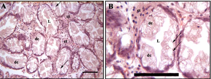
and 28 days of exposure to all sediments. ...29 Fig. 13 - Histological sections stained with haematoxylin and eosin of digestive gland of C.
edule.. ...30
Fig. 14 - Histological sections stained with haematoxylin and eosin of digestive gland of C. edule. ...31
Fig. 15 - Histological sections stained with haematoxylin and eosin of digestive gland of C. edule. ...32
Fig. 16 - Histological sections stained with haematoxylin and eosin of digestive gland of C. edule. ...33
Fig. 17 – Diversity of organisms found within C. edule in systems of acclimatization after a
7
Index Tables
Table 1 - Bivalve species in which Biomarkers have been shown to be induced by
Index Annexes
Annex I - Metal and organic concentrations of sediments from sites D, A, B and C. ...47 Annex II - Metallothionein and bioaccumulation of metal and organic contaminants in
9
1
Introduction
Marine bivalve molluscs are mainly filter-feeding organisms which due to their sedentary
lifestyle, are characterised by their very high capability to bioaccumulate chemical substances
dissolved in the water or bound to suspended particles (Machreki-Ajmi et al. 2008; Solé et al.
2009). These substances can be organic compounds and trace metals (essential or not), both
with potential to cause toxic effects. Bivalve filter-feeders are therefore considered good
bioindicators for the assessment of environmental quality (Cajaraville et al. 2000; Hédouin et
al. 2007). The assessment of polluted environments based only in chemical analyses is
difficult, particularly the assessment of polluted sediments due to the complex nature of the
sediment matrix and the potential for exposure of aquatic organisms to in-place contaminants
via several routes (Del Valls et al. 1998). The use of biomarkers has been considered to be
viable measures of impact of toxicity (Huggett et al. 1992; Peakall and Shugart 1993). In
recent years, biomarkers that may provide information on the effects of xenobiotics in
organisms have received considerable interest and many of them have been validated in
bivalves (Geret et al. 2003; Bergayou et al. 2009). Mussels and oysters are the marine
bivalves most used in pollution monitoring. However, other species have been intensively
studied because of their importance for human consumption or their close contact with
sediment (Amiard et al. 2006). Some of these species have been widely employed in toxicity
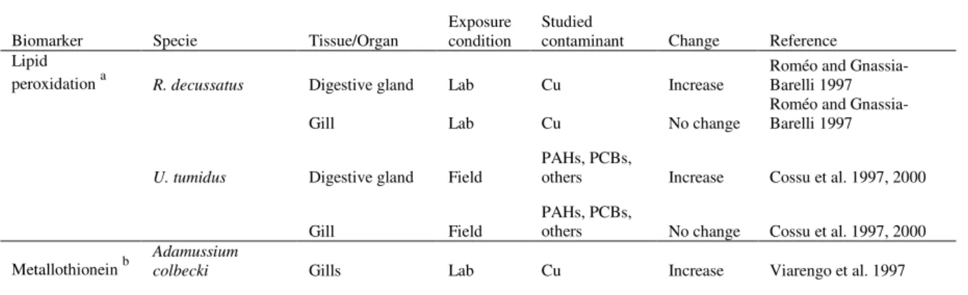
test and biomarker techniques have already been validated (Table 1).
Table 1 - Bivalve species in which Biomarkers have been shown to be induced by contaminant exposure.
Biomarker Specie Tissue/Organ
Exposure condition
Studied
contaminant Change Reference Lipid
peroxidation a R. decussatus Digestive gland Lab Cu Increase
Roméo and Gnassia-Barelli 1997
Gill Lab Cu No change
Roméo and Gnassia-Barelli 1997
U. tumidus Digestive gland Field
PAHs, PCBs,
others Increase Cossu et al. 1997, 2000
Gill Field
PAHs, PCBs,
others No change Cossu et al. 1997, 2000
Biomarker Specie Tissue/Organ
Exposure condition
Studied
contaminant Change Reference
Anadara granosa Blood Lab Cd Increase Chan et al. 2002
Anodonta anatina Kidney Lab Cd Increase Streit and Winter 1993
Anodonta cygnea Whole soft tissue Lab Cu No change Tallandini et al. 1986
Whole soft tissue Lab Zn No change Tallandini et al. 1986
Anodonta grandis Gills Field Cd Increase
Couillard et al. 1993, Giguère et al. 2003 Digestive gland Field Cd Increase Couillard et al. 1993
Remaining soft
tissue Field Cd Increase Couillard et al. 1993
(Anodonta)
Pyganodon grandis Whole soft tissue Field Cd Increase Couillard et al. 1995a
Gills Field Cd Increase Wang et al. 1999
Corbicula fluminea
Gill, mantle and
adductor muscle Lab Cd Increase Doherty et al. 1988 Visceral mass Lab Cd Increase Doherty et al. 1988 Whole soft tissue Field Cd Increase Baudrimont et al. 1999 Whole soft tissue Field Zn Increase Baudrimont et al. 1999
Macoma balthica Whole soft tissue Lab Cu Increase Johansson et al. 1986
Whole soft tissue Field Cu Increase Ag Johansson et al. 1986 Whole soft tissue Field Zn Increase Ag Johansson et al. 1986 Whole soft tissue Field Ag Increase Ag Johansson et al. 1986 Whole soft tissue Lab Cd Increase Bordin et al. 1994, 1997 Whole soft tissue Lab Cu Increase Bordin et al. 1994, 1997 Whole soft tissue Lab Zn Increase Bordin et al. 1994, 1997 Whole soft tissue Field Cd Increase Bordin et al. 1997 Whole soft tissue Field Cu Increase Bordin et al. 1997 Whole soft tissue Field Zn Increase Bordin et al. 1997 Whole soft tissue Lab Cd Increase Mouneyrac et al. 2000 Whole soft tissue Lab Ag Increase Mouneyrac et al. 2000 Whole soft tissue Lab Hg Increase Mouneyrac et al. 2000 Whole soft tissue Field Cu Increase Bray et al. 1983 Whole soft tissue Field Ag Increase Bray et al. 1983 Mercenaria
mercenaria Kidneys Lab Cd Increase Robinson et al. 1985
Mizuhopecten
yessoensis Gills Lab Cd Increase Evtushenko et al. 1986
Hepatopancreas Lab Cd Increase Evtushenko et al. 1986
Protothaca straminea
Viscera and
Kidney Lab Cd Increase Roesijadi 1980
Viscera and
Kidney Lab Cu Increase Roesijadi 1980
Viscera and
Kidney Lab Zn Increase Roesijadi 1980
Rangia cuneata Whole soft tissue Field Cu Increase Bray et al. 1983
Whole soft tissue Field Ag Increase Bray et al. 1983 Ruditapes
decussatus Whole soft tissue Lab Cd Increase Bebianno et al. 1993
Digestive gland Lab Cd Increase Bebianno et al. 1993
Gills Lab Cd Increase Bebianno et al. 1993
Digestive gland Lab Cu Increase
Hamza-Chaffai et al. 1998
Gills Lab Cu Increase
Roméo and Gnassia-Barelli 1995
Gills Lab Cd Increase
Bebianno and Serafim 1998
11
Biomarker Specie Tissue/Organ
Exposure condition
Studied
contaminant Change Reference Digestive gland Lab Cd Increase Ng and Wang 2004 Digestive gland Lab Zn No change Ng and Wang 2004 Digestive gland Lab Ag Increase Ng and Wang 2004 Whole soft tissue Lab Cd Increase Ishiguro et al. 1982 Scapharca
inoequivalis Lab Cd Increase Serra et al. 1995
AchE Scrobicularia plana Digestive gland Field
metals/organics
(PCB, PAH) Change Solé et al. 2009 a Adapted from Livingstone 2001
b Adapted from Amiard et al. 2006
The common cockle (Cerastoderma edule, Bivalvia: Cardiidae) is a filter-feeding bivalve
common in the North Sea and north-east Atlantic, being widely distributed from north-east
Norway to West Africa. It lives buried in the upper few centimetres of the sediment,
frequently forming high populational densities, in marine and estuarine environments. High
inter-individual variability of reproduction stage, parasite load, metallothionein (MT)
concentration, etc. is generally observed in C. edule populations (Baudrimont et al. 2006). It is
highly tolerant to environmental variations of physico-chemical parameters such as sediment
grain size and salinity, and may thus be employed as an indicator organism along an estuarine
gradient. In Sado estuary, i.e. this cockle colonizes all intertidal sediments, from the sand
beach of Tróia Peninsula close to the estuarine mouth to the mudflats in the channel of Águas
de Moura. C. edule has been tested in recent studies (Jung et al. 2006) but despite its
characteristics, there are very few ecotoxicological studies with this bivalve.
The response to sediment–bound contamination and the capacity to regulate and eliminate
both organic and metallic contaminants are reflected in biomarkers. Biomarkers are defined as
indicators of normal biological processes, pathogenic processes or pharmacological responses
to a therapeutic intervention (Biomarkers Definitions Working Group 2001) Biomarkers can
be indicators of either exposure or effects. Biomarkers of exposure indicate that exposure to a
chemical or class of chemical has occurred, but do not provide knowledge of toxic effects at
the level of the organisms, and the biomarkers of effect reflect a deteriorating condition
employed. MT is a protein involved in metal (essential or not) accumulation and elimination
strategies and, in many bivalves MT response has been found revealing higher sensitivity with
increase of pollution (Marie et al. 2006; Serafim and Bebianno 2009). However, metals are
not the only factor in the MT induction, also other factors can interfere: in C. edule the
possible impact of the period of reproduction, the infection of digenean parasites as well as
other factors related with the metabolic state of each specimen supposed to be important
contributors to fluctuations in MT concentration (Baudrimont et al. 2006). Most of the
histopathological lesions could be related to environmental stressors, as soft-tissue
concentrations of contaminants (Gold-Bouchot et al. 1995). Gills and digestive gland in
molluscs appear to be good survey organs for pollution studies (Gold-Bouchot et al. 1995;
Syasina et al. 1997; Zaldibar et al. 2007, 2008), but the histopathology in C. edule has
received little or no focus at all.
The Sado estuary, located on the west coast, is the second largest in Portugal with an area of
approximately 24,000 ha. The estuary comprises the Northern and the Southern Channels,
partially separated by intertidal sandbanks. Water exchange is conducted mainly through the
Southern Channel, which reaches a depth of 25 meters, whereas the maximal depth of the
Northern Channel is generally 10 meters. Most of the estuary is classified as a natural reserve,
with a weighty ecological and landscape value. The region equally plays an important role for
the leisure and recreation, and therefore, is important in the local and national economy. The
city of Setúbal located in the North edge of Sado estuary, has a large resident population and
an important heavy-industry in the adjacent area. The estuary is an important fishing area and
many aquaculture facilities have been settled here along the past few years. The southernmost
section of the estuary is mainly characterized by an important tourism-based economy. The
major sources of anthropogenic contaminant input are mainly the pyrite mines in the river
basin, the industries that involving pulp and paper, pesticides, fertilizers, yeast, food and
13 from extensive agriculture grounds located upstream. The results of previous studies indicate
that anthropogenic sources play a major role on the elemental composition of the Sado
estuarine sediments (Cortesão and Vale 1995) and, this estuary has a low contamination level
with some local hotspots and a moderate potential for observing adverse biological effects
(Caeiro et al. 2005).
Translocation of bivalves between areas with different levels of water and sediment
contamination has long been employed for standard biomonitoring of aquatic ecosystems.
These procedures have been proved to provide valuable information on the molluscs’
responses and defences to contamination, with especial respect to the kinetics of xenobiotic
uptake and elimination (see De Kock and Kramer 1994 for a thorough review).
The present work intends to recreate a translocation assay with C. edule, under controlled
laboratorial conditions in order to determine the species’ potential as an indicator organism
for contaminated estuarine sediments and to assess the effects and responses of exposure to
2
Materials and methods
2.1
Experimental assay
The sediments were collected from four different sites (designated as sites A, B, C and D) of
the Sado estuary (Fig. 1) on November 2006, selected by their different levels of metallic and
organic contamination. Site A is located near an environmentally protected area, the Sado
estuary Natural Reserve, and is the most distant from sources of direct contamination. Due to
its location in the south channel of estuary, this site has a greater influence of oceanic
hydrodynamics and a lower residence time than the others. Site B is located near the port of
Setúbal and site C in the industrial zone near factories for the production of fertilizers,
pesticides and others (such as paper mills, thermoelectric, shipyards, etc), having been
identified as potentially contaminated. They are both located in the North Channel, an area of
low hydrodynamics which facilitate the retention of contaminants and fine particles of
sediment coming from the upper estuary. Site D, located near aquaculture and small-scale
fishery grounds consist of a lower hydrodynamics, relatively confined, area. Site D is the only
one located in the intertidal zone, and the other sites (A, B and C) are located in the subtidal
15 Fig. 1 - Map of the study area.
Cockles [28 ± 1.6 mm shell length, 8.0 ± 1.4 g wet weight (ww)] were collected on November
2006 from site D of the Sado estuary and acclimatized to test conditions (temperature of 18ºC
and salinity of 34) in clean sand and seawater for 48h. The bivalves were exposed to the
sediments (A, B and C) for 28 days through a static arrangement of bioassays (performed in
duplicate). Each replicate consisted of a tank (24x11x39 cm) in which were allocated 2 L of
sediment and 5 L of clean seawater. Forty animals were distributed per tank, exposed to
continuous aeration and fed with commercial fish food (Avipar Lda., Portugal) during assay.
Each week, 50% of the seawater was changed and the following parameters monitored:
salinity, dissolved oxygen, ammonia, pH and temperature. The animals were collected and
sacrificed for analysis on day 0 (T0), 14 (T14) and 28 (T28) in order to determine
histopathological alterations of the digestive gland. For each test and sampling time, 20
individuals were used to determine the organic contaminants, 10 individuals to determine the
metals and metallothioneins and 10 to examine the histopathology. Animals collected at T0
consisted of 15 individuals collected directly from the acclimatization tanks.
2.2
Sediments analyses
2.2.1 Physico chemical characterization
Sediment redox potential (Eh) was measured immediately after collection, using an Orion
model 20A meter with a H3131 Ag/AgCl reference electrode (Orion Research Inc., USA).
For the analysis of organic matter, the sediment was previously dried in stove at 60-80 °C in a
and then combusted in oven at 500 ± 25 °C for 4 hours. The content of organic matter
(extrapolated from total combustible carbon, TOM) is given in percent (%) sediment dry
weight (dw). Fine fraction (particle size < 63 µm) was determined by sieving after treating the
samples with hydrogen peroxide and disaggregation with pyrophosphate.
2.2.2 Contaminant determination
The sediments were analysed for the metals nickel (Ni), copper (Cu), zinc (Zn), cadmium
(Cd) and lead (Pb), and the metalloid arsenic (As). Sediment samples (≈100 mg dw) were
mineralized completely with 6 cm3 of HF (40%) and 1 cm3 of Aqua Regia (HCl-36%: HNO3
-60%; 3:1) in closed Teflon vials in a water bath at 100 °C during 1 h. Contents were
evaporated to near dryness redissolved in HNO3 and Milli-Q water, heated for 20 min at 75
17 concentrations were determined in the same samples but in separate runs using a quadropole
ICP-MS (Inductive coupled plasma atomic emission spectrometry) (Thermo Elemental,
Xseries, USA) equipped with a Peltier Impact bead spray chamber and a concentric Meinhard
nebulizer. MESS-2 (NRC, Canada), PACS-2 (NRC, Canada) and MAG-1 (USGS, USA) were
the references materials used to validate the procedure and were found within the certified
range. Results are given in mg kg-1 sediment dw.
The determination of PAHs (polycyclic aromatic hydrocarbons) was performed on a GCQ
Trace Finnigan gas chromatography–mass spectrometry (GC-MS) system with a 30 m · 0.25
mm · 0.25 lm film thickness DB-5 MS column (Argilent, USA) in selected ion mode (SIM)
(Martins et al. 2008). Seventeeen three- to six-ring PAHs were quantified. For PCB
(polychlorinated biphenyls) and DDT (dichloro-diphenyl-trichloroethane) analysis, dry
sediment samples and glass-fibre filters with suspended particulate matter were Soxhlet
extracted with n-hexane for 16 h. The extracts were cleaned up with Florisil and sulfuric acid
(Ferreira et al. 2003). Eighteen PCB congeners and pp’DDD, pp’DDE and pp’DDT as total
DDT were analysed. The SMR 1941b reference sediment (NIST, USA) was used to validate
of the analysis and were found within the certified range. The detection limit was 0.01 ng.g-1.
All concentrations are expressed in ng g−1.sediment dw.
The PEL quotient (PEL-Q) was calculated to evaluate the impact potential for observing
adverse biological effects of the tested sediments. This quotient is based on the published
guideline values for coastal waters, namely the threshold effects level (TEL) and the probable
effects level (PEL) (MacDonald et al. 1996). These guidelines have been largely used in
estuarine sediment ecological risk assessment studies. This index was calculated for all
contaminants of each sediment as given by the formula (Long and MacDonald 1998):
---
Note: the quantification of organic conaminants in sediments (PAHs, PCBs and DDTs) by GC-MS was performed by the Instituto Nacional dos Recursos Biológicos
PEL−Qi= Ci
PEL [1]
where PEL is the guideline value for the contaminant i and Ci the measured concentration of
the contaminant in the surveyed sediment. The sediment quality guideline quotient indice
(SQG-Q) was calculated to compare the four sites impacted by mixtures as described by Long
and MacDonald (1998):
[2]
where PEL-Qi is the indice deriving from [1] for the contaminant i and n the number of
contaminants under analysis. Stations were scored according to their overall potential of
observing adverse biological effects, as proposed by MacDonald et al. (2004): SQG-Q < 0.1 -
unimpacted; 0.1 ≤ SQG-Q < 1 - moderately impacted; SQG ≥ 1 - highly impacted.
2.3
Organism analysis
2.3.1 Bioaccumulation
For the analysis of metals, whole-body individual samples were dried (0.025 ± 0.003 g dw) in
borosilicate, lead free, glass vials at 60 ºC during 5 days and then transferred to Teflon vessels
adding 5 ml nitric acid (65%) to digest for 24 hours at room temperature. They were placed in
a water bath at 95 ºC during 4 hours, then 1 ml hydrogen peroxide (30% v/v) was added and
Teflons were placed in the water bath for another hour (Clesceri et al. 1999). Finally, the
samples are stored in HDPE plastic bottles (25 ml) after elution with Mili-Q water and were
kept at 4 ºC until reading. The quantification of the concentrations of metals (Ni, Cu, Zn, Cd
SQG−Q=
−Qi
i=1
n
∑
19 and Pb) and metalloid (As) was determined using ICP-MS. The organic contaminants were
determined in the same sample by GC-MS after soxhlet extraction (3- to 6 ring PAH, 18 PCB
congeners plus pp’DDD, pp’DDE and pp’DDT as total DDT). Quantification was carried out
similarly to the procedure described in the sediments, adapted to biological tissue (Martins et
al. 2008).
2.3.2 Metallothionein induction
Metallothionein induction was determined by quantification of thiols in whole soft tissue
samples according to Costa et al. (2008). In brief: samples were homogenized in Tris-HCl
0.02 M buffer (pH 8.6). Homogenates were centrifuged at 17,000 rpm at 4 ° C for one hour.
The supernatant was heated in a water bath at 80 °C for 10 minutes to destroy the proteins
with less thermal stability, and were centrifuged as previously described. Finally, the
metallothioneins were quantified from heat-treated cytosols by differential-pulse
polarography with a static mercury-drop electrode (DPP-SMDE) using a 693 VA processor
and a 694 VA stand (Metrohm, Herisau, Switzerland). In absence of a commercial form of
bivalve MT, Rabbit MT isoforms I & II (Sigma, St Louis, MO, USA) was used for the
standard addition method.
2.3.3 Histopathology
Cockles were fixed in Bouin-Holland’s solution (27% formaldehyde, 7% acetic acid, and
picric acid until saturation) for approximately 48 hours at room temperature. Afterwards, the
samples were washed with water for 24 hours to remove the excess picric acid, dehydrated in
---
Note: the quantification of organic conaminants in organisms (PAHs, PCBs and DDTs) by GC-MS was performed by the Instituto Nacional dos Recursos Biológicos
a progressive series of ethanol, an intermediate embedding with xylene (≈ 100%) was carried
out. Samples were then embedded in paraffin for about 12 hours. The blocks were cut in
sections of 5 µm and then stained with haematoxylin and eosin (H & E) (Martoja and Martoja
1967) and mounted with DPX resin (BDH).
2.4
Bioaccumulation and biota-sediment accumulation factors
The bioaccumulation factor (BAF) and the biota-to-sediment accumulation factor (BSAF)
were measured regarding the metals (Ni, Cu, Zn, Cd and Pb), metalloid (As ) and organic
contaminants (PAHs, PCBs and DDTs). The BAF was calculated after 14 and 28 days of
exposure according to the formula (Lee 1992):
s o C C
BAF= [3]
The BSAF after 14 and 28 of exposure = BAF normalized to the organic carbon content in the
sediment (adapted from formula of USEPA 1995):
[4]
where Co was contaminant concentration in organism expressed in mg.kg-1 dry weight of
tissue, Cs was contaminant concentration in sediment expressed in mg.kg-1 dry weight of
sediment, and TOM was expressed in % Total Organic Matter of sediment on a dry weight
basis.
BSAF= Co Cs
21
2.5
Statistical analysis
The non-parametric tests Kruskall-Wallis H and Mann-Whitney U were employed to
assess global and pairwise statistical differences, respectively. The Chi-square predicted x
observed test was applied to assess significant differences between the concentrations of
organic contaminants (in sediment and bioaccumulation) of all tests and sampling points. The
non-parametric Spearman’s Rank Order Correlation ρ statistic was used to assess the
correlation between BAFs/BSAFs and metallothioneins. A significance level of 5% was set
for all analyses. All the statistical results were obtained using Statistical Package for Social
3
Results
The values obtained of the parameters monitored each week were under standard conditions.
Values were the following: salinity = 34 ± 1, dissolved oxygen = 42 ± 2 %, ammonia < 0,5
mg L-1, pH = 7.8 ± 0.1, and temperature = 18 ± 1 ºC.
3.1
Physical characterization of sediments
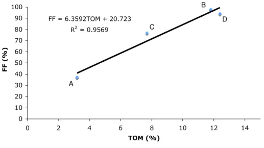
There is a linear relation between FF and TOM content in sediments from the 4 sites (Fig. 2).
Fig. 2 - Linear relation between FF and TOM for all sediments tested.
The sediment A has less FF and TOM. The other sediments have high FF and TOM, the grain
size of B and D is almost entirely FF (97,9 and 94,1 % respectively) and have a high organic
matter content (11,8 and 12,4 % respectively).
Redox potential is negative for all sites, being C the most reduced sediment. D is the only
intertidal sediment and it is the less reduced (Table 2).
B
D
A
23 Table 2 - Characterization of sediments from sites D, A, B, and C.
Site FFa (%) TOMb (%) Ehc (mV)
D 94.1 12.4 -187
A 37.3 3.2 -233
B 97.9 11.8 -290
C 76.8 7.7 -316
a Particle size < 63 µm b Total organic matter c Redox Potential
3.2
Contaminants in sediments
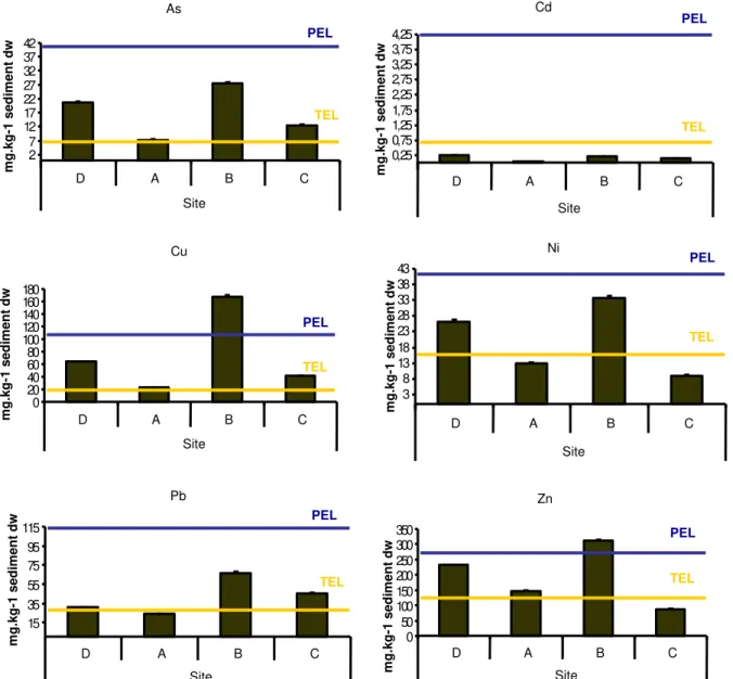
The results of the metal and organic concentrations on sediments from the 4 sites are
presented in Annex I. The sediments B and D present higher concentrations of metals and
metalloid (As), with values above TEL for all metals and metalloid except Cd, highlighting
concentrations of Zn and Cu above PEL in sediment B. As, Cu and Zn present values above
TEL on sediment A and As, Cu and Pb present values above TEL on sediment C (Fig. 3).
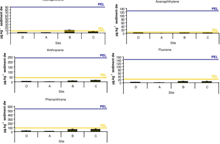
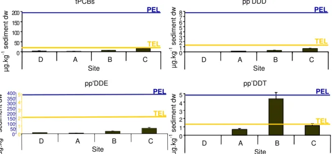
Values of tPAHs obtained decreased in the following order on sediments: C>B>D>>>A.
Concentrations of 4- and 5-ring PAHs were higher on all sediments. Values above TEL were
not found in the sediment A, and only a few compounds of 3-, 4- and 5-ring PAHs had
concentrations above TEL on sediments B, C and D (Fig. 4 and 5). Values of tPCBs obtained,
decreased in the following order on sediments: C>>B>D>A, with any value above TEL (Fig.
6). The levels of the organic contaminants analysed were irrelevant in the sediment A
compared with other sediments; PCB-26 (tri-chlorinated) was the congener with higher
concentration on sediment D; penta-, hexa- and hepta-chlorinated were the higher
with the highest concentration on the sediment C were PCB-101 and PCB- 118
(penta-chlorinated), and PCB-138, PCB-151 and PCB-153. The values of tDDTs obtained decreased
in the following order on sediments: B>C>A>D. Sediment D presents very low
concentrations of tDDTs, pp’DDE was the only above detection limit. pp’DDT were the
forms with the highest concentrations on sediments A, B and C, particularly on sediment B
(Fig. 6), being the major metabolite of tDDTs. Value obtained of SQG-Q for the 4 sediments
follow the sequence (from worst to best sediment quality): B>D>C>A. Due to the weight of
SQG-Q is mainly metallic for all sediments, SQG-Q discriminated calculated for metals
follow the same sequence as for the total, but those calculated for organics: B>C>D>A.
Fig. 3 - Metal concentrations of sediments from sites D, A, B and C and TEL and PEL for each metal and metalloid.
As 2 7 1 2 1 7 2 2 2 7 3 2 3 7 4 2
D A B C
Site m g .k g -1 s e d im e n t d w TEL PEL Cd
0 , 2 5 0 , 7 5 1 , 2 5 1 , 7 5 2 , 2 5 2 , 7 5 3 , 2 5 3 , 7 5 4 , 2 5
D A B C
Site m g .k g -1 s e d im e n t d w TEL PEL Ni 3 8 1 3 1 8 2 3 2 8 3 3 3 8 4 3
D A B C
Site m g .k g -1 s e d im e n t d w TEL PEL Zn 0 5 0 1 0 0 1 5 0 2 0 0 2 5 0 3 0 0 3 5 0
D A B C
Site m g .k g -1 s e d im e n t d w TEL PEL Cu 0 2 0 4 0 6 0 8 0 1 0 0 1 2 0 1 4 0 1 6 0 1 8 0
D A B C
Site m g .k g -1 s e d im e n t d w TEL PEL Pb 1 5 3 5 5 5 7 5 9 5 1 1 5
D A B C
25 Fig. 4 - Concentrations of 3- ring PAHs of sediments from sites D, A, B and C and TEL and PEL for each compound.
Fig. 5 - Concentrations of 4- and 5- ring PAHs of sediments from sites D, A, B and C and TEL and PEL for each compound.
Acenaphthene 0 10 20 30 40 50 60 70 80 90
D A B C
Site µ g .k g -1 s e d im e n t d w TEL PEL Acenaphthylene 0 20 40 60 80 100 120 140
D A B C
Site µ g .k g -1 s e d im e n t d w TEL PEL Anthracene 0 50 100 150 200 250
D A B C
Site µ g .k g -1 s e d im e n t d w TEL PEL Fluorene 0 20 40 60 80 100 120 140 160
D A B C
Site µ g .k g -1 s e d im e n t d w TEL PEL Phenanthrene 0 100 200 300 400 500 600
D A B C
Site µ g .k g -1 s e d im e n t d w TEL PEL Benz(a)anthracene 0 100 200 300 400 500 600 700
D A B C
Site µ g .k g -1 s e d im e n t d w TEL PEL Chrysene 0 100 200 300 400 500 600 700 800 900
D A B C
Site µ g .k g -1 s e d im e n t d w TEL PEL Fluoranthene 0 200 400 600 800 1000 1200 1400 1600
D A B C
Site µ g .k g -1 s e d im e n t d w TEL PEL Pyrene 0 200 400 600 800 1000 1200 1400
D A B C
Site µ g .k g -1 s e d im e n t d w TEL PEL Benzo(a)pyrene 0 100 200 300 400 500 600 700 800
D A B C
Site µ g .k g -1 s e d im e n t d w TEL PEL Dibenzo(a,h)anthracene 0 20 40 60 80 100 120 140
D A B C
Fig. 6 - tPCB and PAH (pp’DDD, pp’DDE and pp’DDT) concentrations of sediments from sites D, A, B and C and TEL and PEL for each compound.
3.3
Bioaccumulation and metallothioneins in C. edule
The results of metallothioneins and bioaccumulation in C. edule are present in Annex II.
Significant decrease of metallothioneins over time stands out in organisms of the sediment C
(Fig. 7).
Fig. 7 - Concentration of metallothioneins in C. edule after 14 and 28 days of exposure to all
sediments.
* indicates significant differences (ρ<0,05) between tests and D (Mann–Whitney U test) MT 0 1 2 3 4 5 6
D A B C A B C
T0 T14 T28
S ite and time of sam pling
m g .k g -1
*
*
pp’DDD 0 1 2 3 4 5 6 7 8D A B C
Site TEL PEL tPCBs 0 50 100 150 200
D A B C
Site TEL PEL pp'DDE 0 1 2 3 4 5
D A B C
Site 0 50 100 150 200 250 300 350 400 TEL PEL pp’DDT 0 1 2 3 4 5
D A B C
Site
µ
g
.k
g
-1 s
e d im e n t d w TEL PEL µ g .k g
-1 s
e d im e n t d w µ g .k g
-1 s
e d im e n t d w µ g .k g
-1 s
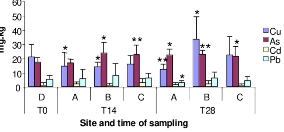
27 There is a great variability of the bioaccumulation of metals in each individual and over time.
Main rates of bioaccumulation are found in organisms of sediment B, with statistically
significant differences in As (p < 0,01), Pb (p < 0,05) and Zn (p < 0,01) (Fig. 8 and 9).
0 10 20 30 40 50 60
D A B C A B C
T0 T14 T28
Site and time of sampling
Cu As Cd Pb m g .k g -1
Fig. 8 - Bioaccumulation of Cu, As, Cd and Pb after 14 and 28 days of exposure to all sediments.
* and ** indicate significant differences (p < 0,05 and p < 0,01, respectively) between tests and D (Mann–Whitney U test)
0 50 100 150 200 250
D A B C A B C
T0 T14 T28
Site and time of sampling
m g .k g -1 Ni Zn
Fig. 9 - Bioaccumulation of Ni and Zn after 14 and 28 days of exposure to all sediments. * and ** indicate significant differences (p < 0,05 and p < 0,01, respectively) between tests and D (Mann–Whitney U test)
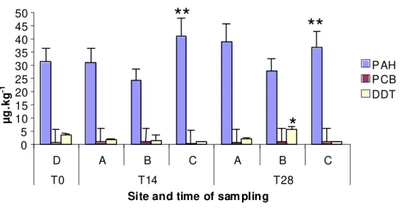
3- and 4-ring were the major compounds identified in PAHs, and they were bioaccumulated in
sediment C with statistically significant differences (p < 0,01). PCBs were bioaccumulated in
all sediments. Tri-chlorinated had the main weight in tPCBs in the sediment B and T28 in the
sediment C, and penta-chlorinated in T14 in the sediment C. DDTs were only bioaccumulated
in T28 in the sediment B with statistically significant differences (p < 0,05). pp’DDT had the
main weigh in tDDTs (Fig. 10).
0 5 10 15 20 25 30 35 40 45 50
D A B C A B C
T0 T14 T28
Site and time of sam pling
µ
g
.k
g
-1
PAH PCB DDT
Fig. 10 - Bioaccumulation of organic contaminants after 14 and 28 days of exposure to all sediments.
* and ** indicate significant differences (ρ<0,05 and ρ<0,01, respectively) between tests and D (chi-square test)
3.4
BAFs and BSAFs
The bioaccumulation factor and the biota-sediment accumulation factor are presented in the
Annex III. On sediment A, BAFs for all contaminants (except DDTs) were higher than in the
sediment D. On sediment C, BAFs for all metals (except Pb) were higher than in sediment D
and BAFs for PCBs were extremely lower than in the other sediments.
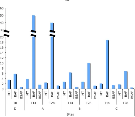
BSAFs were lower for organic contaminants on sediments A, B and C than in D. In general,
they were lower also for metals, except Cd, and PAHs for sediment A, Cd and PCBs for
sediment B, and As, Cd, Ni and Zn for sediment C. Both factors for Cd and BSAF for PAHs
**
**
29 were highly correlated to MT induction (ρ = 0.943, p < 0.01 and ρ = 0.886, p < 0.05
respectively) (Fig. 11 and 12), revealing a positive interaction between the contaminants.
Fig. 11 – MT (mg.g-1 whole soft tissue dry weight) and BAFs and BSAFs for Cd after 14 and 28 days of exposure to all sediments.
3.5
Histopathology
The Fig. 13 shows the digestive gland in cockles from sediment D in T0. The digestive gland
apparently seems normal, without alterations. In comparison with the sediment D, the
digestive gland of cockles from other sediments showed significant differences. Degradation
in the digestive gland tubule integrity is shown in the organisms from all sediments, except
the sediment D. The histological damages are present in most organisms and varied
depending on sediment and time of exposure. In general, there is a decrease of connective
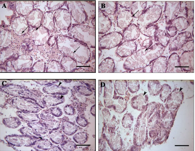
tissue (Fig. 14C, D, Fig. 15A-D, Fig. 16A-D). The excretory cells increased slightly in
sediment A (Fig. 14A, B) and highly in sediment C (Fig. 16A). The cells of tubules detached
from epithelium are identified in the cockles from sediment B, that is the most contaminated
(Fig. 15A-D) and at day 28 from sediment A (Fig. 14C, D) and C (Fig. 16C, D), where the
level of contaminants are lower. Increase of lumen size of the tubules of digestive gland is
observed in cockles from sediment C (Fig. 16B). Occasionally, hyperplasia of epithelial cells
was found in sediment B (Fig. 14A).
Fig. 13 - Histological sections stained with haematoxylin and eosin of digestive gland of C. edule. Scale bar: 50 µm.
31
Fig. 14 - Histological sections stained with haematoxylin and eosin of digestive gland of C. edule.
Fig. 15 - Histological sections stained with haematoxylin and eosin of digestive gland of C. edule.
33
Fig. 16 - Histological sections stained with haematoxylin and eosin of digestive gland of C. edule.
4
Discussion
In our study, BAF values generally presented a similar evolution, decreasing when sediment
TOM increased. A similar results was observed in a study of bioaccumulation of atrazine and
chlorpyrifos in the land worm Lumbriculus variegatus (Jantunen et al. 2008). An exception,
however, was observed regarding the organic contaminants. BAF of PCBs in the sediment C
is much lower than in other sediments, this may be due to the existence of a higher
concentration of PCBs in the sediment and cockles maintain the same capacity for
assimilation of PCBs, regardless of the initial concentration in the sediment. On the other
hand, the opposite was observed with PAHs and DDTs. The concentration of PAHs in the
sediment A was lower than in the other sediments and therefore, BAF of PAHs was much
higher. BAF of DDTs in sediment D was observed to be higher although the concentration of
DDTs in this sediment was very low. BAFs were more elevated in Cd and Ni (>> 1) and
DDTs (almost always > 1). For metals, BSAF value was always lower in sediment A (except
for Cd) and for organics it was always lower in sediment C. Theoretically, if the
bioavailability of contaminants depends only on the existence of a perfect correlation between
contaminant concentration and TOM, BSAF should be constant, but for the other sediments,
the BSAF values obtained were very variable. The large variability found in BSAF values
may be explained by the different quality of organic matter contents, sorption behavior and
other physico-chemical parameters affecting to the bioavailability of contaminants. Variable
values of BSAF have also been found in the bioaccumulation to Lumbriculus variegatus
(Jantunen et al. 2008) and on the bioaccumulation of cadmium and BDE-99 by Baltic Sea
benthic invertebrates (Thorsson et al. 2008). Significant positive correlations were found
between BAF and BSAF of Cd and MT. This indicates that cockles respond not only to the
concentration of Cd bioaccumulated but also to the relationship between the concentration of
Cd in the organism and in the sediment, i.e. the concentration at which they are exposed. This
35 (Costa et al. 2009). Significant positive correlations were found between BSAF of PAHs and
MT, being this response probably related with oxidative stress in cockles.
The time-of-exposure factor is known crucial for the bioaccumulation of contaminants (see
Luoma and Rainbow 2005). Cockles may need an adaptation period to reach the limit of
accumulation in relation to the concentration in the sediment. This is reflected in the total
values of BAFs for all sediments. The sediment A is the least polluted (SQG-Q = 0.082) and
has a total BAFs higher, and the sediment B is the most contaminated (SQG-Q = 0.313) and
has a total BAFs lower than the others. The sediment D is the second more contaminated
(SQG-Q = 0.181) but has BAF slightly below to sediment A. The cockles came from
sediment D, where they were exposed to local contamination throughout their lifes and it is
possible that a steady state could be attained between the levels of contaminants in the
districts compartments of the ecosystem.
Translocation from one site to another caused significant damages to the cockles’ digestive
gland. The histological analysis identified different responses of the organisms from different
stations. In a study of histopathological effects of petroleum hydrocarbons and heavy metals
on the American oyster, they related the histopathological lesions to certain contaminants but
also to salinity (Gold-Bouchot et al. 1995), this can be verified in our study because the
histopathological damages were found in the cockles from all sediments where they were
translocated, as the sediment A and C have less contamination that the sediment D according
to the SQG-Q calculated. Early lesions (day 14) and higher intensity are presented in the
cockles from sediment B and C; these sediment have higher contamination that the sediment
A, where the lesions are present only at day 28. This could indicate a greater effect caused by
contaminants than by other factors. The sediment A has a SQG-Q below 0.1, so that
contamination should not cause impact (MacDonald et al. 2004). However in several studies it
due to this, the cell-type composition of the digestive gland epithelium may result severely
altered (Zaldibar et al. 2008).
The slight increase in the number of excretory cells in cockles from sediment A at day 14
(Fig. 14A, B) could be due to the low level of contaminants (SQG-Q < 0.1) but at day 28 the
excretory cells are rarely identified due to the presence of severe lesions. Decrease of
connective tissue and dissagregation and unidentified cells were presented (Fig. 14C, D).
These damages do not appear to be caused by the contaminants, since they are in relatively
small quantities, unless non analysed chemicals were present in this sediment or due to the
local low TOM and FF, the bioavailability was higher. The highly increased of the number of
excretory cells in cockles from sediment C at day 14 (Fig. 16A, B) seems to be caused by
contaminants. This sediment has SQG-Q > 0.1, and according to MacDonald et al.(2004) this
could have a moderate impact in organisms. At day 28, the damages presented were loss of
epithelial tissue structure and epithelial lifting from tubule basal laminae (Fig. 16C, D), there
is an evident degradation in the digestive gland tubule integrity, so the excretory cells are
hardly identified. In cockles from sediment B, histological damages were very pronounced at
day 14 and 28. There is an early degradation in the digestive gland integrity, cells of tubules
detached from epithelium and slight decrease of connective tissue (Fig. 15A-D) and
occasionally hyperplasia of epithelial cells (Fig. 15A). This could be due to the sediment
which has SQG-Q higher than the other sediments but below 1, so that contaminants would
have a moderate impact.
Induction of MT is usually related with the metal concentrations. However, metals are not the
only factor in the MT induction, also other factors can interfere. In a study with Corbicula
fluminea, MT transcripts were higher in the digestive gland and the gills of bivalves collected
in July, where the result could be linked to the increasing metabolic activity related to the
37 is suggested that parasite infection in cockles can modulate MT synthesis that could
consequently interfere with the response of these protective proteins in case of metal
contamination. They monitored MT concentrations in cockles and they demonstrated that MT
levels were higher in parasitized individuals (Baudrimont et al. 2006). Cockles were dying
after a few months in systems of acclimatization, probably due to the development of
parasites found in these animals (Fig. 17). Therefore, MT induction is related to
environmental stressors. In our study, there was a decrease of MT levels in cockles from all
sediments and, the most significant decrease was been observed in organisms exposed to
sediment C. However, significant positive correlations between BSAF and MT were found for
PHAs, and between both BSAF and BAF and MT for Cd, which is in general accordance with
the known high inducibility of MT by this metal. For instance, in a study of Cd and Zn
bioaccumulation, C. fluminea revealed variations in MT concentrations strongly correlated to
progressive Cd and Zn bioaccumulation (Marie et al. 2006). On the other hand, the positive
correlation between Cd BSAFs and BAFs to MT suggests MT induction is dependent of the
availability of strong MT inducers, which adds up to yet another factor contributing to the
variability in MT responses as suggested by other surveys (Costa et al. 2008). The reduction
in MT contents, conversely, may be, at least partially, explained by the complex effects of
contaminant interactions. PAHs, for instance, found in the tested sediments, have been found
to suppress MT synthesis in prevence of strong metal inducers (Risso–De Faverney et al.,
Fig. 17 – Diversity of organisms found within C. edule in systems of acclimatization after a
few months. Many of these organisms were probably parasites.
Note that the images are not scale drawings and this figure just shows the variety of parasites found in the cockles.
This study revealed notable responses in cockles to different levels of contamination, hence, it
is suggested that C. edule responds to sediment–bound contamination, since this cockle
bioaccumulated and regulated (eliminated) both types of contaminants (Fig. 8, 9 and 10). For
some contaminants the concentration decreased, and this can be due to degradation of the
tissue or elimination for this way. Therefore, this cockle might be suitable for biomonitoring,
39 indicators of exposure need yet much research. In addition, the exposure of C. edule to other
types of sediments, particularly from more contaminated sites, can be used for the validation
of this bivalve as test species. This work shows the potential of the use of translocated cockle
References
Amiard J-C, Amiard-Triquet C, Barka S, Pellerin J, Rainbow PS (2006) Metallothioneins in
aquatic invertebrates: Their role in metal detoxification and their use as biomarkers. Aquatic
Toxicology 76:160–202
Baudrimont M, de Montaudouin X, Palvadeau A (2006) Impact of digenean parasite infection
on metallothionein synthesis by the cockle (Cerastoderma edule): A multivariate field
monitoring. Marine Pollution Bulletin 52:494–502
Biomarkers Definitions Working Group (2001) Biomarkers and surrogate endpoints:
preferred definitions and conceptual framework. Clin. Pharmacol. Therap. 69, 89–95
Bergayou H, Mouneyrac C, Pellerin J, Moukrim A (2009) Oxidative stress responses in
bivalves (Scrobicularia plana, Cerastoderma edule) from the Oued Souss estuary (Morocco).
Ecotoxicology and Environmental Safety 72:765–769
Bigot A, Doyen P, Vasseur P, Rodius F (2009) Metallothionein coding sequence
identification and seasonal mRNA expression of detoxification genes in the bivalve Corbicula
fluminea. Ecotoxicology and Environmental Safety 72:382– 387
Caeiro S, Costa MH, Ramos TB, Fernandes F, Silveira N, Coimbra A, Medeiros G, Painho M
(2005) Assessing heavy metal contamination in Sado Estuary sediment: An index analysis
approach. Ecological Indicators 5:151–169
Caetano M, Fonseca N, Cesário R, Vale C (2007) Mobility of Pb in salt marshes recorded by
41 Cajaraville MP, Bebianno MJ, Blasco J, Porte C, Sarasquete C, Viarengo A (2000) The use of
biomarkers to assess the impact of pollution in coastal environments of the Iberian Peninsula:
a practical approach. The Science of the Total Environment 247:295-311
Catarino J, Peneda MC, Santana F (1987) Estudo do Impacte da Indústria no Estuário do Rio
Sado. Estimativas da Poluição Afluente. DEII, INETI - Instituto Nacional de Engenharia e
Tecnologia Industrial, Lisbon, Portugal
Clesceri LS, Greenberg AE, Eaton AD (1999) Standard methods for examination of water &
wastewater, 20th edn. American Public Health Association, Baltimore
Cortesão C and Vale C (1995) Metals in Sediments of the Sado Estuary, Portugal. Marine
Pollution Bulletin Vol. 30, No. I, pp. 34-37
Costa PM, Repolho T, Caeiro S, Diniz ME, Moura I, Costa MH (2008) Modelling
metallothionein induction in the liver of Sparus aurata exposed to metal-contaminated
estuarine sediments. Ecotox Environ Saf 71:117-124
Costa PM, Santos HM, Peres I, Costa MH, Alves S, Capelo-Martinez JL, Diniz MS (2009)
Toxicokinetics of Waterborne Trivalent Arsenic in the Freshwater Bivalve Corbicula
fluminea. Arch Environ Contam Toxicol 57:338–347
Del Valls TA, Forja JM, Gómez-Parra A (1998) The use of multivariate analysis to link
sediment contamination and toxicity data to establish sediment quality guidelines: an example
in the Gulf of Cádiz (Spain). Ciencias Marinas 24:127-154
De Kock WC and Kramer KJM (1994) Active biomonitoring (ABM) by translocation of
bivalve molluscs. In: Kramer KJM (ed) Biomonitoring of coastal waters and estuaries. CRC
Ferreira AM, Martins M, Vale C (2003) Influence of diffuse sources on levels and distribution
of polychlorinated biphenyls in the Guadiana River estuary, Portugal. Mar Chem 89:175-184
Geret F, Serafim A, Bebianno MJ (2003) Antioxidant Enzyme Activities, Metallothioneins
and Lipid Peroxidation as Biomarkers in Ruditapes decussatus. Ecotoxicology 12:417-426
Gold-Bouchot G, Simá-Alvarez R, Zapata-Pérez O, Guemez-Ricalde J (1995)
Histopathological Effects of Petroleum Hydrocarbons and Heavy Metals on the American
Oyster (Crassostrea virginica) from Tabasco, México. Marine Pollution Bulletin Vol. 31,
Nos 4~12, pp. 439~445
Hédouin L, Pringault O, Metian M, Bustamante P, Warnau M (2007) Nickel bioaccumulation
in bivalves from the New Caledonia lagoon: Seawater and food exposure. Chemosphere
66:1449–1457
Huggett RJ, Kimerle RA, Mehrle PM, Bergman HL (eds) (1992) Biomarkers. Biochemical,
physiological, and histological markers of anthropogenic stress. Lewis Publishers, U.S.A.
Jantunen APK, Tuikka A, Akkanen J, Kukkonen JVK (2008) Bioaccumulation of atrazine and
chlorpyrifos to Lumbriculus variegatus from lake sediments. Ecotoxicology and
Environmental Safety 71:860–868
Jung K, Stelzenmüller V, Zauke G-P (2006) Spatial distribution of heavy metal
concentrations and biomass indices in Cerastoderma edule Linnaeus (1758) from the German
Wadden Sea: An integrated biomonitoring approach. Journal of Experimental Marine Biology
and Ecology 338:81–95
Koeman JH, Kohler-Gunther A, Kurelec B, Riviere JL, Versteeg D, Walker CH (1993)
43 Editors (1993) Biomarkers: Research and Application in the Assessment of Environmental
Health NATO ASI Series vol. H. 68, Springer, Berlin, pp. 1–13
Lee H (1992) Models, muddles, and mud: predicting bioaccumulation of sediment associated
pollutants. In: Burton, A.G. (Ed.), Sediment Toxicity Assessment. CRC, Boca Raton, FL, pp.
267–293
Livingstone DR (2001) Contaminant-stimulated reactive oxygen species production and
oxidative damage in aquatic organisms. Marine Pollution Bulletin Vol.42 No. 8, pp. 656-666
Long ER and MacDonald DD (1998) Recommended uses of empirically derived, sediment
quality guidelines for marine and estuarine ecosystems. Hum. Ecol. Risk Assess.
4:1019-1039.
Luoma S and Rainbow P (2005) Why is metal bioaccumulation so variable? Biodynamics as a
unifying concept. Environtal Science and Technology. 39:1921–1931.
Machreki-Ajmi M, Ketata I, Ladhar-Chaabouni R, Hamza-Chaffai A (2008) The effect of in
situ cadmium contamination on some biomarkers in cerastoderma glaucum. Ecotoxicology
17:1–11
MacDonald DD, Carr S, Calder F, Long E, Ingersoll C (1996) Development and evaluation of
sediment quality guidelines for Florida coastal waters. Ecotoxicology 5:253-278
MacDonald DD, Carr RS, Eckenrod D, Greening H, Grabe S, Ingersoll CG, Janicki S, Janicki
T, Lindskoog RA, Long ER, Pribble R, Sloane G, Smorong DE (2004) Development,
evaluation, and application of sediment quality targets for assessing and managing
Marie V, Baudrimont M, Boudou A (2006) Cadmium and zinc bioaccumulation and
metallothionein response in two freshwater bivalves (Corbicula fluminea and Dreissena
polymorpha) transplanted along a polymetallic gradient. Chemosphere 65:609–617
Martins M, Ferreira AM, Vale C (2008) The influence of Sarcocornia fruticosa on retention of
PAHs in salt marshes sediments (Sado estuary, Portugal). Chemosphere 71:1599-1606
Martoja R and Martoja M (1967) Initiation aux Tecniques de l’Histologie Animal. Masson &
Cie, Paris, 345 pp.
Peakall DB and Shugart LR (eds) (1993) Biomarkers. Research and application in the
assessment of environmental health. Springer-Verlag. Berlin, Heidelberg.
Risso-de Faverney C, Lafaurie M, Girard J-P, Rahmani R (2000). Effects of heavy metals and
3-methylcholanthrene on expression and induction of CYP1A1 and metallothionein levels in
trout (Oncorhynchus mykiss) hepatocyte cultures. Environmental and Toxicological
Chemistry. 19:2239–2248
Serafim A and Bebianno MJ (2009) Metallothionein role in the kinetic model of copper
accumulation and elimination in the clam Ruditapes decussates. Environmental Research
109:390–399
Solé M, Kopecka-Pilarczyk J, Blasco J (2009) Pollution biomarkers in two estuarine
invertebrates, Nereis diversicolor and Scrobicularia plana, from a Marsh ecosystem in SW
Spain. Environment International 35:523–531
Syasina IG, Vaschenko MA, Zhadan PM (1997). Morphological Alterations in the Digestive
Diverticula of Mizuhopecten yessoensis (Bivalvia: Pectinidae) from Polluted Areas of Peter
45 Thorsson MH, Hedman JE, Bradshaw C, Gunnarsson JS, Gilek M (2008) Effects of settling
organic matter on the bioaccumulation of cadmium and BDE-99 by Baltic Sea benthic
invertebrates. Marine Environmental Research 65:264–281
United States Environmental Protection Agency (USEPA) (1995) CRITFC exposure study.
Water Quality Criteria and Standards Newsletter. USEPA, Washington, DC
Zaldibar B, Cancio I, Soto M, Marigómez I (2007) Digestive cell turnover in digestive gland
epithelium of slugs experimentally exposed to a mixture of cadmium and kerosene.
Chemosphere 70:144–154
Zaldibar B, Cancio I, Soto M, Marigómez I (2008) Changes in cell-type composition in
digestive gland of slugs and its influence in biomarkers following transplantation between a
relatively unpolluted and a chronically metal-polluted site. Environmental Pollution 156:367–
47 Annex I - Metal and organic concentrations of sediments from sites D, A, B and C.
Sites
D A B C
TELa PELb
PEL-Qc
PEL-Q
PEL-Q
PEL-Q Metallic (mg.kg-1 sediment dry
weight) ±γ
As 7.24 41.6 20,55 ± 0,41* 0.49 7.25 ± 0.15* 0.17 27.43 ± 0.55* 0.66 12.38 ± 0.25* 0.30
Cd 0.68 4.21 0,23 ± 0,00 0.05 0.04 ± 0.00 0.01 0.22 ± 0.00 0.05 0.15 ± 0.00 0.04
Cu 18.7 108 63,67 ± 1,27* 0.59 22.57 ± 0.45* 0.21 167.32 ± 3.35** 1.55 41.18 ± 0.82* 0.38
Ni 15.9 42.8 26,12 ± 0,52* 0.61 12.97 ± 0.26 0.30 33.67 ± 0.67* 0.79 9.03 ± 0.18 0.21
Pb 30.2 112 30,92 ± 0,62* 0.28 23.70 ± 0.47 0.21 66.49 ± 1.33* 0.59 45.17 ± 0.90* 0.40
Zn 124 271 232,99 ± 4,66* 0.86 147.48 ± 2.95* 0.54 312.23 ± 6.24** 1.15 87.75 ± 1.76 0.32
Organic (µg.kg-1 sediment dry weight) ±γ
PAHs 3 – ring
Acenaphthene 6.71 88.9 2,09 ± 0,36 0.02 1.41 ± 0.24 0.02 9.42 ± 1.60* 0.11 4.19 ± 0.71 0.05
Acenaphthylene 5.87 128 4,64 ± 0,79 0.04 0.24 ± 0.04 0.00 1.83 ± 0.31 0.01 1.95 ± 0.33 0.02
Anthracene 46.9 245 5,72 ± 0,97 0.02 1.03 ± 0.17 0.00 10.60 ± 1. 0.04 15.34 ± 2.61 0.06
Fluorene 21.2 144 3,56 ± 0,61 0.02 1.32 ± 0.22 0.01 8.70 ± 1.48 0.06 8.03 ± 1.37 0.06
Phenanthrene 86.7 544 18,67 ± 3,17 0.03 7.96 ± 1.35 0.01 50.77 ± 8.63 0.09 54.09 ± 9.20 0.10
4 – ring
Benz(a)anthracene 74.8 693 1,04 ± 0,18 0.00 4.53 ± 0.77 0.01 64.60 ± 10.98 0.09 86.52 ± 14.71* 0.12
Chrysene 108 846 3,49 ± 0,59 0.00 2.20 ± 0.37 0.00 28.31 ± 4.81 0.03 37.19 ± 6.32 0.04
Fluoranthene 113 1494 185,54 ± 31,54* 0.12 18.05 ± 3.07 0.01 170.80 ± 29.04* 0.11 184.30 ± 31.30* 0.12
Pyrene 153 1398 171,67 ± 29,18* 0.12 14.66 ± 2.49 0.01 131.74 ± 22.40 0.09 171.39 ± 29.14* 0.12
5 – ring
Benzo(a)pyrene 88.8 793 74,94 ± 12,74 0.09 7.56 ± 1.28 0.01 69.81 ± 11.87 0.09 85.88 ± 14.60 0.11
Benzo(b)fluoranthene 56.53 9.61 6.77 ± 1.15 60.86 ± 10.35 70.25 ± 11.94
Benzo(e)pyrene 46.64 7.93 5.12 ± 0.87 56.73 ± 9.64 62.76 ± 10.67
Benzo(k)fluoranthene 25.04 4.26 4.16 ± 0.71 32.21 ± 5.48 40.18 ± 6.83
Dibenzo(a,h)anthracene 6.22 135 7,06 ± 1,20* 0.05 0.74 ± 0.13 0.01 7.45 ± 1.27* 0.06 6.99 ± 1.19* 0.05
Perylene 40.06 ± 6.81 4.69 ± 0.80 86.97 ± 14.78 209.16 ± 35.56
6 – ring