ISSN 0001-3765 www.scielo.br/aabc
Time evolution of the South Atlantic Magnetic Anomaly
GELVAM A. HARTMANN and IGOR G. PACCA
Departamento de Geofísica, Instituto de Astronomia, Geofísica e Ciências Atmosféricas Universidade de São Paulo, Rua do Matão, 1226, Cidade Universitária
05508-090 São Paulo, SP, Brasil
Manuscript received on October 22, 2007; accepted for publication on March 26, 2009; contributed byIGORG. PACCA*
ABSTRACT
The South Atlantic Magnetic Anomaly (SAMA) is one of the most outstanding anomalies of the geomagnetic field. The SAMA secular variation was obtained and compared to the evolution of other anomalies using spherical harmonic field models for the 1590–2005 period. An analysis of data from four South American observatories shows how this large scale anomaly affected their measurements. Since SAMA is a low total field anomaly, the field was separated into its non-dipolar, quadrupolar and octupolar parts. The time evolution of the non-dipole/total, quadrupolar/total and octupolar/total field ratios yielded increasingly high values for the South Atlantic since 1750. The SAMA evolution is compared to the evolution of other large scale surface geomagnetic features like the North and the South Pole and the Siberia High, and this comparison shows the intensity equilibrium between these anomalies in both hemispheres. The analysis of non-dipole fields in historical period suggests that SAMA is governed by (i) quadrupolar field for drift, and (ii) quadrupolar and octupolar fields for intensity and area of influence. Furthermore, our study reinforces the possibility that SAMA may be related to reverse fluxes in the outer core under the South Atlantic region.
Key words:geomagnetic field, non-dipole field anomalies, secular variation, South Atlantic Magnetic Anomaly.
INTRODUCTION
The morphology and time variation of the geomagnetic field result from magnetohydrodynamic processes that take place in the Earth’s outer core. The study of the main characteristics of the field observed at the Earth’s surface, together with their variations in historical and geological time scales, has enabled the elaboration of numerical geodynamo simulations that have been suc-cessful in providing explanations for features of the field such as its predominantly dipolar character, secular vari-ation and field reversals (e.g. Glatzmaier and Roberts 1995a, b, Kageyama et al. 1995, Kageyama and Sato 1997, Kuang and Bloxham 1999). The results of geo-dynamo models are compared with the inversion of the
*Member Academia Brasileira de Ciências Correspondence to: Gelvam A. Hartmann E-mail: [email protected]; [email protected]
geomagnetic field data at the core-mantle boundary (CMB) (e.g. Roberts and Glatzmaier 2000).
entrance of high energy particles in the magnetosphere (Heynderickx 1996, Heirtzler 2002). This increase of cosmic ray particles may affect objects that orbit Earth such as satellites and space stations (e.g. Badhwar 1997, Buhler et al. 2002, Badhwar et al. 2002, Barde et al. 2002, Willis et al. 2004). These effects may be detected also on the surface of Earth as disturbances in commu-nications and induced currents in pipelines and trans-mission lines (Padilha 1995, Pinto et al. 2004, Trivedi et al. 2005). These SAMA effects have also been the object of space geophysics research (Pinto Jr and Gon-zalez 1986, 1989, Pinto Jr et al. 1989, 1990, 1992, 1997, Fiandrini et al. 2004), in the study of trapped electrons in radiation belts.
Some authors have related SAMA to the North-ern-Southern hemisphere asymmetry of the geomag-netic field (Fraser-Smith 1987, Pinto Jr et al. 1992, Heynderickx 1996, Heirtzler 2002). The eccentric di-pole that best represents the geomagnetic field is dis-placed from the Earth’s center towards Northwestern Pacific (21.47◦N; 144.77◦E) (Fraser-Smith 1987). The
antipodal point would then be in the Southern Atlantic, but rather far from the SAMA center. However, the SAMA behavior may indicate that these asymmetries may be connected to the general decrease of the dipo-lar field and to the significant increase of the non-dipodipo-lar field in the Southern Atlantic (e.g. Bloxham et al. 1989, Bloxham and Jackson 1992, Hulot et al. 2002, Olson 2002, Pacca and Hartmann 2005, G.A. Hartmann, un-published data1). Another remarkable feature of the ge-omagnetic field is the Siberia High, a region where field intensities are considerably higher than those for com-parable latitudes. This anomaly, SAMA and the geo-magnetic poles are the most important features of the geomagnetic field, and their investigation and compari-son to each other can provide important information on the dynamics of the geomagnetic field.
Using spherical harmonics field models, such as those obtained by Jackson et al. (2000) for the his-torical period (1590–1990) (called GUFM1) and the IGRF (International Geomagnetic Reference Field) and DGRF (Definitive Geomagnetic Reference Field) mod-els for the past century, the main characteristics of the field secular variation are compared to SAMA. We also
1Online version: http://www.teses.usp.br/
show how the SAMA variation affected measurements of four South American observatories, the non-dipolar source character of the South Atlantic magnetic field, and the relation between SAMA and other geomagnetic anomalies. This analysis of the geomagnetic field may be able to lead to helpful links for discussing field gen-eration processes in the CMB. The essential contents of this article were part of a MSc. Dissertation presented at the University of São Paulo (G.A. Hartmann, unpub-lished data1).
LOCATION DETERMINATION FOR SAMA AND OTHER ANOMALIES
The time and space variation of SAMA depends on the morphological behavior of the whole field. The SAMA center has been taken as the locus of minimum inten-sity in the South Atlantic, as proposed by Heynderickx (1996). A similar procedure was used to define the center of other anomalies like the North Pole (NP), the South Pole (SP) and the Siberia High (SH) as the max-imum global intensities in a region. The center of non-dipole anomalies has also been taken as points of max-imum/minimum intensity. These anomaly centers are computed from spherical harmonic expansions of the geomagnetic potential, i.e. geomagnetic field models. The field models used in this study are DGRF, IGRF and GUFM1. DGRF and IGRF models provide sets of Gauss coefficients up to spherical harmonic degree n = m = 10 (or 13, for IGRF 2000 onwards) and
GUFM1 up ton=m=14. ComponentsX,Y andZof the geomagnetic field can be expressed as functions of time(t)and spherical coordinates(r, θ, λ)by:
X(r, θ, λ,t)=
∞ X n=1 m X m=0
gnm(t)cosmλ
+hmn(t)sinmλd P m n (θ ) dθ
a r
n+2 (1)
Y(r, θ, λ,t)= 1 sinθ ∞ X n=1 m X m=0
mgnm(t)sinmλ
+mhmn(t)cosmλPnm(θ ) a
r n+2
(2)
Z(r, θ, λ,t)=
∞ X n=1 m X m=0
gnm(t)cosmλ
+hmn(t)sinmλ Pnm(θ )a r
-90 -60 -30 0 30 60 90
-90 -60 -30 0 30 60 90
-180 -120 -60 0 60 120 180
-90 -60 -30 0 30 60 90
-180 -120 -60 0 60 120 180
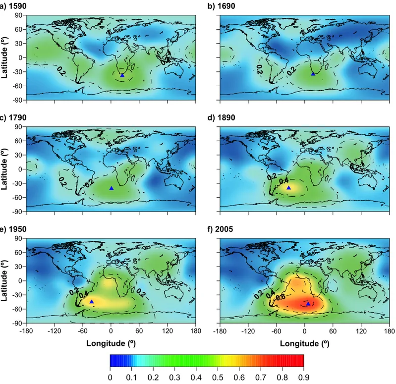
22000 30000 38000 46000 54000 62000 70000 78000
Fig. 1 – Examples of geomagnetic field total intensity maps obtained with GUFM1 and IGRF models. The red triangle indicates the SAMA center, and the 28000nT contours shows the SAMA range influence area.
wherea is Earth’s mean radius (6371.2 km). Pnm(θ )is
associate Legendre polynomials and gnm(t) and hmn(t)
are field models Gauss coefficients (e.g. Langel 1987). And the total field will be:
B=
X2+Y2+Z21/2 (4)
The resolution of maximum/minimum intensity points location will depend on the resolution of the spherical harmonic models that are used. The contributions of non-dipolar(n >1), quadrupolar(n=2)and octupolar
(n=3)fields have also been calculated in an attempt to
characterize the SAMA signatures (Section non-dipolar field and Fig. 6).
SAMA: THE MAIN FEATURES AND TIME-EVOLUTION
THEANOMALYCENTER AND ITSPATH
GUFM1 models prior to 1840 involve an approxima-tion to determine the magnitude of B. These models assume that g10 was decreasing at a rate of 15nT/year prior to 1840. This assumption was necessary because direct absolute intensity measurements were not avail-able for the time before 1840 (e.g. Barraclough 1974, Jackson et al. 2000). Nevertheless, it is possible to an-alyze the main characteristics of the geomagnetic field morphology. Some examples of total intensity plots ob-tained with field models are shown in Figure 1. Time and space variations of SAMA follow in part the mor-phological behavior of the field in general.
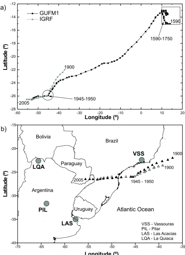
Figure 2a shows the drift of the SAMA center for the past 415 years in five year intervals. For this period, SAMA shows a westward drift of 70◦ (≈ 0.17◦/year)
and a southward drift of 12◦(≈0.03◦/year). The whole
interval may be divided into three sectors:
(i) 1590–1750, when SAMA presented variations of
≈ 6◦in longitude and≈1.5◦in latitude;
(ii) 1750 to 1945–1950, when both westward and southward drifts were approximately constant, and
(iii) 1945–2005, when latitude variation was much smaller and practically there was only a westward drift.
Therefore SAMA shows a general westward drift, but with different rates for certain intervals such as those before and after 1750.
For the past 105 years GUFM1 can be compared to IGRF models. Figure 2b shows a second diagram of the SAMA space variation where four South Ameri-can observatories that are located near to its center are indicated. For the past century the SAMA southern dis-placement can be separated into two intervals. After 1945–1950, the latitude variation was much smaller than that for the previous period between 1900–1945. The mean variation rate for the past 60 years was very small, practically without a change in latitude. The west-ward drift rates obtained with particle fluxes (Badhwar 1997, 2002, Buhler et al. 2002) are approximately 0.1◦/
year higher than the ones obtained with the minimum field for the past 105 years. The particle flux data in-dicate a northern displacement while the minimum field indicates a southern displacement.
INTENSITY
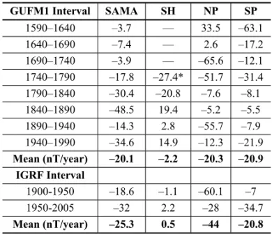
The SAMA center intensity changes with variable rates for different time intervals. Figure 3 shows the SAMA intensity variation for the past 415 years. During this interval, the SAMA intensity decreased about 8500nT, with an average decrease of 22.7nT/year. Intensity vari-ations (intensity first derivatives) are presented in Fig-ure 3 and in Table I. Between 1590–1750, intensity variations were rather low when compared to higher val-ues after this interval. Figure 3 shows variations up to –65nT/year between 1850–1900, that seem to be mean-ingful for a low latitude anomaly.
TABLE I
Intensity variation (nT/year) at the SAMA, SH, NP and
SP center for the past 415 years.
GUFM1 Interval SAMA SH NP SP
1590–1640 –3.7 — 33.5 –63.1
1640–1690 –7.4 — 2.6 –17.2
1690–1740 –3.9 — –65.6 –12.1
1740–1790 –17.8 –27.4* –51.7 –31.4 1790–1840 –30.4 –20.8 –7.6 –8.1 1840–1890 –48.5 19.4 –5.2 –5.5 1890–1940 –14.3 2.8 –55.7 –7.9 1940–1990 –34.6 14.9 –12.3 –21.9 Mean (nT/year) –20.1 –2.2 –20.3 –20.9
IGRF Interval
1900-1950 –18.6 –1.1 –60.1 –7
1950-2005 –32 2.2 –28 –34.7
Mean (nT/year) –25.3 0.5 –44 –20.8
*Variation for period between 1770 to 1790.
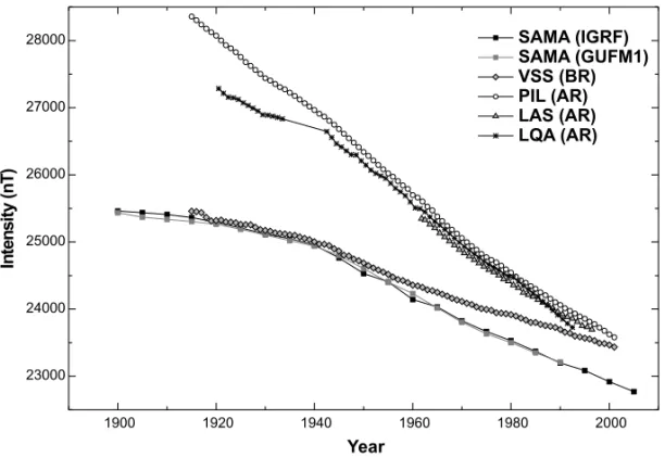
The SAMA effect is visible in some geomag-netic observatories intensity data. The Vassouras (VSS: 22◦24′S, 43◦39′W) observatory in Brazil and Pilar
(PIL: 31◦39′S, 63◦52′W), Las Acacias (LAS: 35◦S,
57◦42′W) and La Quiaca (LQA: 22◦36′S, 65◦36′W) in
b)
-70 -65 -60 -55 -50 -45 -40 -35 -40
-35 -30 -25 -20 -15
1900
2005
Atlantic Ocean
Brazil
Uruguay Argentina
Paraguay Bolivia
1945 - 1950
VSS - Vassouras PIL - Pilar LAS - Las Acacias LQA - La Quiaca
1900 -60 -50 -40 -30 -20 -10 0 10 20 -28
-26 -24 -22 -20 -18 -16 -14 -12
1590-1750
1945-1950 1900
2005
1590 GUFM1
IGRF
a)
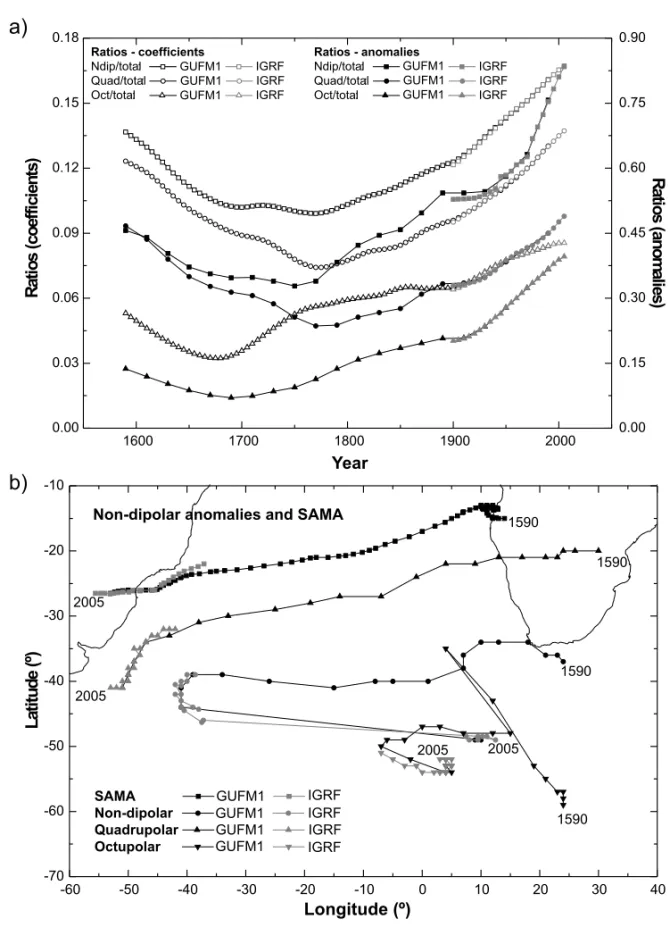
Fig. 2 – (a) the SAMA center trajectory from 1590 to 2005. Note that the 1590–1750 interval corresponds to lower drift rates; (b) the SAMA center trajectory from 1900 to 2005 in relation to the location of four South American Geomagnetic Observatories: Vassouras (VSS) in Brazil, and Las Acacias (LAS), La Quiaca (LQA) and Pilar (PIL), in Argentina.
high variation for 1945–1950, but there is not much vari-ation for PIL. This period is critical because it corre-sponds to the SAMA center change in trajectory.
Between 1915 and 1940, the SAMA center was ap-proaching VSS, reaching a minimum distance of less than 500 km. The center is presently in an approximately equidistant position from the four observatories. For this
32000 10
1600 1700 1800 1900 2000
22000 23000 24000 25000 26000 27000 28000 29000 30000 31000
GUFM1 IGRF
-70 -60 -50 -40 -30 -20 -10 0
GUFM1 IGRF
Fig. 3 – Total field intensity variation at the SAMA center for the past 415 years. The left ordinates correspond to total intensity and the right ordinates the first derivative of total intensity.
1900 1920 1940 1960 1980 2000
23000 24000 25000 26000 27000 28000
Fig. 4 – Total field intensity variations for the VSS, PIL, LAS, and LQA Observatories.
NON-DIPOLARFIELD
The non-dipole field has been increasing with time for the past century and since SAMA is a low total field anomaly, considering the four parts (total, non-dipolar,
in--90 -60 -30 0 30 60 90
-90 -60 -30 0 30 60 90
-180 -120 -60 0 60 120 180
-90 -60 -30 0 30 60 90
-180 -120 -60 0 60 120 180
0 0.1 0.2 0.3 0.4 0.5 0.6 0.7 0.8 0.9
Fig. 5 – The non-dipole/total (NPT) field ratio, showing the drift of the non-dipole field anomaly presently in the South Atlantic. Note the increase in intensity and influence area of the non-dipole field.
dicated by blue triangles and they have been obtained for twenty year intervals for the past 415 years. A simi-lar procedure was used for obtaining the quadrupole and octupole contributions.
Figure 6a shows time variation ratios for the summation of coefficients for non-dipolar/total (NPT), quadrupolar/total (QPT) and octupolar/total (OPT). The left side values correspond to the ratios of the models coefficients, while the right side values correspond to the maximum anomalies in the South Atlantic. The non-dipole part of the global field is presently about 17% of
the total field. However, in the past century, the non dipole part increased about 5%, whereas the dipole field decreased also 5%. After≈ 1750 the quadrupolar and
1600 1700 1800 1900 2000 0.00
0.03 0.06 0.09 0.12 0.15 0.18
Ndip/total: GUFM1 IGRF Quad/total: GUFM1 IGRF Oct/total: GUFM1 IGRF
0.00 0.15 0.30 0.45 0.60 0.75 0.90
Ndip/total: GUFM1 IGRF Quad/total: GUFM1 IGRF Oct/total: GUFM1 IGRF
a)
-60 -50 -40 -30 -20 -10 0 10 20 30 40
-70 -60 -50 -40 -30 -20 -10
2005 2005 2005
2005
1590 1590
1590 1590
GUFM1 IGRF GUFM1 IGRF GUFM1 IGRF GUFM1 IGRF
b)
Fig. 6 – Comparison of the non-dipolar contributions. In (a), left: the models coefficients ratios (NPT, QPT and OPT); right: the maximum (anomalies) non-dipole fields (NPT, QPT and OPT). In (b), drifts of the maximum non-dipole fields obtained in (a) and SAMA.
Figure 6b compares the drift of these maxima to the SAMA drift. The behavior of NPT and OPT is quite dif-ferent from that of QPT and SAMA because non-dipole sources do not follow the westward drift systematically.
remark-able correlation between the drift of the QPT maximum and that of the SAMA center. From 1750 to present, practically the whole South Atlantic shows high NPT, QPT and OPT ratios, as shown in Figure 6a. Therefore, the high degree terms that correspond to the non-dipole fields have been increasing significantly, indicating the importance of these terms for SAMA.
DISCUSSION
The main characteristics of the SAMA time and space evolution are a decrease in total geomagnetic field in-tensity, increase in the influence area and both westward and southward drifts. Secular variation shows that the SAMA morphology is influenced by non-dipole field components. A comparison with the evolution of other large scale anomalies may yield interesting results.
INFLUENCE OFNON-DIPOLEFIELD ON THESAMA EVOLUTION
Intensity variations depend strongly ong10. According to some authors, the dipolar core field observed on the surface of the Earth (main field) exceeds the non-dipole field in a time average of a few thousand years, when the axial dipole is predominant (eg. Carlut et al. 1999). According to Olson and Amit (2006), the present dipole decrease could be transient as core fluid motion may re-duce the dipole field by transferring energy to other mag-netic field harmonics through a turbulent process. This could be inferred from the magnetic flux distribution at the CMB caused by core fluid flow. Non-dipole terms would then fluctuate in a time scale of centuries.
For the historical period, high variation rates of non-dipole sources in the South Atlantic seem to have strong influence on the SAMA behavior, as suggested in the comparison between the drifts of SAMA and that of the quadrupole field anomaly (Fig. 6b). The total inten-sity of this anomaly during the whole historical period is only a few thousand nT lower than the SAMA inten-sity. Therefore, the influence of the dipolar field in the SAMA region of influence is small.
Since the non-dipolar time constants are smaller than that of the dipole, energy must be transferred to more than one non-dipole component (Olson and Amit 2006). This would explain the quadrupolar anomaly significant increase in South America as well as that of the octupolar
anomaly in Southern Africa and they must influence the SAMA area directly since the 28000nT contour on the total intensity map for 2005 extends from South America to Southern Africa as shown in Figure 1.
SAMAANDOTHERGEOMAGNETICFIELDANOMALIES
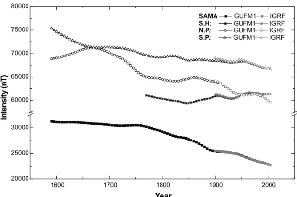
The geomagnetic field morphology is important for the SAMA evolution. Therefore, SAMA is compared to other large scale geomagnetic anomalies, like the SH, NP and SP. Figure 7 shows field intensity varia-tions at the focus of isolines corresponding to SAMA, SH, NP, and SP for the period between 1590–2005. At first, there seems to be no direct connection among these variations. The NP intensities are lower than those of the SP. However, both poles show a decrease in their in-tensities. Table I shows the variation rates for the four anomalies, and the data indicate a higher variation for NP. It can also be noted that the addition of SP and SAMA mean variations indicates values that are simi-lar to those corresponding to the summation of NP and SH mean variations. This may be interpreted as a conse-quence of the Alfven theorem (Bondi and Gold 1950, Jackson 2003) that states that the total magnetic flux across a spherical surface is invariable. Fluxes in both hemispheres must be conserved, which may mean that intensities in the southern hemisphere may result from the balance between SAMA and SP, while in the north-ern hemisphere the balance is between NP and SH.
SAMA also shows a decreasing intensity for the past 250 years, but the contribution of the non-dipole field has been important for its region of influence. From 1590 to 1750, the total field intensities were approxi-mately stable, while the non-dipole field was decreasing. From 1750 onwards, total intensities decrease while the non-dipole field increases.
1600 1700 1800 1900 2000 20000
25000 30000 60000 65000 70000 75000 80000
: GUFM1 IGRF : GUFM1 IGRF : GUFM1 IGRF : GUFM1 IGRF
Fig. 7 – Total field intensity at the focus for SAMA, SH, NP, and SP from 1590 to 2005. The SH becomes apparent in after 1770.
SAMA and other major features of the geomagnetic field, such as the poles (NP and SP), SH and non–dipole field anomalies, may be taken as “mobile observatories” since the use of the anomalies points of maximum or min-imum may indicate field variations that are not evident when only observatory data and models are used.
The 1590–1750 period shows low SAMA variation rates and drift but, after 1750, time and space variations increase, and this coincides with the increase of non-dipole sources and the appearance of SH around 1770. A correlation between the different phenomena is com-plex, but the phenomenology may be approached by us-ing geodynamo concepts. Accurate geomagnetic field maps at the CMB show persistent reverse flux regions in the South Atlantic (e.g. Bloxham and Gubbins 1985, Bloxham 1987, Gubbins 1987, Gubbins and Bloxham 1987, Bloxham and Jackson 1989, 1992, Bloxham et al. 1989, Jackson et al. 2000, Olson and Amit 2006). Therefore, the SAMA observed at Earth’s surface is re-lated to CMB field morphology; in other words, SAMA seems to be a consequence of these reverse fluxes.
CONCLUSIONS
SAMA is a long-lived total intensity anomaly. Besides the usual westward drift, it has also had a predominantly southward drift with variable rates for the past 415 years.
The total field intensity at the anomaly center shows vari-able rates of decrease during this period. The space and time evolution of SAMA has been obtained with GUFM1 and IGRF models. Archaeomagnetic data indicate decay rates for the dipole moment that are lower than those for the present time and Gubbins et al. (2006) propose that the present decrease rate began around 1840. However, in spite of GUFM1 models applying a –15nT/year lin-ear extrapolation forg01for the period before 1840 (e.g. Barraclough 1974, Jackson et al. 2000), the obtained SAMA main characteristics such as drift, intensity vari-ations, comparison with the non-dipolar field and with other anomalies seem to be quite coherent.
The analysis of the non-dipole geomagnetic field for the historical period shows that SAMA is an anom-aly that is governed by quadrupolar and octupolar terms. The SAMA center drift (westward and southward) seems to be characterized by quadrupolar field. Intensity vari-ation and area of influence is governed by quadrupolar and octupolar terms.
A comparison between the SAMA evolution and that of other major geomagnetic features may be help-ful in predicting the future field, as for example in the hypothesis that the present field might be in the course of a reversion process (eg. Gubbins 1987), because pres-ently the major geomagnetic features seem to equilibrate the total magnetic flux on Earth’s surface in both hemi-spheres. However, a better understanding of this and other phenomena will be possible only with the progress of geomagnetic dynamo and CMB flux models.
ACKNOWLEDGMENTS
The authors thank Conselho Nacional de Desenvolvi-mento Científico e Tecnológico (CNPq), Coordenação de Aperfeiçoamento de Pessoal de Nível Superior (CAPES) and Fundação de Apoio à Pesquisa do Estado de São Paulo (FAPESP) (grant 2005/57782-4) for financial sup-port to this work. They also thank two anonymous ref-erees for their very helpful comments.
RESUMO
A Anomalia Magnética do Atlântico Sul (SAMA) é uma das maiores anomalias do campo geomagnético. A variação secu-lar da SAMA foi obtida e comparada com a evolução de outras anomalias usando modelos de campo por harmônicos esféri-cos para o período de 1590–2005. Uma análise dos dados de quatro observatórios da América do Sul mostra como esta ano-malia de grande escala afetou suas medidas. Como a SAMA é uma anomalia de campo total baixo, o campo foi separado nas componentes não-dipolar, quadrupolar e octupolar. A evo-lução temporal das razões dos campos não-dipolar/total, qua-drupolar/total e octupolar/total mostram valores elevados para o Atlântico Sul desde 1750. A evolução da SAMA é com-parada com a evolução de outras grandes feições geomagnéti-cas de superfície como os pólos Norte e Sul e o Alto da Sibéria, e sua comparação mostra o equilíbrio de intensidade entre es-tas anomalias em ambos os hemisférios. A análise dos campos não-dipolares no período histórico sugere que a SAMA é regida
(i) pelo campo quadrupolar para a deriva, e (ii) pelos campos quadrupolar e octupolar para a intensidade e área de influência. Além disso, este estudo reforça a possibilidade de que a SAMA possa estar relacionada aos fluxos reversos no núcleo externo sob a região do Atlântico Sul.
Palavras-chave: campo geomagnético, anomalias do campo não-dipolar, variação secular, Anomalia Magnética do Atlân-tico Sul.
REFERENCES
BADHWARGD. 1997. Drift rate of the South Atlantic Anom-aly. J Geophys Res 102(A2): 2343–2349.
BADHWAR GD, ATWELL W, REITZ G, BEUJEANR AND
HEINRICHW. 2002. Radiation measurements on the Mir
Orbital Station. Radiat Meas 35: 393–422.
BARDE S, CUETO J, ECOFFET R, FALGUÈRE D, NUNS
T, DUZELLIER S, BOSCHER D, BOURDARIE S AND
TSOURILO I. 2002. Radiation Environment Measure-ments with SPICA On-Board the MIR Station. IEEE Trans Nuc Sci 49: 1333–1339.
BARRACLOUGHDR. 1974. Spherical Harmonic Analyses of the Geomagnetic Field for Eight Epochs between 1600 and 1910. Geophys J R Astron Soc 36: 497–513. BLOXHAMJ. 1987. Simultaneous Stochastic Inversion for
Geomagnetic Main Field and Secular Variation 1. A Large-Scale Inverse Problem. J Geophys Res 92: 11597– 11608.
BLOXHAMJANDGUBBINSD. 1985. The secular variation of Earth’s magnetic field. Nature 317: 777–781. BLOXHAMJANDJACKSONA. 1989. Simultaneous
Stochas-tic Inversion for GeomagneStochas-tic Main Field and Secular Variation 2. 1820–1980. J Geophys Res 94: 15753– 15769.
BLOXHAMJANDJACKSONA. 1992. Time-Dependent
Map-ping of the Magnetic Field at the Core-Mantle Boundary. J Geophys Res 97: 19537–19563.
BLOXHAMJ, GUBBINSDANDJACKSONA. 1989. Geomag-netic Secular Variation. Phil Trans R Soc London A 329: 415–502.
BONDIHANDGOLDT. 1950. On the generation of mag-netism by fluid motion. Mon Not R Astron Soc 110: 607– 611.
BÜHLER P, ZEHNDER A, KRUGLANSKIM, DALYE AND
ADAMSL. 2002. The high-energy proton fluxes in the
CARLUT J, COURTILLOT VAND HULOT G. 1999. Over how much time should the geomagnetic field be averaged to obtain the mean paleomagnetic field? Terra Nova 11: 239–243.
CHAPMANSANDBARTELSJ. 1940. Geomagnetism, vol 2. Oxford: University Press, 1049 p.
FIANDRINIEET AL. 2004. Protons with kinetic energy E> 70MeV trapped in the Earth’s radiation belts. J Geophys Res 109: A102014.
FRASER-SMITHAC. 1987. Centered and Eccentric
Geomag-netic Dipoles and their Poles, 1600–1985. Rev Geophys 25: 1–16.
GLATZMAIER GA ANDROBERTS P H. 1995a. A three-dimensional convective dynamo solution with rotating and finitely conducting inner core and mantle. Phys Earth Planet Int 91: 63–75.
GLATZMAIER GA ANDROBERTS P H. 1995b. A three-dimensional self-consistent computer simulation of a geo-magnetic field reversal. Nature 377: 203–209.
GUBBINS D. 1987. Mechanisms for geomagnetic polarity
reversals. Nature 326: 167–169.
GUBBINSD ANDBLOXHAM J. 1987. Morphology of the geomagnetic field and implications for the geodynamo. Nature 325: 509–511.
GUBBINSD, JONESA L ANDFINLAYCC. 2006. Fall in Earth’s Magnetic Field is Erratic. Science 312: 900–902. HEIRTZLER JR. 2002. The Future of the South Atlantic Anomaly and implications for radiation damage in space. J Atmos Solar-Terr Phys 64: 1701–1708.
HEYNDERICKXD. 1996. Comparison between methods to
compensate for the secular motion of the South Atlantic Anomaly. Radiat Meas 26: 369–373.
HULOTG, EYMINC, LANGAISB, MANDEAMANDOLSEN
N. 2002. Small-scale structure of the geodynamo inferred from Oersted and Magsat satellite data. Nature 416: 620– 623.
JACKSONA. 2003. Intense flux spots on the surface of the
Earth’s core. Nature 424: 760–763.
JACKSONA, JONKERSARTANDWALKERM. 2000. Four centuries of geomagnetic secular variation from historical records. Phil Trans R Soc London A 358: 957–990. KAGEYAMAAANDSATOT. 1997. Generation mechanism
of dipole field by a magnetohydrodynamic dynamo. Phys Rev E 55: 4617–4626.
KAGEYAMA A, SATO T ANDCOMPLEXITY SIMULATION
GROUP. 1995. Computer simulation of a magnetohydro-dynamic dynamo II. Phys Plasmas 2: 1421–1431.
KUANGWAND BLOXHAM J. 1999. Numerical modeling of magnetohydrodynamic convection in a rapidly rotating spherical shell: weak and strong field dynamo action. J Computational Phys 153: 51–81.
LANGELRA. 1987. The main field. In: Geomagnetism, vol 1, cap 4. Edited by J A Jacobs, pp. 249-512, New York: Academic Press.
MANDEAMANDDORMYE. 2003. Asymmetric behavior of
magnetic dip poles. Earth Planets Space 55: 153–157. OLSONP. 2002. The disappearing dipole. Nature 416: 591–
594.
OLSON PANDAMITH. 2006. Changes in earth’s dipole. Naturwissenschaften 93: 519–542.
PACCA IG AND HARTMANN GA. 2005. The South At-lantic Magnetic Anomaly: Its Evolution and Relations with Other Anomalies on the Earth Surface and at the Core-Mantle Boundary. In: The IAGA Scientific Assem-bly, 2005, Toulouse, France.
PADILHAA. 1995. Distortions in Magnetotelluric fields
pos-sibly due to ULF activity at the South Atlantic Magnetic Anomaly Region. J Geomag Geoelectr 47: 1311–1323. PINTOJR OANDGONZALEZWD. 1986. X ray
measure-ments at the South Atlantic Magnetic Anomaly. J Geophys Res 91(A6): 7072–7078.
PINTOJROANDGONZALEZWD. 1989. Energetic electron precipitation at the South Atlantic Magnetic Anomaly: a review. J Atmos Solar-Terr Phys 51(5): 351–365. PINTOJRO, GONZALEZWDANDGONZALEZALC. 1989.
Time variations of X Ray fluxes at the South Atlantic Mag-netic Anomaly in association with a strong geomagMag-netic storm. J Geophys Res 94(A12): 17275–17280.
PINTOJRO, GONZALEZWDANDPAESLEMENM. 1990. VLF disturbances at the South Atlantic Magnetic Anom-aly following magnetic storms. Planet Space Sci 38(5): 633–636.
PINTO JRO, GONZALEZWD, PINTO IRCA, GONZALEZ
ALC ANDMENDES JR O. 1992. The South Atlantic Magnetic Anomaly: three decades of research. J Atmos Solar-Terr Phys 54: 1129–1134.
PINTOJRO, MENDESO, PINTOIRCA, GONZALEZWD,
HOLZWORTH RHAND HU H. 1997. Atmospheric X-rays in the Southern hemisphere. J Atmos Solar-Terr Phys 59(12): 1381–1390.
PINTOLMVG, SZCUPAKJ, DRUMMONDMAANDMACE
ROBERTSPH ANDGLATZMAIER GA. 2000. Geodynamo theory and simulations. Rev Modern Phys 72: 1081–1123. TRIVEDINB, PATHANBM, SCHUCH NJ, BARRETO LM
ANDDUTRALG. 2005. Geomagnetic phenomena in the South Atlantic anomaly region in Brazil. Adv Space Res 36: 2021–2024.
WILLIS P, HAINES B, BERTHIAS JP, SENGENES P AND
LE MOUËL JL. 2004. Comportement de l’oscillateur
DORIS/Jason au passage de l’anomalie sud-atlantique. CR Geoscience 336: 839–846.
YUKUTAKET ANDTACHINAKA H. 1968. The non-dipole part of the Earth’s magnetic field. Bull Earth Res Inst Univ Tokyo 46: 1027–1074.