City sizes and industry concentration

! ,

•

•

Fundação Getulio Vargas

E

p

G

E

Escola de Pós-Graduação em Economia

SEMINÁRIOS DE PESQUISA ECONÔMICA I (la parte)

"ÇITT 81BIl8 AHD IHDU8TBT

ÇOHÇIlHTBATIOH'~

Afonso Arinos de Mello

Franco Neto

..

•

...

CITY SIZES AND INDUSTRY CONCENTRATION

Afonso A. de Mello Franco Neto

Escola de Pós-Graduação em Economia Fundação Getúlio Vargas

ABSTRACT

In a general equilibrium model of trade under transportation costs

between two cities we show how the relative population sizes are simultaneously determined with the degree of geographic concentration of

industries characterized by different elasticities of scale of

production. The effect on city size of the presence of nontraded goods is also analyzed .

Praia de Botafogo 190, 10° andar 22257-970 - Rio de Janeiro, RJ, Brazil.

•

•

1. Introduction

Among the most striking observations about the spatial

organization of economic activity are the agglomeration of producers and consumers in urban units and their wide range of variation in size. These facts are old and well documented issues of economic geography that have recently gained much insight provided by the modern tools of analysis of urban economics and trade theory.

There is widespread agreement that some kind of scale economies must be present to keep economic agents elose together. Firms may want

to be elose to other firms so as to benefit from technological

externalities or from the risk sharing by the pooling of a large labor market. Consumers may want to live at elose quarters to benefit from access to local public goods.

Under the assumption that work and production happen at the same site, so that incentives for spatial agglomeration of production and consumption carry on to each other, a most elarifying description of the process of spatial agglomeration is given by Krugman[91bl. He argues that only costs of transactions across space, together with internaI increasing returns to scale in production are enough to characterize the

location decision of firms. Increasing returns basically make firms

concentrate production in a limited number of locations. On the other

hand, minimization of transportation costs induces firms to prefer

locations with a large demando But local demand is large precisely where most firms are settled. This circularity generates a self reinforcing incentive for the agglomeration of firms and people.

What the process described above leaves off is exactly when it stops. A trade-off for urban agglomeration must arise from the effects of some kind of spatial congestion that increase with population size. A natural way to introduce urban congestion is to explicitly consider the competition for accessibility to specific locations internaI to the city limits.

In this paper we develop a general equilibrium model of trade between two cities, that explicitly ineludes costs for transportation of goods between cities and costs for the commuting of workers between

..

•

•

nowadays structure Stiglitz[77] standard framework of monopolistic and popularized

of product diversity within a market

competition developed by Dixit and

in trade theory by Krugman[79]. This

framework convenient1y leads to a well defined pattern of trade from

completely symmetric specifications of technologies and factor

endowments. Intra city spatial congestion is manifested trough rising urban land prices in linear monocentric cities. Manufactured goods can

be divided in two groups, or industries, characterized by different

costs of transportation or costs of trade if interpreted more

generally ) or by different price elasticities of demando

The model allows in a very economic way to address the question of when and how far manufacturing will concentrate in any of the cities,

together with its respective labor force. It also permits an evaluation

of the effects of the presence of non-traded goods, as a particular case of infinite transportation costs, on the relative sizes of the cities in population.

Another important characteristic of the spatial distribution of production is a clear pattern of local industrial specialization among regions. Krugman[91b] shows some statistical results that indicate that

many industries in the United States are highly concentrated

geographically. We are able to show a theoretical link between

population size and industry localization that can add to this

discussion from the perspective of cities. The differentiation of price elasticities turns out to reveal a demand driven motive that determines each industry's labor share in a city as a function of its relative population size.

Next we make some comments about the relations between our model and a few recent papers in the literature. Krugman[91a] develops a model where the trade off for location is between proximity to manufactured goods markets on one hand and competition for agricultural goods (in fixed supply) on the other. We model trade in manufactured goods in a similar way but the addition of an urban land structure considerably changes results. Krugmann[80] develops the basic model of intra industry trade employed here and provides some results for industry concentration that depend on differences in tastes. Elizondo and Krugman[92] pursues questions related to the costs of international trade and city sizes in

•

a framework similar to ours.

Abdel-Rahman[881 and Rivera-Batiz[881 develop models where

increasing returns and monopolistic competition in nontraded goods

generate agglomeration economies. They both indicate that increasing land prices and greater availability of goods for consumption enter a trade off to determine city size. In these papers though preference for variety is the agglutinating force in cities because access to a greater diversity of goods is only possible trough spatial proximity to their

production sites. In our paper, the explicit introduction of

transportation costs between cities brings generality to the role played by preference for variety, in that when markets for ali goods are open, preference for variety just guarantees that each agent will demand ali goods with a positive price. The incentive for spatial agglomeration now comes exclusively from an agent's opportunity to pay transportation costs over a smalier fraction of his consumption bundle.

The presentation is divided as foliows: section 2 describes in

detail a general comprehensive model that is specialized for the

treatment of ali subsequent questions. Section 3 focuses on the

determination of equilibrium city sizes. Section 4 adds nontraded goods to the analysis of section 3 and shows how this alters the results.

Section 5 finaliy turns to the issues of industry concentration.

•

..

•

2. The General Model

This model assumes the existence of two spatially separated areas initially available for the settlement of production activities. These sites may be predetermined by the physical characteristics of the

landscape like elimate or topography, or by the availability of a

transportation network. A population of unspecified size chooses in

which site they want to locate .

Agents derive utility from living space (urban land areal and from the consumption of goods manufactured by two distinct industries. Labor is the only productive factor and production happens under increasing returns to scale. There are transportation costs to ship a good from one city to the other. Firms can costlessly differentiate their products and agents have utility on variety. Market equilibrium is described by the

Dixit-Stiglitz [77] version of Chamberlinian monopolistic competition

with free entry, and a pattern of trade emerges such that one particular good will be manufactured by only one firmo

For simplicity we suppose that production takes no physical space and that urban land is available for occupation in the form of a long strip with the manufacturing and transportation hub at one end. Agents are subjected to commuting costs as a function of the distance between their living sites and their jobs located at a central business district (CBD). In this way urban land occupation will happen elose to the CBD, delimitating the urban area.

Although into each city agents can live at different locations, they are treated symmetrically otherwise, in particular they receive the same wage rate and urban land rents. Each agent is endowed with one unit of time and an equal share of the aggregate urban land rents paid in his city.

Costs to transport manufactured goods between the cities are introduced in the model in Samuelson's "iceberg" fashion. We assume that, of each unit of a good manufactured by any industry that is shipped from one city to the other only a fraction -c arrives to be consumed. In this way transport costs are incurred in lost units of the goods themselves. If p is the price faced by a domestic consumer for some good produced dommestically, then p/-c is that good's price faced by

..

•

a f oreign consumer.

Preferences of agents are given by:

CO' = [

J

N c(z)(O'-O/O' dz ]0'/(0'-0

O'

The budget constraint of an agent living at location x in city is given by:

J

N . p(z)c(z)dz +

J

N . [p(Z)lT O']c(z)dz + 0'1 O'J +

J

N . p(z)c(z)dz +

J

N [p(Z)lT ]C(z)dz + pl pj P + Q.(x)H + m.(x) = I. 1 1 1

where N . is the set of goods manufactured by industry s={O',p} in city

SI

i={1,2}; N

s= Ns1u Ns2; p(z) is the price of good z; TS is the

transportation cost specific to goods manufactured by industry s; Q.(x)

1

is the land price at location x in city i; m.(x) is the commuting cost

1

incurred by a citizen of i living at location x and finally, I. is the

1

full income of any agent living in city i.

Individual demands of an agent living at location x in city i for

urban land and for each good k manufactured by industry s a r e

respectivelly:

H.(x) = a(I.-m.(x))/Q.(x)

c .(k,x) = 51 p(k)-s E . (x) 51 (p(k)/r )-5 E .(x) 5 51

where E . (x) is the expenditure of a citizen of

51

on goods manufactured by industry s.

keN.

51

keN .

sJ

living at location x,

The price elasticities of individual demands are common and

constant for all goods manufactured by each industry, and equal to, respectivelly, (]' and p.

The necessary condition for optimum location is:1

Q.'(x)H.(x)

=

-m.'(x)

1 1 1

This condition states that movements along x induce income

compensated price changes in demands for land and consumption.

The market clearing condition for some good k manufactured by industry 5 in city i ( keN .) is:

51

lIf v(Q(x),P,I-m(x)) is the indirect utility function, that

follows from the FOC: BvIBx=(avIBQ)Q'(x)-(BvIB(I-m(x))m'(x)=O and from

(k)-S Ea. p SI + -S a (li. ) (p(kl!.) E. S S SJ + - - -

=

Y(k)

where Ea. is the aggregate expenditure in city

SI on goods manufactured

by industry s, and Y(k) is output of firm k.

2.1 The Urban Land Market

The aggregate expenditures on goods consumption (Ea.) are

SI

determined by the equilibrium of the urban land markets in each city. Here all variables correspond to one particular city, so we drop the city subscripts.

Substituting the demand for land into the f.o.c. for optimum location and integrating, we get the urban land price schedule (with m(O)=O):

Q(x) = Q(O)[(I-m(x)l!Illla

Substituting Q(x) into the demand for land we get:

The price of land at the CBD (Q( O)) and the distance to the outer

edge of the city (xe) can be determined from the price of land at the

•

e X

J

O (l/H(x))dx = L

where l/H(x) is the population density at x.

We assume that commuting costs are linear in the distance x, and consist entirely of time lost. We assume in addition that the average time spent to commute one unit of distance is a constant ç. Therefore we make m(x)=mx=çWx, where the number of commutes is normalized to one.

5ince rural land doesn't have any role in this model where alI agents are urban dwelIers, we arbitrarily set its price to zero. With

e

Q =0 we can get:

Q(O) = mL

xe

=

11m

We can now compute the city aggregates of interest. The aggregate

amount of urban land rents paid (Ra) is given by:

e a X

R =

J

O Q(x)dx = (al(1+a))LI

From the Cobb Douglas preferences, the total expenditure in urban

land is a fraction a of the aggregate disposable income (aggregate

income minus total commuting costsl. 50 that aggregate expenditures in

commuting (Ma) can be determined by:

The sum of aggregate expenditures in land Ra, in consumption Ea,

and in commuting Ma, must add up to aggregate fulI income LI, so that

aggregate expenditures in consumption can be determined by:

Ea

=

((1-a)/O+a))LI

The agent's fuH income is I = W + R. Both the urban land rent

..

R

=

Ra/L

=

(a/(1+a))I

=

(a/(1+a))(W+R) => R

=

aW

=

(1+a)W

Substituting back for I in the expressions for the aggregate urban land rents, commuting costs and expenditures in consumption we have finally:

Ra

=

Ma

=

aLW

Ea

=

(l-a)LW

eff)

The effective labor in the city, in terms of man-hours, (L is

thus a constant fraction of total population:

The condition for optimum location ensures that agents are

indifferent about where they live into the city. In what follows we focus on the equilibrium intra city distribution of population where, at any distance from the CBD, the proportions of people employed by the two

industries is the same. At this particular equilibrium aggregate

commuting costs must be the same for people employed by the two industries. Then the effective labor force employed by each industry in the city is given by:

where L is the number of people employed in industry s=úr,p} in the

s city.

2.2 The Manufactured Goods Markets

Homogeneous labor alone is used in the production of all

firms within an industry. They involve constant fixed and variable cost components that are allowed to vary between industries, with the form:

x

=

&

+-\9. Y

s s s s se{a-,p}

where Y stands for output X for total cost in terms of labor,

&

for

s s s

fixed cost and -\9. for variable cost.

s

Firms can freely decide to produce a differentiated good,

therefore avoiding to dispute markets directly. For this reason firms do not split production between the two cities even if transport cost is high, so that a particular good is produced by only one firmo

The profit maximizing pricing behavior of an individual firm is to set its price so as to equate marginal revenue to marginal cost. The specific way in wich transport costs affect prices keeps the price

elasticities of aggregate demands constant at CJ' and p respectivelly for

each industry. If W. is the wage rate, prices are set by:

1

=

(s/(s-1))-\9. W.

S 1 ie{I,2} se{a-,p}

where we require that s>l, so that marginal revenue is always positive.

In the monopolistic competitive equilibrium, free entry of firms into manufacturing requires zero profits at the margin. This implies that

(p .- -\9. W.)Y .

=

&

W.

SI S 1 SI S 1

Then the leveIs of output and employment in equilibrium for any firm in each industry are the same in both cities. They are given by:

Y

=

&

(s-I);-\9.

S S S

X _s

=

&

_s s

The full employment conditian can then be used to determine the measures (n .) af the sets (N .) af goads praduced by each industry in

SI SI

Leff o n . = . /!' 5

51 51 5 (l-a)L 51 5

./t

5

2.3 Equilibria of the Model

Market clearing condition for a good manufactured by industry 5 in city i can be written a5:

-5 a (1/. )(p . / . ) E. 5 SI 5 SJ --- +

--- =

y

1-5 1-5 n .p. + n .(p .I. ) 51 51 5J 5J 5 1-5 1-5 n . (p . / . ) _{51 51 S} + n5J.PSJ.

From the Cobb-Dougla55 preferences we have that:

Ea. = (l-<!»E~ = (l-<!>)(l-a)L.W.

pl 1 1 1

5

The aggregate indu5try revenue5 must equate total industry wage5 paid in each city, 5ince there'5 no profits in equilibrium:

n .p.Y = (l-a)L .W.

51 51 5 51 1

The market clearing equation5 for good5 manufactured by the two

indu5trie5 5=úr,p} in city i can then be rewritten a5:

1-0' n .(p ./.) L.W. 0'1 0'1 J J 1-0' 1-0' n .p. + n .(p .I.) 0'1 0'1 O' J O' J

- - - =

L .W./<!> 0'1 1 - - - + (1) 1-p n .p. L.W. pl pl 1 1 1-p n .(p ./.) L.W. pl pl J J - - - + - - -

=

L .W./(l-<!» pl 1 1-p 1-p n .p. + n .(p .I.) pl pl PJ PJ

The price ratio of goods manufactured by the same industry in the two cities must equate the wage ratio:

W.lW.

1 J

Also, once the size of one firm is fixed, the ratio of the

measures of goods manufactured by the same industry in the two cities must equate the ratio of the measures of employed people:

n .In .

=

L .IL .

SI SJ SI SJ

We'll be working with the newly defined variables w, i, and i .

SI

for the ratios:

i

.=L .IL. SI SI 1

By working through a tedious algebra we can extract from the

market clearing conditions (1) the following expressions linking the

equilibrium wage ratio (w) and the industry labor shares (i.) to the

SI

distribution of populations (i) and the parameters (a-, p, </>, and 1:).

i

= ---

(2)

•

The expressions above aliow to compute values for

i

and

i.

for

SI

any given value of the wage ratio w. We will see that, respected the

requirements that t?::O and O!:i .!:1, the first expression can be inverted

SI

to give w as a strictly increasing function of the populations ratio

t.

That makes w and

t .

endogenously determined for any value of

t.

SI

In order to endogenize the distribution of populations itself, we assume as in Krugman[91a] that people are freely mobile between cities, so that living standards must equate in equilibrium. Since ali agents in

a city have the same utility leveI, for that matter we define

u

as the

ratio of indirect utilities at the C.B.D. in the two cities:

where, P. = p</>.p1~</> 1 0"1 P 1 1-s P .

=

[n .p . + SI SI SI

Substituting from our previous results we get:

(l-a )</> (l-a)(

1-</»

( 1-p)

(4)

where TI

=

a+(1-a)[</>1(1-0")+(1-</>)I(1-p)].

We then define as equilibrium population distributions those

population ratios t?::O that imply meaningful industry labor shares, i. e.,

O!:t .!:l, and such that living standards in the two cities equate, that

SI

is, u=1. Notice that the technological parameters have no influence whatsoever in the equilibrium.

Wrapping everything up in a convenient notation, we can

w = w(t,q"CT',p, T , T ) CT'

P

t .

=

t

.(t,q"CT',p,T ,T ); SI SI CT' P u = U(t,ex,q"CT',p,T ,T ) CT'

P

i={1,2}

Thus given a population ratio t the system can determine the

equilibrium wage ratio (w) and industry labor shares (t.), that come

SI

out from balanced trade alone.

Notice that, as should be expected from the symmetry of the model,

w(lIt,q"CT',p,T ,T )

=

lIw(t,q"CT',p,T ,T ) CT'

P

CT'

P

t .(lIt,q"CT',p,T ,T ) = L .(t,q"CT',p,T ,T ) SI CT' P sJ CT' P U(lIt,ex,q"CT',p,T ,T )

=

lIu(t,ex,q"CT',p,T ,T ) CT'

P

CT'

P

Notice too that

characterization of t .

SI

the behavior of the resto by for construction

t.

+ CT'1 any s and i={1,2} t .=1, so pl is enough that the to infer

Equilibrium population ratios are defined as those in the set:

{ t2=:O

I

u(i,cx,<p,CJ",p,T: ;r ) =

CT' p 1, O :s L .(t,q"CT',p,T SI CT' ,T )

P

:s 1,

s={CT',p} i={1,2} }

Among the equilibrium population ratios, we call stable the ones at which an eventual migrant that is initially indifferent between cities makes it unworthy for other migrants to follow up. They are defined by the set:

{

t~o

O

:s U(l,rx,<p,fT,p,T ,T )

=

CT'

P

L .(t,q"CT',p,T ,T ) :s 1, SI CT' P 1, un(t,ex,q"CT',p, T , T ) <- CT' p

<

O, s=k,p} i={1,2} }

From here we go on to explore some implications of the model under various assumptions about the values of the parameters. For that matter we provide for each case some analytical results as well as numerical simulations.

Three settings are studied. In the first case there is only one

industry, 50 that the issue of concentration is not present. It reveals

the underlying mechanism of the general model. In the second case both industries are present, but only the goods belonging to one of them are

traded. It illustrates the effects on equilibrium population

distributions of the presence of nontraded goods as conpared to the

previous results. The third case shows some nontrivial implications

about industry concentration that arise in the general setting,

strenghtened by the assumption of equal transportation costs for both industries.

3. Population Distributions With One Industry

In order to grasp the model's basic implications for relative city

sizes, we abstract from issues of industry concentration by making

1>=l.

With this, expressions (2) and (4) get down to:

f

=

O_T1-0-w -o-) l-o- o-(l-T w) w l-o- -o- IX ti

=

wO 0[2IX])/O0) ; -[ 1-T W

1

l-o- o-1-T W

The next propositions characterize equilibrium wage ratios and population distributions.

Proposition 1:

The wage ratio is a continuously differentiable,

increasing function w(f,o-, T) of the populations ratio s. t.

w: IR ->IR

+ +

W(f,o-,T) - inv (l(W,o-,T));

w

(proof in Appendix 1)

The equilibrium wage ratio is determined by the traded goods

market alone and is independent of a. Note that the upper bound for the

equilibrium wage ratios depends positively on the elasticity er and

negatively on T.

If there are no transport costs (T=1), wages would equalize

between cities for any relative population size. With transportation

costs tough, prices (and wages) are higher in the larger city because the proportion of total demand from the residents in the larger city for

localiy produced goods is greater than the proportion of total

population, hence total supply, living in the larger city.

City bigness contributes to real incomes by three distinct

channels. Equilibrium wages are relatively higher in the bigger city, since its labor is in relatively higher demando Also, big city dweliers pay transportation costs on a relatively smalier fraction of ali the goods they consume. On the other hand, land rents in the bigger city are

relatively higher at any distance from the CBD, and domestic goods

prices are higher too.

For smali transportation costs, the function u(t,a,er, T) is always

decreasing in

t

and is equal to one only at equal population sizes. For

high transportation costs though, utilities equalize also at some unique

uneven population distribution, at which ti has a positive slope. Cities

with equal populations are then always in equilibrium, although it might

be unstable. As t grows without bounds, relative utility in the big city

approaches zero, what means that complete concentration of population in one city is never an equilibrium. Higher land prices sooner or later

make life in the big city too expensive (see Figure 2). The next

proposition characterizes the equilibria.

Proposition 2:

a) There exist a unique stable long run equilibrium t>l if and only if:

T < [ (l-(X(1")( 2cr-l ) ] 1/(er-1)

a(er-l)+ (l-a) (2er-1)

b) The symmetric equilibrium t=l (that always exists) is stable only if

there is no asymmetric equilibria.

The inequality in (a) describes the subset of parameter values

leading to stable long run equilibria for cities with different

population sizes. It prescribes high enough transport costs for given Q',

and 0', or a low enough share of expenditures in housing for given L and

0'. A necessary condition for (a) to hold is that the r.h.s be strictly

positive, what translates to Q', < 1/er, 50 that the share of expenditures

on land can not be too high (see Figure 3). We can also show the following:

Proposition 3:

If L satisfies (a) in Proposition 1 then the equilibrium

populations ratio is a strictly decreasing function of L.

(proof in Appendix 1)

What Proposition 3 says essentially is that given preference

parameters such that Q',<1/O' (the share of expenditures in land is not too

big) then transport cost alone can explain all equilibrium relative

sizes of cities (see Figure 4).

4. Nontraded Goods

Here we want to study the influence of nontraded goods over equilibrium relative city sizes. For that end we just have to make transportation costs prohibitive for goods manufactured by one of the

industries in the general structure developed before. Setting L =0 then

p

gives for (2), (3) and (4):

t

=

---::---1-0' O' (l-L w) w t .

=

cf> 0'1

t .

_pl

=

l-cf>

i={l,2} i={l,2}

1-0" -O" </>a

u = w</>(1-O"[Z-a))I(l-O") [_l_-_L-:--_W _ _ ] t(1-</>)(l-ap)l(p-1)

1-0" O"

l-L W

Notice that the ratio of wages is determined in the traded goods

market alone, so that the function w assumes the same form as before.

Then if the function u corresponds to the one industry case, we can

define the analogous function u that incorporates nontraded goods by:

n

( n ri.. ) (n )</> n(1-</>)(l-ap)l(p-1) u <-,a,'f',O",p, L

=

U <-,a,O", L

<-n

It is easy to see that when all goods are nontraded (what amounts

to make </>=0 above), then t=l is the only possible equilibrium if aO";t:l.

Moreover, it is stable if a.O">l and unstable if aO"<l (when a small

deviation leads to the disappearance of one city). For 0<</><1 the

following proposition describes how the equilibria compares with the case when only traded goods are present.

Proposition 4:

Supposing that a.O"<l (so that asymmetric equilibria may exist with

only traded goods), if also ap<l (ap>1) then an equilibrium with both

traded and nontraded goods (</><1) has a maximum populations ratio greater (smaller) or equal than that of an equilibrium with only traded goods

(proof in Appendix 1)

Proposition 4 states that if the share of expenditures on land (a)

is small enough, then the presence of nontraded goods tends to

exacerbate the concentration of population in larger cities. In

particular this is the case if the price elasticity of demand for nontraded goods is smaller or equal than that for traded goods (Le.,

p!fa'). It is also important to note that the presence of nontraded goods brings up the possibility of complete concentration of population in one city. We can see this by rewriting U (t,a,</>,O",p;r) as:

n

limn u (l,ex,</>,CJ',p,'T) >1 # ex< (1-</>)/(p-</>) <-->+00 n

Thus we can have complete concentration of population if the share

of expenditures on land (ex) is toa smalI ar the elasticity of demand for

nontraded goods is toa smalI ar finalIy if the share of expenditures on nontraded goods is toa big.

5. Industrial Concentration

Here we show the model's implications for the patterns of labor alIocation between the two industries in each city, as a function of the distribution of population between cities. AlI goods are traded, and in

arder to concentrate on equilibrium effects we make 'T ='T, s={CJ',p}. We

s also take, without loss of generality, CJ'>p.

The next propositions provi de a caracterization of the equilibrium

wage ratio and industry labor shares for any ~O, according to the

system (2), (3), (4).

Proposition ~:

The equilibrium ratio of wages is a continuously differentiable, strictly increasing function of the populations ratio given by:

w: IR _>(t(p-O/p,t(1-p)/p)

+

w(l,</>,CJ',p,'T) == inv L(w,</>,CJ',p,'T);

w

where L(w,</>,CJ',p,'T) is the function given by (2).

(proof in Appendix O

Proposition 5 says that relative wage increases with relative populations, and furthermore, that the maximum wage ratio is increasing with transportation costs and increasing with the smallest of the elasticities of demando

The next proposition characterizes the behavior of the industry labor shares as functions of the ratio of populations and of the

parameters </>, CJ', p, and 'T. Note that when populations are the same the

expenditures in eonsumption in both cities, fixed by the Cobb-Douglas preferenees:

For asymmetrie distributions of population though, the industry labor shares may depart eonsistently or ambiguosly from those values, depending on the size of transportation eosts. Proposition 6 foeuses on

the behavior of lO'2 sinee the behaviour of the other industry labor

shares ean be immediatelly derived from it.

Proposition 6:

•

•

a) 'ti 0::::</>::::1, 0'>1, p>l, O<T<l, 3 t > 1 sueh that t > t ~

'*

lO'2(t,</>,O',p,T) < O.

~ -1

bl 'ti 0::::</>::::1, 0'>1, p>l, if T>(1-</» , ~=[O'-1+O'(p-1)/pl , then 3 t. < 1 sueh that t < t.

'*

lO'2(t,</>,O',p, T) > 1.

c) 'ti 0::::</>::::1, 0'> 1, AO'_1 A_1 O'/p=(l-T )/(1-TP ): l<t

'*

lO'2(t,</>,O',p,T) < </> O<t<l

'*

lO'2(t,</>,O',p,T) > </> If T<T ~ 3!

t

sue h that: t<t

'*

l 2(t,</>,O',p, T) < </> A O' p>l, l<t<t ~ l 2(t,</>,O',p,T) > </>; A O' lO'z(t,</>,O',p,T)

=

</>; lIt<t<l

'*

l 2(t,</>,O',p,T) < </>; A O' l 2(lIt,</>,O',p,T)

=

</>; O' A O<t<lIt ~ lO'2(t,</>,O',p,T) > </> (proof in Appendix 1)

Items (a) and (b) of proposition 6 indicate the existence of two bounds on the equilibrium ratios of population. The bound in item (a) is the stronger, because it holds for any combination of parameter values.

At this bound, the small city will speciallize completelly in the

industry that manufactures goods with low elasticity of demando

Item (b) says that if transportation cost is small enough then there is another bound on the equilibrium distributions of population, at which the big city now speciallizes completelly in the industry that manufactures goods with low elasticity of demando

Item (c) says that for small tranportation costs, the industry

with high elasticity of demand will always get a larger share of

expenditures than of employment in the small city, and converselly, a larger share of employment than of expenditures in the big city. If transportation costs are high though, these relations hold true only for

distributions of population concentrated enough. When cities have

similar populations, then the comparisons above of the shares of

employment and expenditures are reversed in both cities.

Our intuitive explanation for these results is based on the

different responses of the relative demands between cities for goods of

different industries, as the price ratio between cities change. We

resort again to a comparative statics reasoning. When at some initial trade equilibrium people move from the small to the big city, from their perspective the relative

industries decreases by

industries s=cr ,p). Since

price between city one and city two for both 2

a factor of 't" (from Psl/'t"Ps2 to 't"Ps/Ps2 for

the elasticities of substitution differ (cr>p),

the excess demand for goods manufactured in the big city is greater for industry sigma than for industry rho, after other effects also generated by the migration (price changes from the perspective of people other than the migrants) are accounted for. When the relative wage between the cities is allowed to move, this is not enough in general to clear the

markets for both industries, 50 that a shift of labor from one industry

to another into each city may be necessary. The direction and extent of these reallocations of labor between industries must be a function of the size of the change in the wage ratio. Since goods sigma respond faster to prices, a large increase in relative wages can bring an excess supply for the industry sigma (and a respective excess demand for

industry rho) in the big city and a corresponding excess demand for industry sigma (and a respective excess supply for industry rho) in the small city before labor shifts between industries in each city, so that industry sigma has to shrink in the big city and expand in the small city, and vice-versa for industry rho. If the relative wage change is small though, then industry rho will be in excess supply in the big city and in excess demand in the small city before labor moves, so that industry sigma expands in the big city and shrinks in the small.

Both the initial relative size of the cities and how high are transportation cost can influence the size of the change in the wage ratio that ensues migration. The greater is the initial population ratio

t

the smaller is the shift in relative wages for a unit increase in it

(if

t

is big then it takes only a few migrants to increase it by one

unit), so that eventually industry sigma disappears from the smaller

city. Also the higher are transportation costs (the smaller -e), the

greater is the excess demand for (all) the goods manufactured in the big city (and the corresponding excess supply of goods manufactured in the small city) at the initial price ratio, and thus the greater must be the change in the wage ratio.

Proposition 6 does not completely characterize the behavior of the

industry labor shares though, because it says nothing about the

requirement that they must be nonnegative at any equilibrium population distribution.

We would like to determine the population ratios t such that

O:Sta-2:S1 and u=l. Of course t=l is such a distribution. We can also show

that u(t,a,</>,a-,p,-e):Sl for t big enough such that O:Sla-2(t,</>,a-,p,-e):s1.

Nevertheless we can not be sure anymore that one can find such a

t,

because if ui1,</>,a-,p,-e»O it is possible that one of the cities will

concentrate all the population, since the ratio

t

at which utilities

would be equalized in the two cities could be one at which some industry labor share would be negative in balanced trade.

The analytical characterization of the sets of parameters that generate meaningful equilibria seems to be a difficult task though, so that we resort to some illustrative simulations. The simulations reveal that the nonnegativity restrictions on the industry labor shares may reduce dramatically the range of equilibrium population distributions.

Two benchmarks are shown in Figure 5 and Figure 6, for low and high elasticities. In the case of high elasticities it is possible that

lcr2(l,</>,cr,p;r) shoots over 1 (see Figure 6), bringing additional restrictions for the range of possible equilibrium population ratios. Figures 7 and 8 illustrate, respectively for the low and high values of elasticities used in Figures 5 and 6, how the equilibrium ratios of population and the concentrations (at those equilibria) of the industry sigma in city two vary for different values of the transportation cost

parameter (T). In the Figures 7 and 8 industry concentration is defined

as the ratio between the industry share of the city's labor force and that same industry share of the total labor force.

6. Conclusion and Comments

The framework of analysis in this paper stresses two fundamental antagonic incentives for spatial location of economic activity. On one hand transportation costs make goods cheaper at their production site. On the other, spatial congestion makes living at close quarters more expensive. Variations of the specific nature of trade as it interacts with the balance of those forces generate alI the results.

The general model described in Section 2 is specialized later to illuminate the issues of relative city sizes and industry concentration. In section 3 we can reach two main conclusions. First, if alI goods are traded, complete concentration of population in one city is not an equilibrium if people spend any amount at alI on land. Second, that there is much latitude for equilibria with unequal populations, and in this case regional divergence increases with transport costs.

In section 4, the treatment of the case where nontraded goods are present reveals some room

for regional divergence (or concentration of population in only one city) as nontraded goods get more "important" in the consumption basket. In addition we are able to state conditions under which the presence of nontraded goods can either exacerbate or diminish spatial concentration depending on the price elasticities of demando

•

each city arise as a consequence of the increasing wage ratio in the

ratio of populations. Industries are characterized by different price

elasticities of demand for their goods, or by different elasticities of

scale in production2. It adds results in mainly two directions. First it

indicates other possibilities of regional divergence, when the only

combinations of parameters that equate utilities in the cities can not guarantee market clearing. We also learn that the industry labor shares

can vary sensibly between cities, especially if the equilibrium

distribution of population is markedly uneven. It is found in particular

that for low transportation costs the industry with the high elasticity of demand (or low elasticity of scale) tends to vanish from the small city as it gets smaller.

21n equilibrium an industry that manufactures goods with price

APPENDIX 1 Proofs of Propositions Proof of Proposition 1: I( ) >

°

(

(0"-1)/0" 0-0")/0") ~ W,O",T # W e T ,T ( (0"-1)/0" (1-0")/0") I ( ) W e T ,T 9 ~ W,O", T

W >0, so that a strictly increasing

inverse of L exists. Furthermore:

lim (0"-1)/0" L( W ,O", T) =

°

W->T lim (1-0")/0" L( W ,O", T) = +00 W->T Proof of Proposition 2: o

Since W(t,O",T) is strictly monotonic, the qualitative behavior of

u(t,a,O",T) can be inferred by that of u(w,a,O",T)=U(L(w,O",T),a,O",T). Thus , we are particularly interested in the occurrence of multiple roots for

u=l. The function u(w,a,O",T) is continuously differentiable on the . (0"-1)/0" (1-0")/0"

domam (T ,T ). Furthermore, uO,a,O",T)=l and

lim (O"_1)/O"u(w,a,O",T)= +00 W->T

+

lim O_O")/O"u(w,a,O",T)=

°

W->T

A necessary condition for the existence of multiple roots for ( (0"-1)/0" (1-0")/0")

u=l is that u (w,a,O",T)=O for some w e T ,T .

W 0"[2-a(20"-1)]-1 0"(2-a)-1 O" -O" 1-0" 0"-1 u (w,a,O",T) =

°

# W + W = - - - T + - - - T W 0"(2-IX<T)-1 O" -O"

The function z(w,O")= w +w , defined f or we T ( (0"-1)/0" (1-0")/0") , T , 0">1, is strictly convex and has a minimum at w=l where zO,0")=2. Also,

« 0"-1)/0") «1-0")/0") 0"-1 1-0"

z T ,O" = Z T ,O" = T +T

Thus we can find exactly two

(0"-1) /0" O-O" )/0" . u (w,a,O",T)=O, we(T ,T ) lff w 0"[2-a(2<T-1)]-1 0"(2-a) 2 < - - - T + - - - T

•

solutions, w *1 1-0" 0"-1 < T + T and l/w ,for

•

Noting that the coefficients of T in the middle term add up to 2, the above can be written as:

r (0'-1) < _0'_[ 2_-_a_(_2_O'_-_l_)]_-_1 < 1

O'(2-a)-1

The second inequality is automatically satisfied since 0'>1. A

sufficient condition for multiple roots of u=1 is that u (1,a,O',r»0:

w O'[2-a(2O'-1)]-1 ( ) _O ~ .)0'-1)

< ______

_

u 1,a,O', r > ... ~ w O'(2-a)-1

But this coincides with the necessary condition stated before. Now

*

since there is only one w, there is a unique

**

(O'-1}/O' (l-O'}/O'

**

w e(r ,r ) such that u(w ,a,O',r)=l

Note: the last term in the r.h.s. above can also be written as:

(l-aO' )(2<T-1)

a(O'-1)+(1-a)(2O'-1)

Proof of Proposition 3:

Define u(w,a,O',r)=u(l(w,O', r),a,O',p, r)

In equilibrium, u(w,a,O',r)=1.

1-0' -O' -1 1-0' 0'-1

au/ar

I

u=l = a(O'-l)((l-r w ) + (l-r w) ) < O

au/aw

I

u=l < O (see Proposition 1).

Then aw/ar

I

u=l < O; but l(w,O', t) is strict1y increasing in w.

Proof of Proposition 4:

*

root

o

o

Suppose

t

>1 is an equilibrium with only traded goods so that

*

*

u(t ,a,O',r)=1, u(t,a,O',r»1 for 1<t<t and u(t,a,O',r)<1 for t

*

<t. If

*

t

*

S.t.

n

ap<l then u (t,a,<j>,O',p,r»1 for

*

n

all O<t:::;t , so that for any

* *

so that for If ap>l

*

t S.t. n u (t ,a,<j>,O',p, r)=l, by continuity n n

*

then u (t,a,<j>,O' ,p, r )<1 for all t?!t,

*

n

* *

u (t ,a,<j>,O',p, r)=1, by continuity of u we must have t <t .

n n

*

n

of u we must have that t <t .

n

any

If t =1 is the only equilibrium with only traded goods then

O<u(t,a,<j>,O',p,r)<1 for all bI, but still, for all t>l, if ap<1 then u (t,a,<j>,O',p,r»u(t,a,O',r) and if ap>l then u (t,a,<j>,O',p,r)<u(t,a,O',r).

n n

Proof of Proposition 5:

l(w,tj>,cr,p;d

>

O # W E 18, where 18 is defined as:

18 = - { w E IR +: W E ( T (cr-1)/cr , V 1/) U ((p-1)/p (1-p)/p) T ,T U ( V,T (l-cr)/cr)}

(l-p)/p (1-cr)/cr . .

and v E (T , T ) IS the umque solution of:

tj>/(1-tj»= _(1_T(l-cr)v -cr)/(1_T(1-P)V-p )

But,

(1-cr )/ cr

W E (V,T )

'*

l 2(l(w,tj>,cr,p,T),tj>,cr,p,T) <O

(cr-l)/cr p .

W E (T ,I/v)

'*

l p1 (L(w,tj>,cr,p, T),tj>,cr,p, T) <O, so that there is no

equilibrium populations distribution outside the interval

( T (p-l)/p (1-p)/p) ,T .

Now,

>

O in

l(w,tj>,cr,p,T) is continuouslly differentiable and l (w,tj>,cr,p;r:)

(T(P-O/P,T(1-P)/P), so that a strictly

inCreaS~g

inverse

exists. Furthermore, lim (cr-1)/cr l(w ,tj>,cr,p, T)

=

O W->T lim (l-cr)/cr l( w ,tj>,cr,p, T)

=

+00 W->T Proof of Proposition 6:

It is easy to check that:

lim_{<,->+00 cr} n l 2(t,tj>,cr,p, T)

=

lim (1-)/ lcr2(L(w,tj>,cr,p,T),tj>,cr,p,T)

W->T p p

limt _>Olcr2(t,tj>,cr,p,T) = lim (p-l)/p

W->T = _tj>/(T(cr-O+cr(p-l)/p

-O

> O l cr2 (l( w ,tj>,cr ,p, T) ,tj>,cr ,p, T) _tj>/(T(cr-O+cr(p-O/P -O > 1 # T > (1_tj»13; _{13=[cr-1+cr(p-0/}

_pf

1 [J

=

-00

=

Since l cr2(1,tj>,cr,p, T)=tj>, (a) and (b) are direct consequences

of the continuity of the function lcr2(t,tj>,cr,p,T).

To proove (c) we look at the roots of lcr2(l(w,tj>,cr,p,T),tj>,cr,p,T)=tj>: l cr2(L (w,tj>,cr,p, T ),tj>,cr,p, T )=tj> #

# (1_T1- cr w -cr)(1_T1- p w p ) = (1_T1- cr w cr )(1_T1- p w -p) # P(w) = O

where,

P(w) -= -r1- crwcr2 1-p cr+p 2-cr-p cr2-p 2-cr-p P 1-p cr-p 1-cr

~ -T W -T W +T W +T W -T

The Descartes' rule of signs3 says that the expression P(w)=O has

either 1 or 3 positive roots. Now, one of the roots must be w=1. See Appendix 2.

•

•

Furthermore, it is easy to check that if w:;tl is a root then l/w must

be another one. Then

( (p-l)/p U-p)lp) th

since lcr2(l(w,fI>,cr,p,T),fI>,cr,p,T) is continuous in

•

T ,T , e r e is a root w :;tI iff 8l 2/8w

I

1 >0, but:

cr w=

cr-l p-l

8l

cr2/8w

l

w=1 >0 # cr/P>(1-TA

)I(1-T )

Finally, a threshold T can always be found since: lim 0(1-Tcr-1)1(1-TP-1)=1

T->

lim 1 (I-Tcr-1)1(1-TP-1)=(cr-O/(p-O>cr/p

T->

and the expression (1_Tcr-1)1(1_TP-1) is strictly increasing in TE(O,I).

APPENDIX 2

The Descarte's Rule of Signs

o

The Descartes' rule of signs is originally stated for polynomials with real coefficients. If we write down the polynomial in decreasing

order of the exponents and count the number of sign changes ( v ) of the

nonvanishing coefficients, the rule is stated as follows:

The number of positive real roots, p, of a polynomial equation

with real coefficients does not exceed v, the number of sign variations

of the coefficients; moreover, v-p is a nonnegative even integer.

We offer here a proof that the rule also holds for nonnegative rational exponents. Take some function:

Pn/qn Pn-l/qn-l

f(x) = aOx + a

1x

with Pn'·" ,Pl and qn'·" ,ql positive integers and p /q > p _{n n n-}l/q _n-1 >".> Pl/q l >0

+ a

n

Write the exponents with a common denominator:

p _n-L .Iq . _n-L = (q q _{n n-}1"'P .. "ql)1(q q _{n-L n n-}1,,·q _-o,.-L . ql); i=O, ... ,n-l l/lq q

_{n n-}

l".ql)

Make the change of variables z = x so that,

Pnqn-l"·ql qnPn-l"·ql qnqn-l"·Pl

f(z) = aOz + a

1z + + an_1z + an

Since the rule applies to f(z) and x is a strictly increasing

REFERENCES

Abdel-Rahman, H.M. "Product Differentiation, Monopolistic Competition

and City Size". Regional Science and Urban Economics 18, 1988.

Brueckner, Jan K. "A Note on Sufficient Conditions for Negative

Exponential Population Densities". Journal of Regional Sciences.

vol.22, no.3, 1982.

Dixit, Avinash and Joseph Stiglitz. "Monopolistic Competition and

Optimum Product Diversity". The American Economic Review, vo1.67 no.3, June 1977

Elizondo, Raul L. and Paul Krugman, "Trade Policy and the Third World

Metropolis". NBER Working Paper #4238, Dec. 1992.

Glaeser, Edward, H.D.Kallal, J.A.Scheinkman, A.Shleifer. "Growth in

Cities". Manuscript, Dec. 1990.

Helpman, Elhanan and Paul Krugman. "Market Structure and Foreign

Trade". The MIT Press, third printing, 1990.

Ioannides, Yannis M. , "Product Differentiation and Endogenous Growth in a System of Cities". Manuscript, 1991.

Krugman, Paul. "Increasing Returns, Monopolistic Competition and

International Trade". Journal of International Economics 9, 1979.

Krugman, Paul. "Scale Economies, Product Differentiation, and the

Pattern of Trade". The American Economic Review, vol.70 no.S, Dec.1980.

Krugman, Paul. "Increasing Returns and Economic Geography". Journal of

Political Economy, 1991, vol. 99, no.3. (a)

Krugman, Paul. "First Nature, Second Nature, and Metropolitan

Location". Manuscript, June 1991.

Krugman, Paul. "Geography and Trade". The MIT Press, 1991. (b)

Muth, Richard. Press, 1969.

"Cities and Housing". Chicago, University of Chicago

Rivera-Batiz, Francisco L. "Increasing Returns, Monopolistic

Competition, and Agglomeration Economies in Consumption and Production". Regional Science and Urban Economics, 18, 1988.

Tolley, G. and

L

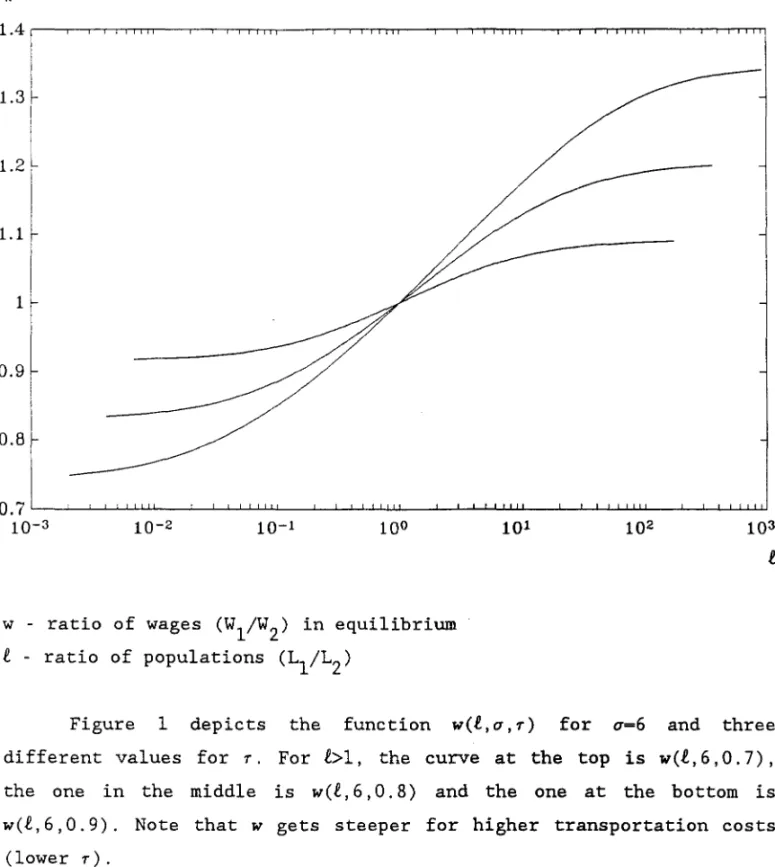
Grihfield "City Size and Place as Policy Issues".

FIGURE 1. Equilibriurn wage ratios. w 1.3 1.2 1.1 1 0.9 0.8 O.7~~-L~~~~~~~~--~~~~--~~~~~~~~~~--~~~~ 10-3 _10-2 _10-1 _10° w - ratio of wages (W 1/W2) in equilibriurn

e -

ratio of populations (L 1/L2) 101 ₁₀2 ₁₀3 t

Figure 1 depicts the function w(t,a,T) for a=6 and three

different values for T. For t>1, the curve at the top is w(t, 6, 0.7) ,

the one in the middle is w(t,6,O.8) and the one at the bottom is

w(t, 6, 0.9). Note that w gets steeper for higher transportation costs

FIGURE 2. Range of parameters for asymmetric equilibria. 1~----'---'---'---'---~---r----~---~----~----~ 0.9 0.8 0.7 0.6 0.5 0.4 0.3 0.2 0.1 O~----L---~~

____

-L~ _ _ ~ _ _ _ _ ~ _ _ _ _ ~ _ _ _ _ ~L-_ _ _ _ ~ _ _ _ _ J -_ _ _ _ ~ O 0.05 0.1 0.15 0.2 0.25 T - transportation cost

a - share of expenditures on land

Figure 2 depicts the function:

[ (l-aa)(2a-l) ll/(a-l) T(a,a)= a(a-I)+(I-a)(2a-l) 0.3 0.35 0.4 0.45 0.5 a

for four different values of a. From the l.h.s. in the picture, T(a,12) is the first to hit the x-axis, T(a,6) is the second, T(a,3) the third and T(a,2) is the last, at a=0.5.

FIGURE 3. Indirect utility ratios

u

1.15r---~---~----~~---~---_,---_r---_,---, 1.1 1.05 1 0.95 0.9 0.85 0.8L---~---~---~---~---~--~~--~--~---~ 10-4 _10-3 _10-2 _10-1 _10°

u -

ratio of indirect utilities (U1fU2)

l -

ratio of populations (L

1/L2)

101 ₁₀2 ₁₀3 ₁₀4

Figure 3 depicts the function u(l, a, a, T) for a-O .10, a=6, and

three different values for T. For

l>l,

the curve at the top is

u(l,0.10,6,0.7), the one in the midd1e is u(l,0.10,6,0.8) and the one at

•

•

FIGURE 4. Equi1ibrium ratios of popu1ations.

105~---'---'---'---r---~---.---~---~----~ " "-104 ~

~

103

~

,J

101 10°L---~ ______ ~ ____ ~L_ _ _ _ _ _ L _ _ _ _ _ _ ~ _ _ _ _ ~ _ _ _ _ ~~ _ _ _ _ _ _ L _ _ _ _ _ ~ 0.5 0.55 0.6 0.65 0.7

t -

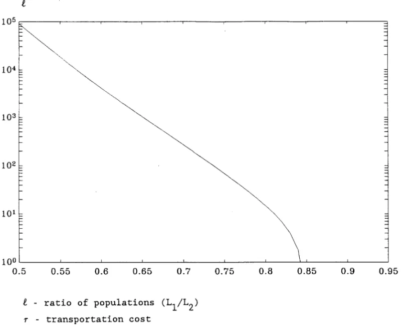
ratio of popu1ations (L₁/L₂) T - transportation cost 0.75 0.8 0.85 0.9 0.95

Figure 4 depicts the equi1ibrium ratios of popu1ations for va1ues of the parameters 0=0.10, a=6, as a function of T. Equilibrium ratios of

populations are those

t

S.t. u(t,o,a,r)=l. Note that t=l is always an equilibrium for all T, and that this is stable if and only if it is

FIGURE 5. Industry sigma labor shares for small elasticities. t 2a 0.7,---,~---,---_,---~---_T---~---_r---, 0.6 0.5 0.4 0.3 0.2 0.1 OL---~

____

~L-_ _ _ _ ~ _ _ _ _ _ _ ~ _ _ _ _ ~~~ _ _ ~~ _ _ _ _ ~~ _ _ _ _ _ _ ~ 10-4 _10-3 _10-2 _10-1 ₁₀1 ₁₀2

t

_2a industry sigma labor share in city two (L

2a/L2)

t

-

ratio of populations (L l/L2)

104

Figure 5 depicts the function 12a(t,~,a,p,r) for ~-O.5,

a-4, p-3,

and four different values of T. From the l.h.s., the first curve to hit

the x-axis is

1

2a

(t,O.5,4,3,O.9),

the second is

1

2a

(t,O.5,4,3,O.7),

the

third is

1

2a

(t,O.5,4,3,O.5),

and the last is

1

2a

(t,O.5,4,3,O.3).

The

value of

t

at which 12a(t,~,a,p,T) hits the x-axis define an upper bound for the range of equilibrium ratios of populations. At such a bound the industry with high elasticity of demand vanishes from the small city.

•

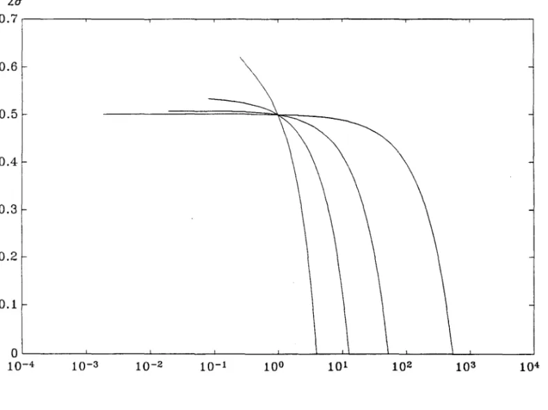
FIGURE 6. Industry sigma labor shares for high elasticities.

t

2a

1.4,---'-.-~~~---r-'-r~~'---'-~~~~--~~-r~~'---'-~~~~ 1.2 1 0.8 0.6 0.4 0.2

o

10-6 _10-3 _{10° 10}3 ₁₀6 ₁₀9

t

t

2a

-

industry sigma labor share in city two

(L

2a

/L

2

)

t

_-

ratio of populations (L

l/L2)

Figure 6 depicts the function 12a(t,~,a,p,r) for ~=O.S, 17=12,

p=8,

and four different values of

r.

From the l.h.s. , the first curve to hit the x-axis is

1

2a

(t,0.S,4,3,0.9),

the second is

1

2a

(t,O.S,4,3,O.8),

the

third is

1

2a

(t,0.S,4,3,0.7),

and the last is

1

2a

(t,0.S,4,3,0.6).

In

addition to the restriction on

t

defined by 12a(t,~,a,p,r)~0, here the restriction 12a(t,~,a,p,r)Sl is also effective for

r-O.7

and

r=O.6.

Note that here, in contrast with Figure 5, the industry sigma labor share increases for a while in city two as it gets smaller, before finally vanishing from there at

t

s.t. 12a(t,~,a,p,r)=O.

•

FIGURE 7. Equilibrium population ratios and industry concentrations (I)

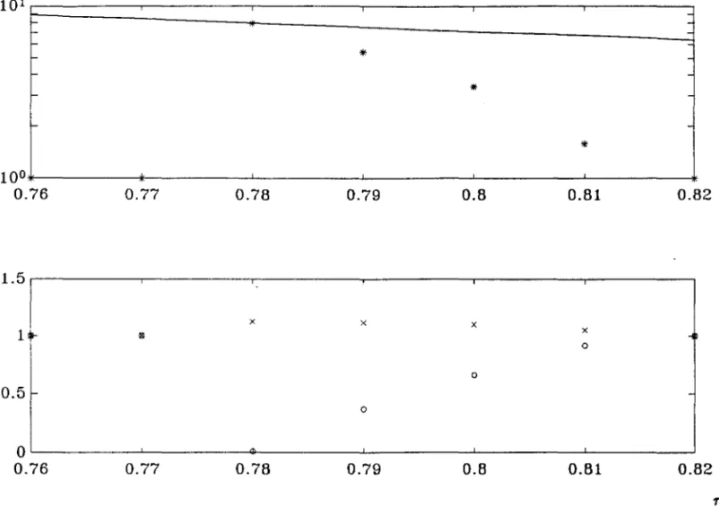
1o

1 ,---,---,---,---,---,---,

*

*

*

10°*---+---~---~---~---~---__+ 0.76 0.77 0.78 0.79 0.8 0.81 0.82 1.5r---,---r---~~---._---_.---_, 1 x x _x x o o 0.5 o OL---~---~---

__

~

________

~

________

~

________ __

0.76 0.77 0.78 0.79 0.8 0.81 0.82

*

equilibrium population ratios t (t s.t. u(t,a,~,a,p,1')=l)

population ratios t S.t. 12a(t,~,a,p,1')=0

x concentration of industry sigma in city one «Lla/Ll)/(La/L» o concentration of industry sigma in city two «L

2a/L2)/(La/L»

l'

For values of the parameters a=O .15 , ~=O. 5 , a=4, p=3, Figure 7

illustrates how equilibrium population ratios increase as l' decreases,

until it hits the upper bound. Note how the concentration of industry sigma in city two declines monotonically. Note also that if l' is toa low

there is a unique equilibrium populations ratio t-l, (for 1'-0.77 and 1'=0.76) and that it is unstable, since the utilities ratio is greater

...

oi

FIGURE 8. Equilibrium population ratios and industry concentrations (11)

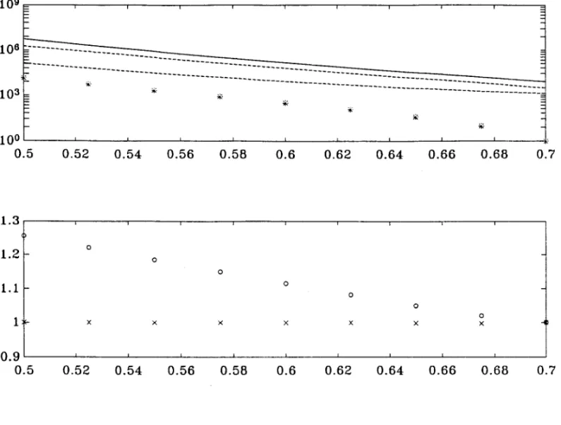
109~----'---r----~---~----~----~---~----~----~----~ E ~ I=-106

E---.~---­ F- --- ---103

E

--- ---~ ,;:. ~. 10°L---L---__ ~ ____ ~ ____ ~ ____ ~ ____ ~ ____ ~ ____ _ L _ _ _ _ _ L _ _ _ _ _* 0.5 0.52 0.54 0.56 0.58 0.6 0.62 0.64 0.66 0.68 1.3 1.2 o _o o 1.1 o _o o 1 x x x x x x o x 0.9 0.5 0.52 0.54 0.56 0.58 0.6 0.62 0.64 0.66 0.68

*

equilibrium population ratios

t (t

S.t. u(t,a,~,a,p,T)=l)

population ratios

t

S.t. 12a(t,~,a,p,T)=O

population ratios

t

S.t. 12a(t,~,a,p,T)=1

x concentration of industry sigma in city one «Lla/Ll)/(La/L» o concentration of industry sigma in city two «L

2a/L2)/(La/L» 0.7

0.7 T

For values of the parameters a=O.lO, ~=O.5, a=12,

p=8,

Figure 8 pictures progressively increasing equilibrium population ratios as T

decreases, as in Figure 7. Here though the concentration of industry sigma in city two at first increases as city two shrinks, because of the humped shape of 12a(t,~,a,p,T) for high elasticities (see Figure 6). Note that there can not be any equilibrium between the dotted lines.

. MARIO HENRIQUE SIMONSEN

N.Cham. P/EPGE SPE F825c

Autor: Franco Neto, Afonso Arinos de Me Título: City sizes and industry concentration.

086191

1111111111111111111111111111111111111111 50000

FGV -BMHS N" Pat.:F3477/98

000086191