"
-HHlOAÇAC SEiUUOVAMAS4fI'
FGV
,
SEMINAR
IO DE PESQUISA
"-ECONOMICA EPGE
Barriers to Entry and Developrnent
Arilton Teixeira
(FUCAPE)
Data
:
04/
10
/
2007(Quinta-feira)
Horário
: 16h
Local:
Praia de Botafogo, 190 - 110 andar Auditório nO 1
Barriers to Entry and Development*
Berthold Herrendorft and Arilton Teixeira
t
September 28, 2007
Abstract
Perhaps the most challenging question in development economics is why some coun-tries are so much poorer than the D.S. In this paper, we ask whether large barriers to entry are a quantitatively important reason for the income gap between the poor-est countries and the U.S. Our contribution is to develop a tractable model that captures the effects of barriers to entry and that we can use to answer this questiono We also model the other main classes of distortion typically considered in the devel-opment literature. We carry our mo deI to the data and calibrate it so as to match the main macro facts of development from the Penn World Tables. We find that this requires very large barriers to entry in the poorest countries, which account for about half of their income gap with the U.S. This suggests that if barriers to entry were tom down then the poorest countries would escape poverty.
Keywords: barriers to entry; monopoly power; rent extraction; total factor produc-tivity.
JEL classification: EOO; E04.
*This paper was initially called "Monopoly Rights Can Reduce Income Big Time". The first versions were written while Herrendorf was affiliated with the Economics Department of Universidad Carlos III de Madrid, Spain. We are grateful to Edward Prescott, Richard Rogerson, and James Schmitz for their help and encouragement. We have benefited from the comments and suggestions of Yan Bai, Michele Boldrin, Marco Celentani, Juan Carlos Conesa, Antonia Díaz, Ronald Edwards, Fernando Garcia-Belenguer, Thomas Holmes, Belén Jerez, Gueorgui Kambourov, Pete Klenow, John McDowell, Stephen Parente, B. Ravikumar, José-Victor Ríos-Rull, Michele Tertilt, and Ákos Valentinyi. Moreover, we have received useful comments at the ASSA Meetings in San Diego, ASU, the Federal Reserve Banks in Atlanta, Dallas, and Minneapolis, Edinburgh, Foundation Gestulio Vargas, Iowa, the SED Meetings in Paris and Florence, SITE (Stanford), Southampton, UCLA, UC Riverside, and the Vigo-vVorkshop in Dynamic Macro. Herrendorf acknowledges research funding from the Spanish Dirección General de Investigación (Grant BEC2000-0170) and from the Instituto Flores Lemus (Universidad Carlos lII).
tDepartment of Economics, ~T.P. Carey School of Business, Arizona State University, Tempe, AZ 85287-3806, USA. Email: [email protected]
tFundacao Capixaba de Pesquisa, Av Saturnino Rnagel Mauro, 245 Vitoria, ES 29062-030 Brazil. Email: [email protected]
1
Introd uction
Perhaps the most challenging question in development econOE .; is why some countries are so much poorer than the V.S. In their classic book, North and Thomas (1973) ar-gued that barriers to entry prevent the development of poor countries because they give monopoly power to groups of individuaIs that would lose economic rents if better tech-nologies and more productive working arrangements were adopted. These insider groups protect their rents by blocking the adoption of better technologies and more productive working arrangements, thereby preventing development.1 Holmes and Schmitz Jr. (1995),
Parente and Prescott (1999), Acemoglu (2005), and Herrendorf and Teixeira (2005) de-veloped this idea further. In this paper, we ask whether large barriers to entry are a quantitatively important reason for the income gap between the poorest countries and the U.S.
The evidence on the existence of barriers to entry in poor countries goes back at least to de Soto (1989). He documented that Peru had large barriers to starting a formal business and argued that this was a big reason for its poverty. Building on de Soto's work, Djankov et aI. (2002) measured barriers to starting a formal business for a sample of 85 countries during 1997. They found that the developing countries of their sample had much larger barriers to starting a formal business than the developed ones. There is also some evidence on the detrimental effects of barriers to entry. To begin with, using a sample of OECD countries, Alesina et aI. (2003) found that product market regulation is negatively related to investment and Nicoletti and Scarpetta (2003) found that it is negatively related to TFP. In both studies barriers to entry turn out to be the dimension of product market regulation that has the biggest negative impacto Industry case studies are another source of evidence on the detrimental effects of barriers to entry, documenting cases mostly from rich countries in which reductions in barriers to entry - and the implied increases in competition - raised labor productivity or TFP; see Clark (1987), Wolcott 1 Lindbeck and Snower (2001) define insiders as incumbent workers that enjoy more favorable employ -ment opportunities than others (the outsiders), on account of labor turnover costs. Here we use insiders more generally to refer to individuais that are shielded fram outsider competition by entry barriers.
.. "
(1994), McKinsey-Global-Institute (1999), Holmes and Schmitz (2001a,b), Parente and Prescott (2000), Galdon-Sanchez and Schmitz Jr. (2002), Lewis (2004), and Schmitz Jr. (2005). In sum, there is evidence that barriers to entry are much larger in poor countries but exist also in rich countries. There is also evidence - mostly from rich countries - that barriers to entry are harmful. What is missing is evidence from poor countries about how harmful they are there.
Our contribution in this paper is to develop a tractable model that captures the main effects of barriers to entry and that we can carry to the data to answer our question whether barriers to entry are a quantitatively important reason for poverty. We start with a standard development model that splits the aggregate economy into an agricul-tural sector and many nonagriculture sectors ("manufacturing"). The agricultural sectar produces agricultural consumption and the nonagricultural sectors produce manufactured consumption, intermediate goods, and capital. The agricultural sector uses the usual in-puts land and labor along with intermediate inputs and capital from manufacturing. Since land is in fixed supply, the agricultural technology has decreasing returns to the reproducible factars. Preferences are such that the income elasticity of agricultural con-sumption is less than one ("Engel's Law").
The novelty of our work is to introduce barriers to entry and rent extraction by insider groups into this model. We follow the development literature, e.g. Parente and Prescott (1999), and assume that barriers apply to entry into manufacturing whereas entry into agriculture is free. The reasoning behind this assumption is that many agricultural goods can be produced through subsistence farming, which makes it hard to erect barriers and establish monopoly power in the agricultural sectar. We also assume that insider groups in the manufacturing sectors can choose the technologies ar working arrangements, and that they can extract rents by deliberately choosing inefficient technologies or working arrangements. Solving the rent-extraction problem of the insider groups is challenging here because each group needs to take into account how the capital stock in its sector reacts to its choice of technology ar working arrangements. In other words, the problem
of each insider group is dynamic here. We characterize the solution to this problem and
show that larger barriers to entry reduce total factor prodw::tivity (TFP henceforth) and
the capital-labor ratio. This is consistent with the evidence reported by Nicoletti and Scarpetta (2003) and Alesina et aI. (2003). To our knowledge, we are the first to construct a model that qualitatively accounts for this evidence.
Most of the development literature has studied distortions other than barriers to
entry.2 We argue that we can capture the effects of these other distortions by higher taxes,
by lower agricultural TFP, and by lower efficiency units of labor, all compared to the U.S. We define taxes broadly to include actual taxes, but also bribes, side payments, and the
like.3 Reasons for lower agricultural TFP include less fertile farm land, worse climate, or less developed transportation systems.4 Lower efficiency units of labor capture lower
endowments of human capital but also the time lost dealing with inefficient bureaucracies,
overwhelming regulation, and similar obstacles.
To take this model to the data, we identify the U.S. with the undistorted model
economy, for which we use off-the-shelf parameter values to the extent possible. We then choose the sizes of barriers to entry and of the other three classes of distortions so as to match quantitatively the cross-sectional variation in the main macro statistics of development reported by the Penn World Tables 96 (PWT96 henceforth). A qualitative
summary of these statistics is as follows: poor countries have larger shares of the workforce
in agriculture than rich countries, larger shares of agricultural goods in consumption,
smaller shares of investment in output, and higher relative prices of investment goods
and food.
We find that matching these macro-facts of development requires very large barriers
to entry in the poorest countries, which account for about half of their income gap with
the U.S. Moreover, there are relatively large taxes and low efficiency units of labor in these
countries, which each account for around twenty percent of the observed cross-:-country
2 A recent exam pIe is Rsieh anel KIenow (2007).
3See Restuccia anel Urrutia (2001) anel Herrenelorf anel VaIentinyi (2006) for further eliscussion.
"
...
differences in income. Agricultural TFP in the poorest countries is also considerably lower than in the U.S. but this leads to income differences of less than five percent only. In sum, we find that large barriers to entry are the most important reason for why some countries are so poor. Our finding that cross-country differences in the efficiency units of labor account for around twenty percent of the income gap with the U.S. is elose to what
development-accounting studies find about cross-country diflerences in human capital; see e.g. Hall and Jones (1999), Hendricks (2002), and 7. This is remarkable because our
calibration strategy does not use any information about cross-country differences in years of schooling, from which these studies construct their measures of human capital.
Although we have not directly targeted this, our calibrated model also predicts that the cross-country labor productivity gap in agriculture is many times the gap in
nona-griculture. This is consistent with the evidence from the development literature that the problem of poor countries lies in their agricultural sectors.5 Importantly, our model delivers this although the most important distortion - barriers to entry - applies to
nona-griculture. The main reason for this is that barriers increase the relative prices of both intermediate goods and capital, which drastically decreases the use of these two factors
of production in agriculture.6
Our papel' contributes to the recent development literature that offers theories of
cross-country differences in TFP and income. Examples inelude Holmes and Schmitz
Jr. (1995), Stokey (1995), Parente and Prescott (1999), Acemoglu and Robinson (2000),
Acemoglu and Zilibotti (2001), Restuccia and Rogerson (2003), Amaral and Quintin (2004), Herrendorf and Teixeira (2005), and Erosa and Hidalgo (2007). The variety of possible ways in which distortions can affect TFP and income suggests that there are several, not just one, answers to the question why are some countries are so much poorer
than the U.S. Here we establish that large barriers to entry are a major distortion that must not be ignored .
5Some cJassic references are Schultz (1964), Ruttan and Hayami (1970), and Kuznets (1971). Recent references are Caselli (Forthcoming: 2005) and Restuccia et al. (2006).
6 A similar propagation mechanism is present in the work of Schmitz (2001) about government
ineffi-ciencies in investment production.
Since barriers to entry lead to monopoly power of the insider groups, our work also contributes to the literature on the cost of monopoly. Harberger (1954) argued that this
cost is small if monopoly just increases the price and reduces the quantity. While Laitner (1982) subsequently pointed out that the cost of monopoly can be larger when there is capital, he still estimated it to be a few percentage points of GDP only. More recently,
Parente and Prescott (1999) argued that monopoly can be much more detrimental if it
also decreases TFP. Our work goes beyond Parente and Prescott (1999) in two crucial
dimensions. First, we model the interaction between monopoly and capital accumulation
whereas they used a static model without capital accumulation. vVhile abstracting from
capital accumulation simplifies matters, it does shut down an important channel through which the detrimental effects of monopoly get propagated to the whole economy. Second, except for barriers to entry and the other classes of distortions, we have written down
a standard development model with capital that we can carry to the data and use to
measure the costs of the monopoly power implied by barriers to entry. In contrast, the model of Parente and Prescott (1999) does not naturally lend itself to measurement.
The next section lays out the environment and section 3 defines the equilibrium. In
section 4, we show existence and uniqueness of equilibrium and characterize the differences between the equilibrium of the undistorted and the equilibrium of the distorted economy.
Section 5 describes our calibration and reports findings. We conclude with a discussion of our modeling assumptions in section 6. An Appendix contains all proofs.
2
Environment
Time t is discrete and there is no uncertainty. The economy is populated by a measure one of households, which have identical preferences over sequences of an agricultural and a manufactured consumption good. We represent preferences by a time-separable
"1 non-homothetic utility functions:
;:
~
f3
E (0,1) is the discount factor, Ca and em are the consumption of the agricultural and the manufactured good, and ex E (O, 1) is a relative weight. The positive constant-º
implies that the income elasticity of agricultural consumption will be smaller than oneand Engel's Law will hold.
In each period households are endowed with one unit of labor. In the initial period
they are also endowed with equal shares l of the total available land and with strictly positive quantities bo of capital. Capital depreciates at rate {) E (0,1).
There are three final goods sectors, which produce agricultural consumption, ma nu-factured consumption, and investment. There is also a continuum of sectors j E [O, 1]
that produce intermediate inputs for the final good sectors. We will refer to the first
sector as agriculture and to all remaining sectors as manufacturing. While the two final manufacturing sectors use intermediate inputs only, the agricultural sector uses also ca p-ital, land, and labor. The intermediate good sectors themselves use capital and labor but no other intermediate goods.
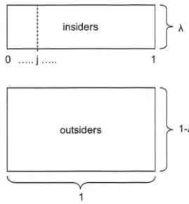
Households differ in their type. A measure 1 - À are outsiders, which are all identical.
A measure À E (0,1) are insiders in one of the intermediate good sectors j E [0,1]. The density over the insiders of the different intermediate good sectors is uniform. In
other words, there are equalIy many insiders in alI intermediate-good sectors. Figure 1 illustrates the resulting distribution of household types. The type determines where the
household can use its labor endowment. The insiders oftype j E (0,1) can transform their labor endowment into insider labor services in intermediate good sector j and into labor services in agriculture. Each outsider can transform his labor endowment into outsider labor services in any intermediate good sector and into labor services in agriculture.
ote that for simplicity we do not alIow the insiders of type j to transform their labor
endowment into outsider labor services in other intermediate good sectors n =1= j. Note
Figure 1: The household types insiders } À L T
-o
...
j ... outsiders 1-À ~~---~ V ~---~/ 1too that for simplicity all households have the same endowments of labor and land, so only the physical capital endowment may depend on the household type.
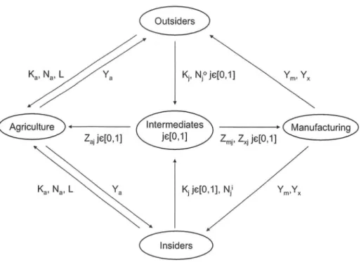
Before we specify the technologies, we summarize the key features of our environment in Figure 2. The figure illustrates that all households rent capital, Ka, labor Na, and land, L, to the agricultural sector and capital, Kj, to the intermediate good sectors. The
difference between outsiders and insiders is that the outsiders rent outsider labor,
Nr,
to all intermediate good sectors whereas the insiders rent insider labor,
Nj,
only to their intermediate good sector. All households purchase agricultural consumption goods, Ya, from agriculture and manufactured consumption goods,Y;n
,
and investment goods, Yx,
from final manufacturing. The intermediate good sectors sell intermediate inputs Zaj to agriculture and Zmj and Zxj to the final manufacturing sectors.We now specify the different technologies. All technologies have constant returns and in each sector there is a stand-in firm that behaves competitively. The agricultural sector produces according to:
where Z. -
(1'
Z.j.
~
'
dj).~,
(1)o
.
"
Figure 2: Environment
Ym, Yx
Zmi' ZXi je:[O, 1]
Aa is agricultural TFP and 'IjJ E (O, 1] are the efficiency units of labor per unit of labor
rented. Bk, BI, Bn, Bz E (0,1) are the share parameters of capital, land, labor, and interme
-diate inputs. Constant returns require Bk
+
BI+
Bn+
Bz=
1. The elasticity of substitutionbetween the intermediate goods is denoted by (J".
The final manufacturing sectors produce according to:
Ax
is the TFP of producing investment goods from intermediate goods.Each intermediate good can be produced with a technology that uses capital and insider labor only and a technology that uses capital and outsider labor. We indicate
the two technologies by the superscripts i and o, so
Z]
andZJ
are the quantities ofintermediate good j produced with insider and outsider labor. The technologies are:
Z;
= Aj(K;)B('ljJNJ)l-B,Zj
= AO(Kj)B('ljJNj)l-B.(2a)
(2b)
A; is specific to the insider technology in intermediate good sector j whereas AO applies
to all outsider technologies. The use of intermediate inputs in the final good sectors may
not exceed the sum of the intermediate goods produced with both technologies:
We follow the development literature and consider tax distortions as a possible source of relative price variation. We lump sum rebate the tax revenues to the households. Taxes are broadly defined as any distortions that increases a goods price and that leads to income for some agents. Examples are value-added taxes, tariffs, bribes, and rents from monopoly power other than those accruing in the labor markets of the intermediate
good sectors. Since we have three final goods and since we rebate the tax revenues, it is
sufficient to consider the two final-goods taxes Ta on agricultural consumption and Tx on investment. We also consider a tax Tz on intermediates used in agriculture.
We finish the description of the environment with the market structure. Trade takes place in sequential markets. In each period there are markets for both consumption goods, the investment good, capital, land, outsider labor, each type of insider labor, and each intermediate good.
3
Equilibrium Definition
We distinguish between an undistorted and a distorted version of our model economy. We normalize Aa = 1 for the undistorted economy and restrict Aa ::; 1 for the distorted
economy. We denote by A the largest possible value of A; and AO.
. ..,
If 'l/J = Aa = 1, AO = A, and Ta = Tx = Tz = O the model economy is undistorted and
the insider and outsider technologies are identical. Household types then are just names
that do not have any consequences for equilibrium prices or quantities. We set A}
=
Ain this case.
If 'l/J,Aa E (0,1], AO E (O,A), and Ta,Tx,Tz E (- 00,00), then our model economy is distorted. The primitive 'l/J captures everything that reduces the efficiency units of labor that get supplied vvhen households work for unit of time. This includes not only the effects of lower human capital endowments but also those of inefficient bureaucracies
or overwhelming regulation. The primitive Aa summarizes everything that makes ag
ri-culture less efficient, for example less fertile farm land, worse climate, or less developed
transportation systems.7
The primitive AO summarizes the barriers that outsiders face when they enter the
nonagricultural sectors. We express them as a share of output instead of a fixed entry cost
because this maintains constant returns.8 Note that entry barriers apply when households
want to leave agriculture and enter nonagriculture. The reason is that most agricultural goods are easily produced in the unofficial economy 01' in subsistence farming. This should make it hard to erect barriers and establish monopoly power in the agriculture sector.
There are different interpretations for
AO.
Caselli and Coleman (2001) argue that workingin nonagricultural requires a minimum degree of human capital (e.g. literacy) that is not
required in agriculture. Since we have assumed that all households in an economy have
the same 'ljJ, AO picks up that the outsiders may be less educated than the insiders, and
so they may have a lower marginal product in nonagriculture. Second, as discussed in
the introduction, poor countries are plagued by many formal and informal barriers to
entry. For example, de Soto (1989) gives a detailed account of the mindboggling variety of administrative steps and bureaucratic procedures required to start a formal business in Peru. In addition, there are accounts of many informal barriers to entry. They often ... 7See Herrendorf et ai. (2007) on transportation and agricultural productivity.
8This could be derived in a more disaggregate environment where the outsiders pay a fixed cost to start operating a decreasing-returns-to-scale technology in an intermediate good sector.
result from the preferential treatment of insiders, for example in the form of subsidized credito
We assume that the insiders of each intermediate good sector can exploit the monopoly power resulting from the entry barriers by acting as a group: in each period the group of insiders of type j collectively chooses next period's TFP for its insider technology,
A;'
E [O,Al.
This choice happens simultaneously with the other decisions. As Holmes and Schmitz Jr. (1995) and paJ'ente and Prescott (1999), we assume away problems of coordination or free riding.The choices of each insider group are strategic at the sector leveI in that it takes into account how its TFP choice affects the relative price of its intermediate good, the capital and labor allocated to its sector, and the consumption and investment choices of its members. In contrast, the insider groups take as given all aggregate vaJ·iables. In other words, each insider group is large in its intermediate-good sector but small with respect to the rest of the economy.
Before we go into the details of our equilibrium concept we sketch its broad features.
Since the different insiders, outsiders, and in si der groups each solve identical problems, we focus on symmetric equilibrium. We also focus on recursive equilibrium in which all deci -sion makers condition their actions in each period only on the observable state variables.
Moreover, except for the choices of the insider groups, all agents behave competitively.
We start with the description of the state variables.9 Since we focus on symmetric equilibrium, all intermediate good sectors, insider types, and outsider types will each have
the same equilibrium allocations. We therefore simplify our notation and drop the sector
index j. We denote individual state variables by lower-case letters: bi and bO are the
capital holdings of a particular insider and a particular outsider. We denote sector-wide state variables by upper case letters: the insider TFP of a particular intermediate good
sector is Ai and the capital holdings of the other insiders of this sector are Bi. We denote
economy-wide state variables by upper-case calligraphic letters: Ai is the insider TFP
9The following material draws 011 Teixeira (1999).·
"
".
in the other sectors, Bi are the capital holdings of the insiders in the other sectors, and
BO
are the capital holdings of the other outsiders.In sum, the individual state is
(bi
,
bO),
the sector-wide state is(A
i
,
Bi),
and the economy-wide state is(Ai
,
Bi
,
BO).
The laws of motions of the sector-wide and theeconomy-wide states are given by:
To economize on the notation, we abbreviate some state variables: S
V\Te choose manufactured consumption as the numeraire. The relative prices of agri-cultural goods and capital and the rental prices of outsider labor, capital, and land are
functions of the aggregate state only: Pa(S), Px(S), WO(S), 1'k(S), and 1'l(S). The relative
price of a particular intermediate good and the rental price of a particular type of insider
labor depend aIs o on the insider TFP in the corresponding intermediate good sector:
V\Te now describe the households' problems. Recall that households can invest in any sector of the economy irrespective of whether they work there or noto Consequently the capital stock that the insiders own differs in general from the capital stock with which they produce. To emphasize this we have represented the two different capital stocks by
the different symbols Bi and Ki.
A particular outsider chooses his current consumption and future capital stock, taking as given the economy-wide state S, the corresponding law ofmotion
9,
and his own capital(3)
S' = 9(S),
where VO denotes his value function and
TO(S)
denotes the lump sum tax rebate to each outsider. The solution to this problem implies the outsider policy function (c~, c~, bOI)A particular insider chooses his current consumption and future capital stock, taking as given the economy-wide state S, the corresponding law of motion 9, its sector's state 5, the corresponding law of motion G, and his own capital stock bi:
(4) S.t. (1
+
Ta)Pa(S)c~+
c~+
(1+
T
x)Px(
S)W '
-
(1 -8)b
i]= rk(S)bi
+
wi(S, Ai)+
rl(S)l+
T
i(
S
),
(S, 5) I
=
(G(S), G(S, 5)),where Ti(S) denotes the lump sum tax rebate to each insider. The solution to this problem implies the insider policy function (c~, c~, bi/)(S, 5, bi
).
We continue with the problem of each insider group. Recall that while it takes all
aggregate price functions and laws of motion as given, it takes into account how its TFP choice affects the relative price of its intermediate good, the capital and labor used with its insider tpchnology, and the consumption and investment choices of its meml '. So, it chooses Ail
so as to maximize the indirect utility of its members plus the contllluation
lONote that to economize on notation we have omitted profits. This is without 10ss of generality
value, taking as given the economy-wide state S, the corresponding law of motion
g,
the sector-wide state S, and the law of motion of the sector-wide insider capital, G2:(5)
S.t. (S, Si) /
=
(G(S), G2(S, S)).A solution to this problem implies the policy function A i' (S, S).
We now turn to the sector allocation functions. All input factors and production
quantities except for those of the intermediate good sector depend just on the aggregate state S: (Ya, Ka, L, Na, Za,)(S), (Ym, Zm)(S), (Yx, Zx)(S). Those of the intermediate good sector depend also 011 insider TFP Ai: (Zi, Ki, N i, ZO, KO, N°)(S, Ai). Listing the supplies of the different goods on the left-hand sides and the demands on the right-hand sides,
market clearing requires:
Ya(S)
=
(1 - À) C~(S, bO)+
À c~(S, S, bi ), (6a) Y;n(S) = (1 - À) c~(S, bO)+
À C!n(S, S, bi ), (6b)Yx(S)
=
(1 - À) bO/(S, bO)+
À bi/(S, S, bi ) - (1 - 6)[(1 - À) bO+
À bt (6c) Zi(S, Ai)+
ZO(S, Ai) = Za(S)+
Zm(S)+
Zx(S), (6d)(
1 -
À) bO+
À bi=
Ka(S)+
KO(S, Ai)+
Ki(S, Ai),(6e)
1 - Ni(S, Ai) - N°(S, Ai) = Na(S),
(1 - À)l
+
Àl=
l=
L(S).(6f)
(6g) (6h)
The first three conditions require that the markets for the two consumption goods and
for investment clear. The fourth condition requires that the market for a particular intermediate good clears, and the fifth condition requires that the market for capital
clears. The next two conditions require that the markets for the different types of labor
clear. The last condition requires that the market for land clears.u
Several consistence requirements have to hold in equilibrium. To begin with, the
economy-wide states, the sector-wide states, and the in 'lVidual states need to be cons
is-tent with each other:
(7a)
(7b)
(7c)
The laws of motion that the decision makers take as given when they make their choice
need to be consistent with their policy functions:
91(S) = G1(S,Ai,Si)
=
Ai'(S,Ai,Si), 92(S) = G2(S, Ai, Si)=
bi'(S, Ai,s
i,
Si), 93(S) = bO'(S, SO). (7d)(7e)
(7f)Moreover the value function of the insider group needs to consistent with the value func
-tion of the particular insider:
(7g)
Finally the lump sum rebates need to equal the tax revenues:
TO(S) = TzPz(S)Za(S)
+
TaPa(S)c~(S, SO)+
TxPx(S)W'(S, SO) - (1 - c5)b°], (7h)Ti(S) = TzPz(S)Za(S)
+
TaPa(S)C~(S, Ai, Si, Si)+
TxPx(S)W'(S, Ai, Si, Si) - (1 - c5)biJ.
(7i)11 Note that in symmetric equilibrium we can drop the integraIs. Note too that we have abstracted
from borrowing and lending between insiders and outsiders. This is without loss of generality because
below we focus attention on steady state equilibrium.
!"
.
.
.
;.
Definition 1 (Equilibrium in the undistorted economy) Given Ai
=
Ai=
AO=
A, 'IjJ
=
Aa=
1, and Ta=
Tx=
Tz= O
, an equilibrium in the undistorted economy is-
laws
of motion
(Ç
,
G)
- value functions Vo, Vi
l"
f
t"(0
°
bOI)(i i
bil )- po ~cy unc wns ca, cm' , ca' cm' such that:
- all production factors are paid their marginal products - the value functions satisfy (3)-(4)
- the policy functions solve (3)-(4) - the market clearing conditions
(6)
hold - the consistency requirements (7) are satisfied.Definition 2 (Equilibrium in the distorted economy) Given AO E
(O,
A),'l/J,
Aa E(0,1], and Ta, Tx , Tz E
(-
00,00),
an equilibrium in the distorted economy is- tax rebate functions TO, Ti
- sector allocationfunctions (Ya, J(a, L, Na, Za), (Ym, Zm), (Yx, Zx), (Zi, J(i, Ni , ZO, J(0, N°) - laws of motion (9, G)
- value functions Vo, Vi, Vi
l "
f
t"(0
°
bO ')(
i i
bi ') Ai I- po ~cy unc wns ca, cm' , ca, cm' ,
such that:
- if a production factor is used in a sector, then it is paid its marginal value product; if a
"
production factor is not used in a sector, then its marginal value product does not exceed its rental rate;
- the value functions satisfy (3)-(5)
- the policy functions solve (3)-(5)
- the market clearing conditions
(6)
hold- the consistency requirements (7) are satisfied.
4
Steady State Equilibrium: Existence, U niqueness,
and Characterization
We now show the existence and uniqueness of the steady-state equilibria in both economies and we characterize the differences between them. Since our utility function features a subsistence leveI of agricultural consumption ,º, existence of equilibrium requires that the agricultural sector can produce this subsistence level. Conditions (22a) and (24b) in the appendix ensure this for the undistorted and distorted economy, respectively.
Proposition 1 (Steady-state equilibrium in the undistorted economy)
Let Ai = Ai = AO = A be such that condition (22a) in the appendix is satisfied. Then
there exists a unique steady state equilibrium.
Proof. See Appendix A.2.
In the distorted economy existence of steady-state equilibrium also requires that the insider groups are not too large and the upper bound A on the insider productivity is not
too small. The two inequalities of (24c) in the appendix ensure that this is the case.
Proposition 2 (Steady-state equilibrium in the distorted economy)
Let (J E (0,1), AO E (O, A] and ('lj!, Aa, À, A, Ta, Tx, Tz) be such that conditions (24b) and (24c) in the appendix are satisfied.
• There exists a uni que steady state equilibrium.
• In the steady-state equilibrium the insiders work only in their intermediate good
sectors, and they strictly prefer this; the outsiders work only in agriculture, and
they are indifferent between this and working in the intermediate good sectors.
• The steady-state equilibrium value of Ai lies in [AO,
AL
and it decreases if AOde-creases or À increases.
Proof. See Appendix A.3.
To gain intuition for these results, it may be useful to consider for a moment a monop-olist producer in an intermediate sector, instead of a group of insiders. Such a monopolist would increase the relative price of the intermediate good above the competitive one so
as to restrict production. Demand is inelastic here, a E (O, 1), so he would increase the relative price until potential entrants are just indifferent between entering and staying
out. The difference with an insider group is that it cannot directly choose a higher
rela-tive price of the intermeeliate gooel it produces because that price is eletermined by the
competitive firms. However, the insieler group can indirectly choose a higher relative price
by choosing lower TFP. With inelastic elemanel for intermediate goods, this increases the relative price by more than it decreases the insiders' marginal product, so it increases the
real insider marginal value product.
An insider groups' monopoly power is limited by the possible entry of outsielers into its intermediate goods sector. If outsiders enter, then the relative price must be such
that the outsider marginal value product is the same in the intermeeliate gooel sector
and in agriculture. Choosing an even lower TFP then decreases the marginal insider
product, but it does not affect the relative price anymore. So, choosing an even lower
TFP then decreases the insider marginal value product and makes the insider group worse
off. Taking these two arguments together it follows that the insider groups choose Ai! such that the outsiders are just indifferent between entering the intermeeliate good sector
anel staying out.
We can also provide some intuition for the comparative static results of proposition
2. To begin with, the lower is AO the larger is the relative price of intermediate gooels that makes the outsiders indifferent between working in agriculture and the intermeeli
ate-good sector. Since choosing a lower Ai! increases Pi as long as the outsielers strictly prefer
agriculture, a lower AO makes choosing a lower Ai! optimal. Turning to the comparative 18
statics of the grou size, larger insider groups can produce a given demand for their
prod-uct with lower A ~o a larger .À decreases the optimal A i'. Note that these arguments
are related to the !lecessary conditions for existence, (24c), which require that A is large
enough and À is not too large. The first condition ensures that the insider groups can
satisfy the demand for their product when they choose Ai = A and the second condition
ensures that the insiders do not produce more than the demand for their product when
they choose Ai = AO.
The result that larger barriers to entry (a smaller AO) reduce the TFP of the
intermedi-ate goods sectors is consistent with a large body of evidence. To begin with Nicoletti and
Scarpetta (2003) found that product market regulation is negatively related to TFP in a
panel of OECD countries. Importantly, barriers to entry are the most crucial element of
product market regulation. Moreover, Nickell (1996) found that more competition in UK
sector led to higher TFP growth. Finally, many industry case studies for developed and
developing countries found that more competition increase labor productivity and TFP;
see for example Clark (1987), Wolcott (1994), McKinsey-Global-Institute (1999), Holmes
and Schmitz (2001a,b), Parente and Prescott (2000), Galdon-Sanchez and Schmitz
Jr.
(2002), Lewis (2004), and Schmitz Jr. (2005).
For the quantitative work that follows it is important to realize that entry barriers
and rent extraction do not only have a direct effect on the TFP of the intermediate good
sectors but also important indirect effects. The first one works through the capital-labor
ratios in the intermediate good sectors. Equation (14e) of Appendix A.l shows that the
capital-labor ratios in the intermediate good sectors decrease in Ai:
(8a)
Since Ai del..reases when AO decreases larger barriers imply a lower capital-labor ratio
in the intermediate good sectors. The second indirect effect works through the relative
prices of capital and intermediate goods on agriculture's use of these two input factors.
Larger barriers increase these relative prices, which reduces the capital-labor ratio and
..
~.
the intermediates-labor ratio in agriculture. Equations (16b) and (16c) of Appendix A.l show this formalIy:
(8b)
(8c)
Putting (8a) and (8b) together, we obtain an expression for the aggregate capital-labor
ratio in the distorted economy, which also decreases when
AO
decreases:In sum larger barriers (a smalIer value of
AO)
reduce the capital-labor ratio in alI sectorsand on the aggregate. This is consistent with the evidence reported by Alesina et al.
(2003). A similar propagation mechanism is present in the work of Schmitz (2001), who
argued that if the government produces investment goods inefficiently, then this reduces
the labor productivity of all sectors that use these investment goods. Schmitz found
sizeable effects on income of around a factor 3.
5
Quantitative Analysis
5.1
Calibration
We calibrate our model economy by mapping the undistorted economy into the D.S.
economy. We choose to do this because the D.S. economy has relatively smalI distortions
and is the biggest and most studied developed economy. We map the distorted economy
into the aggregate of the 34 poorest countries in the 1996 Benchmark Data of the Penn
World Tables (PWT96 henceforth). We choose these 34 countries because the poorest 25% of the sample population live in them.12 Vve aggregate over these 34 countries instead
12From poorest to richest, they are: Tanzania, lVlalawi, Yemen, Madagascar, Zambia, Mali, Tajikistan,
Nigeria, Benin, Sierra, Leone, Mongolia, Kenya, Congo, Bangladesh, Nepal, Senegal, Vietnam, Pakistan,
calibrating om model country by country because we will use data from two different some' ;, namely 1 fIe P\iVT96 and the FAO. Unfortunately the FAO data is only available
for 24 of the 34 poorest countries of the PWT96.
Table 1:
Individually
calibrated parameters(3 B l PC l us
0.94 0.06 0.33 0.13 0.14 0.26 0.47 1.32 2.2 0.36 0.44 1.44
We start with the model parameters for which off-the-shelf values are available. We follow Cooley and Prescott (1995) and set (3
= 0.95
and {)=
0.06. We use the parameter values of? for the U.S. factor shares in sector gross output: B = 0.33, Bk = 0.13, Bl = 0.14, Bn=
0.26, Bz=
0.47.We continue with parameter values that we calibrate individually. \iVith regards to Ax and Tx, we use that Px = l/Ax in the undistorted model economy and Px
=
(1+
Tx)/Ax in the distorted model economy. In the PWT96 the price of investment relative to manufactme consumption equals 0.76 for the U.S. and 2.4 for the poor country. Thus we set Ax=
1.3 and Tx=
2.2. \iVe calibrate the land endowments, l, and the size of the insider groups, À, from data provided by the Food and Agricultural Organization (2004), which is available for the 24 of the 34 poorest countries of the P\~TT96. Aggregating over these 24 countries, we find for the poor country that the ratio of arable land to the active population is 0.44 and the share of the active population in agricultme is 64%. Recalling that the total active population has measure one in our model, we therefore setÀ
=
1 -Nt
C=
0.36 and lPC=
0.44. Following a similar logic, we set ZUS = 1.4 for the D.S. Table 1 summarizes the parameter values that we calibrate individually.\Me have eight more parameters to calibrate: ex, f, 'ljJ, A, AO, Aa, Ta, Tz.13 Our strategy is to choose them so as to match the following eight development facts from the P\lVT96: the income difference between the U.S. and the poor country; the shares of agricultural Cote d'Ivoire, Cameroon, Moldova, Azerbaijan, Bolivia, Uzbekistan, Kyrgyzstan, Armenia, Guinea, Syria, Sri Lanka, and Albania.
13Recall that we normalized Aa = 1 for the undistorted economy.
.,
.
.
.
....i
'
~
.
'
~
...
Table 2: Jointly calibrated parameters
a
º
'IjJA
AO
Aa
T
a
T
z
0.09 0.004 0.52 0.25 0.04 0.32 0.24 1.5
consumption in total consumption measured in international dollars in the poor country
and the V.S.; the shares of investment in GDP measured in international dollars in the poor country and the U.S.; the share of the active population in agriculture in the U.S.;
the domestic relative prices of agriculture in the U.S. and in the poor country. Note that
since we match the relative prices in the U.S., units in our mo deI are equal to those in
the P\iVT96. Consequently, we can use the international relative prices from the PWT96
when we evaluate model quantities in international prices.
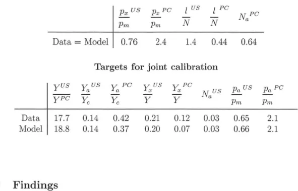
Table 3 summarizes the values of our targets.14 The first part refers to targets that
we use for the individual calibration and the second part refers to targets that we use
for the joint calibration. We can see the common regularities: the poor country has a
much larger share of agricultural consumption, a much smaller share of investment, and larger relative prices of agricultural goods and investment. Except for the cross-country
difference in the relative price of agricultural goods, these regularities are well known; see
for example Reston and Summers (1988), Easterly (1993), Jones (1994), Restuccia and
U rrutia (2001), and Rerrendorf and Valentinyi (2006).
vVe conduct a grid search and choose the parameter values that minimize the perce
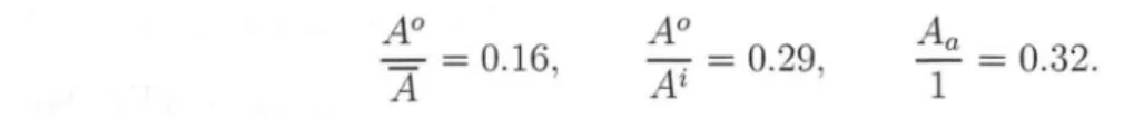
nt-age difference between the eight target values in the data and the model. Table 2 reports the calibrated parameter values. We should mention that the calibration implies that the insiders choose a smaller value of Ai than possible: Ai
=
0.14. To put the calibrationresults into perspective, note that
AO
A
=
0.16,AO
Ai=
0.29,-
Aa
=
0.32.1
14We should mention that Yc stands for total consumption in international prices.
We can see that outsider TFP in the intermediate-good sectors is 16 percent of the
maximum possible TFP. Moreover, if the outsider entered, then they would produce with
29 percent of the insider TFP. In other words, there are large barriers to entry in the
distorted economy. There are also large taxes in the poor country: more than 20% on
agricultural output, 150% on intermediate inputs to agriculture, and more than 200% on
investment goods. Furthermore, the agricultural TFP of the distorted economy is four
percent of that in the undistorted economy and the efficiency units of labor are about
half of those in the undistorted economy. The large differences between the undistorted
and the distorted economy suggest that all of four distortion may play an important role
in accounting for the income difference between the D.S. and the poor country. In the
next subsection, we will explore how large their roles are.
Table 3: Targets for individual calibration (PC for poor country)
Px us Px PC l us l PC
N PC
N N a
Pm Pm
Data = Model 0.76 2.4 1.4 0.44 0.64
Targets for joint calibration
y US Yaus y PC Y us Y xPC NUS Pa us Pa PC a x - - - -ypc
Yc
Yc Y Y a Pm Pm Data 17.7 0.14 0.42 0.21 0.12 0.03 0.65 2.1 Model 18.8 0.14 0.37 0.20 0.07 0.03 0.66 2.15.2
Findings
We start by decomposing the income difference between the distorted and the undistorted
economy into the parts due to different distortions. We are also interested in the implied
cross-country differences in the aggregate capital-labor ratio and in aggregate TFP. We
calculate aggregate TFP as the residual that would result if aggregate final output was
produced according to an aggregate Cobb-Douglas production function with capital share
..
e:
Adopting this definition of TFP from the growth-accounting literature (instead of using
our model to derive aggregate TFP) allows us to compare our results with those obtained
by that literature.
To decompose the cross-country differences, we take the undistorted economy and
introduce first taxes, then we lower the efficiency units oflabor, then we lower agricultural
TFP, and finally we introduce barriers. Note that we must introduce barriers last because
condition (24c) for the existence of equilibriuin would be violated if we introduced them
before any of the other distortions. The reason is that without the other distortions
the economy is so rich and the share of manufactured consumption is so large that the
insiders groups of given size cannot produce the demand for intermediate goods even if
they choose A i = A.
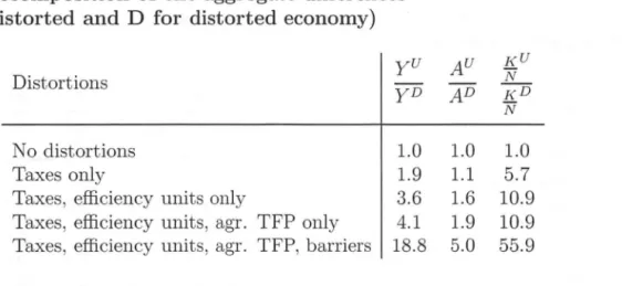
Table 4: Decomposition of the aggregate differences
(U for undistorted and D for distorted economy)
yU
Distortions yD
No distortions 1.0
Taxes only 1.9
Taxes, efficiency units only 3.6
Taxes, efficiency units, agr. TFP only 4.1
Taxes, efficiency units, agr. TFP, barriers 18.8
A U KU N AD KD N 1.0 1.0 1.1 5.7 1.6 10.9 1.9 10.9 5.0 55.9
Table 4 reports that barriers to entry account for 52 percent of the total income
difference.15 Higher taxes and lower efficiency units of labor account for 22 percent each
while lower agricultural TFP accounts only for 4 percent of the income gap with the
15Since the effects are multiplicative this fo11ows by taking logs:
10g(18.8) - 10g(4.1) = 0.52.
10g(18.8)
D.S. Interestingly our number for the effect of lower efficiency units in the poor country is dose to what development-accounting studies find for the effect of 1o-w endowment with human capital; see for example Hall and Jones (1999), Hendricks (2002), and ? This is remarkable because our calibration strategy does not use any information about cross-country differences in years of schooling, from which these studies construct their measures of human capital. The fact that our estimates nonetheless are broadly in line with their estimates lends support to the view that unmeasured quality differences in human capital may not be large.16
Table 4 also reports that barriers to entry account for most of the cross-country difference in aggregate TFP A. Moreover, barriers to entry together with low agricultural TFP account for almost the whole cross-country difference in aggregate TFP. This means that taxes must affect the aggregate economy mainly through reducing the capital-labor ratio. Indeed, the table shows that the cross-country difference in taxes account for a sizeable part of the cross-country difference iri the capital-labor ratio.
Table 5: Decomposition of the sectoral differences (U for undistorted and D for distorted economy)
..
!JJ
.
Y
yiUbY
&
Y
Distortions Na yD Ni Na Na yiD b D gD ~ ~ Na Ni Na Na No distortions 1.2 1.0 1.0 1.0 Taxes only 3.1 1.8 4.5 5.7Taxes, efficiency units only 5.6 3.4 8.7 10.9 Taxes, efficiency units, agr. TFP only 19.6 3.4 8.7 10.9 Taxes, efficiency units, agr. TFP, barriers 121.5 8.2 122.7 154.5
We did not target directly the cross-country differences in sectorallabor productivity.
Table 5 reports that they come out more than fifteen times larger in agriculture than in manufacturing. The prediction that there is a much larger labor-productivity gap in
agriculture is consistent with the evidence Restuccia et al. (2006) reporto Note that the 16Erosa et aI. (2005) and Manuelli and Seshadri (2005) have recently taken the opposite view.
.
.
,~
,
.
magnitudes of our findings are hard to relate to their's because their data set is from 1985 and it does not contain many of the 34 economies that make up our poor country. Note too that even if there are no distortions there remains a small labor productivity difference in agriculture. This comes from the fact that the poor country has a lower land
endowment than the USo
It is important to realize that cross-country difference in barriers to entry into nonagr
i-culture drive most of the uneven cross-country differences in sectoral labor productivity:
without barriers the gap with the U.S. in agriculture is about 6 times larger than in nonagriculture whereas with barriers it about 15 larger. There are two main reasons for
this. The first one is as in Restuccia et al. (2006): the fixed factor land implies that
returns to the reproducible production factors in agriculture are decreasing. So if in poor
countries a majority of the population farms to produce the leveI of food consumption dose to the subsistence leveI, then the land-labor ratio will be low in agriculture. The second reason why barriers to entry drive most of the uneven cross-country differences in sectoral labor productivity is that they drastically reduce the intermediates-labor and
capital-labor ratios in agriculture, as we discussed at the end of section 4.
6
Discussion
In this section we discuss our modeling choices. We also discuss the robustness of our results to alternative modeling choices.
6.1
Insider
groups choose TFP directly
We start with our assumption that each insider group chooses TFP directly and without any cost. This is a convenient reduced form that represents any choice or lobbying effort that reduce TFP. Real-world examples indu de the blocking of new and more productive
technologies and the stipulation of inefficient work practices or low effort. Concrete ex-amples for the latter are the number of holidays, staffing requirements, task descriptions,
the number of breaks, and monitoring procedures.17
Our specification is consistent with lower than possible TFP resulting from the use of inefficient technologies or from the inefficient use of a given technology. All that matters is that the frontier technology or the most efficient work rules and practices are available as public goods once the richest countries have innovated them.18 All other countries can then adopt them without having to innovate them again. The assumption that adoption
is costless simplifies matters but does not drive our result that insider groups choose lower than possible sector TFPs.
6.2
Monopoly power
only in
the labor market
Our rent-extraction mechanism is a special case. The general case would have monopoly power in both the goods and the labor market, so rents would go to both firmsjentrepre-neurs and workers. In terms of modeling, this would come at the costs of having several parameters, which would be messy and hard to discipline using the existing evidence.
Examples of the general case (and its problems) are Cole and Ohanian (2004) and Spector
(2004). Our special case has the monopoly power only in labor market, so rents go to workers only. This has the advantage of having just two parameters (the entry barriers
AO and the size of the insider group
À),
which is simple and can be calibrated. Examplesof our special case (and its advantages) are Holmes and Schmitz Jr. (1995) and Parente
and Prescott (1999). In sum, the reason for using our simple rent extraction mechanism is that it is parsimonious and analytically tractable while delivering that barriers to entry
lead to economic rents and low TFP.
17Clark (1987), Wolcott (1994), McKinsey-Global-Institute (1999), Rolmes and Schmitz (2001a,b), Parente and Prescott (2000), Galdon-Sanchez and Schmitz Jr. (2002), Lewis (2004), and Schmitz Jr.
(2005) ofIer real-world examples of how these are used.
18Romer (1990) provides a model of endogenous growth through innovations. Ris model may be thought of .,0; describing the technology leader who comes up with what the followers can adopt or block.
'
.
..
..
.
'
-,
'.
6.3
Insider groups cannot choose wages
or
hours worked
In om model the insider groups can choose TFP, but not wages or homs worked. We could incorporate a wage choice as in Parente and Prescott (1999) without changing any of om results. We leave it out because this would complicate om analysis fmther. In contrast, it is restrictive to assume that the insider groups cannot choose how much time the insiders work. If they could, then they could restrict their sectors' outputs by choosing low insider working time and high insider TFP. If leisure is a normal good, then this would
lead to higher insider utility than reducing sector TFP [Cozzi and Palacios (2003)]. We nonetheless abstract from the choice of homs worked because there is no evidence that hours worked in developing countries are systematically lower than in the OECD countries. If anything, the opposite seems to be true. Given the evidence that there are insider groups in developing countries, they do not seem to succeed at collectively reducing their members' homs worked by substantial amounts. Moreover, Clark (1987), Wolcott (1994), McKinsey-Global-Institute (1999), and Parente and Prescott (2000) pro-vide evidence that rent extraction in deveIoping countries happened through the choice of inefficient work ruIes and practices, and not through reductions in homs worked.
To be sure, in a few European countries insider groups succeeded at collectively reduc
-ing their members homs worked. In particular, Prescott (2004) documents that France has much lower homs worked and higher labor productivity than the V.S. This out-come requires a close cooperation between centralized labor unions and the government. Even in the V .S., trade unions have never reached a similar degree of centralization as in France. One should therefore expect that rent extraction in the V.S. has not
hap-pened through reductions in homs. Holmes and Schmitz (200la,b), Galdon-Sanchez and
Schmitz J1'. (2002), and Schmitz J1'. (2005) document various case studies where indeed rent extraction has instead happened through labor unions choosing inefficient work rules and practices. The rent extraction process in most developing countries seems too chaotic to replicate even V.S. outcomes, so it is not smprising that insider groups there do not seem to succeed at reducing the hours worked by their members.
6.4 Insider groups stay together forever
8ince we study steady-state equilibrium we fil' it natural to assume that the insider groups stay together forever. We emphasize that the duration of insider groups is not crucial for our results though. The reason is that each insider group's problem boils down to choosing the sector TFP that maximizes the insider wage in the next period; see appendix A.3.1. 80 one period is the minimum duration of insider groups required for our results. In what follows we suggest two alternative specifications in which the insider groups last exactly one period.
The first alternative would be to assume that in each period the members of the different insider groups are randomly chosen among alI the insiders. 8ince in symmetric steady state equilibrium alI insiders are identical, each insider group would still only need
to know the average capital holdings of its members to maximize their utility. Thus,
nothing would change.
The second alternative would be to assume that in each period the members of the insider groups are randomly chosen from the whole population. The individual capital holdings would then depend on how many times each individual has been chosen to be an insider in the past, so we would have a distribution of individual capital holdings. Besides
complicating the notation greatly (and being pretty unrealistic), this would not matter
for our results either. The first reason is that our preferences allow for aggregation, so the distribution of individual capital holdings would not have any effect on the aggregates of consumer choices. The second reason is that, as each insider group's problem boils down
to maximizing insider wage income, the distribution of capital holding would not matter.
6.5 Why don't societies buy the insider groups out?
Rent extraction through inefficient work rules and practices leads to substantial losses of income. This raises the question why the outsiders in our model do not buy out the insider groups. Our mo deI remains silent on how insider groups originate and disappear, so it cannot address buy outs. Taking the distortion as given without explaining its origin
is common practice in the part of the growth and development literature that explores
.' the implications of distortions. We view this as a useful first step in identifying the most
damaging distortions, given that they exist in the real world.
The next step is to understand how the distortions can emerge and why they can
persisto This requires an altogether different modeling approach that brings out political
economy forces at the cost of the quantitative richness of the model economy. In this
line of research, Krussel and Ríos-Rull (1996) and Bridgeman et aI. (2007) made some
progress on the question why barriers emerge. They formalized the argument of Olson
(1982) that if the costs of erecting barriers to entry to each industry are small, then they will be erected. In Krussel and Ríos-Rull (1996) this works through voting whereas in
Bridgeman et aI. (2007) this works through lobbying. Unfortunately, both of these mo deIs
are still far too stylized to be carried too the data.
We would also like to understand why society cannot buy out insider groups through
compensatory schemes. The literature offers two answers. Parente and Prescott (1999)
argued informally that compensatory schemes are not time consistent: once barriers to
entry have been removed, society can tax away the compensatory transfers it paid to
the groups or erect new barriers to entry. Kocherlakota (2001) showed in a stylized static model that limited enforcement and sufficient inequality can imply that a Pareto
-improving compensatory scheme does not existo More work is needed to formalize these
arguments in a dynamic setting that can be carried to the data.
References
Acemoglu, Daron, "The Form of Property Rights: Oligarchic vs. Democratic Societies,"
Manuscript, Massachusetts Institute of Technology 2005.
- - and FabrÍzio Zilibotti, "Productivity Differences," Quarterly Journal of
Eco-nomics, 2001, 115, 563-606.
- - and James A. Robinson, "Political Losers as a Barrier to Economic Deve lop-ment," American Economic Review (Papers and Proceedings), 2000, 90, 126-130.
Alesina, Alberto, Silvia Ardagna, Giuseppe Nicoletti, and Fabio Schiantarelli, "Regulation and Investment," Working Paper 9560, NBER 2003.
Amaral, Pedro and Erwan Quintin, "Finance Matters," NIanuscript, Federal Reserve Bank of Dallas and Southern Methodist University 2004.
Bridgeman, Benjamin R., Igor D. Livshits, and James C. MacGee, "Vested Interests and Technology Adoption," Journal of Monetary Economics, 2007, 54,
649-666.
Caselli, Francesco, "Accounting for Cross-Country Income Differences," in Philippe
Aghion and Steven Durlauf, eds., Handbook of Economic Growth, EIsevier, Forthcom
-ing: 2005, chapter 9.
- -and Wilbur John Coleman, "The U.S. Structural Transformation and Regional Convergence: A Reinterpretation," Journal of Political Economy, 2001, 109, 584-616. Clark, Gregory, "Why Isn't the Whole World Developed? Lessons from the Cotton
Mills," Journal of Economic History, 1987, 47, 141-173.
Cole, Harold L. and Lee E. Ohanian, "New Deal Policies and the Persistence of the Great Depression," Journal of Political Economy, 2004, 112, 779-816.
Cooley, Thomas F. and Edward C. Prescott, "Economic Growth and Business
Cycles," in Thomas F. Cooley, ed., Frontiers of Business Cycle Research, Princeton University Press, 1995.
Cozzi, Guido and Luis-Felipe Palacios, "Parente and Prescott's Theory May Work in Practice But Does Not Work in Theory," Contributions to Macroeconomics, E.E.
Journals, 2003, 3.