Heterogeneity and Aggregation
Richard Blundell and Thomas M. Stokery
November 2006
Abstract
This survey covers recent solutions to aggregation problems in three application areas, consumer demand analysis, consumption growth and wealth, and labor participation and wages. Each area involves treatment of heterogeneity and nonlinearity at the individual level. Three types of het-erogeneity are highlighted: hethet-erogeneity in individual tastes, hethet-erogeneity in income and wealth risks and heterogeneity in market participation. Work in each area is illustrated using results from empirical data. The overall aim is to show how concerns faced by empirical researchers regarding aggregation can be addressed.
Acknowledgements: A previous version of this chapter was published in theJournal of Economic Literature, vol. 43, 2, pp. 347-391, We are grateful for comments from numerous colleagues, especially Orazio Attanazio, Martin Browning, Jim Heckman, Arthur Lewbel and the reviewers. Thanks are also due to Howard Reed and Zoe Old…eld who helped organise the data for us. Financial support from the ESRC Centre for the Micro-Economic Analysis of Fiscal Policy at IFS is gratefully acknowledged. The usual disclaimer applies.
1. Introduction
Di¤erent people do, in fact, behave di¤erently. To describe the behavior of a group, one must
come to grips with this heterogeneity. In terms of empirical research in economics, this means facing
and resolving aggregation problems.
Aggregation problems are more than a cloying annoyance in empirical work. They exist at virtually
every level, from the initial issues of data construction and model speci…cation to the subsequent issues
Institute for Fiscal Studies and Department of Economics, University College London, Gower Street, London, WC1E 6BT.
y Sloan School of Management, Massachusetts Institute of Technology, 50 Memorial Drive, Cambridge, MA 02138
of how to usefully summarize and apply results. Because of their broad reach, aggregation problems
have traditionally been kept closeted within the practice of empirical work, along with other issues
for which there are no simple answers. But recently, this is changing, as there has been substantial
progress in dealing with aggregation problems in applied research. This survey covers much of this
development.
At the outset we must address a basic question: why consider aggregation problems at all? One
could take the view that economics is mainly about the behavior of individuals or of individual markets,
and assert a methodological position that only analysis of such individuals or individual markets makes
any real sense. However, such a view eliminates the applicability of the tenets of economic behavior to
some of the most important questions in economics, namely those that concern economic aggregates.
Economic policy is most often concerned with prices, interest rates, aggregate consumption and savings,
market demand and supply, total tax revenues, aggregate wages, unemployment, and so forth. The
valuation and allocation of scarce resources requires that attention be paid to large groups of individuals.
It is important to study relationships among economic aggregates, and to bring individual economic
behavior to bear on those relationships. Addressing aggregation problems just means creating a bridge
between those behaving individuals and the economic aggregates. After stating this goal, however, we
immediately meet several vexing issues as to how to even start to think about linking ‘individual’ and
‘aggregate.’
At one extreme are the almost philosophical issues of where, or at what level, to apply the strictures
of economic theory. Are we to assume that regularities associated with rationality apply to entire
economies, to ‘reasonably homogeneous’ groups of households, …rms or other types of economic agents,
or to Hicks’ Mr. Brown or Mr. Jones,1 as well as any of our own relatives or neighbors. To assert
that there is a ‘correct’ individual level at which to apply a mathematical model that is in line with
rational behavior is to take a stand on those issues; a stand which could only be properly validated by
experimentation or much more extensive empirical research than has been performed to date.2
1See Hicks(1956, p. 55).
2This e¤ort is underway, primarily in work on psychological tendencies in economics, …nance and marketing. This
At the other extreme are questions pertaining to what the appropriate ‘aggregate’ is. One typically
considers sums or averages as reported in national income accounts as the relevant aggregates. They
are usually the most interpretable numbers, and the most relevant for pricing or policy analysis. But
with large populations, one could consider many other kinds of aggregates, or statistics from the
population.3
Once these issues are settled – what is the relevant "individual level" and what is the relevant
"aggregate" – then aggregation problems become purely practical. For any application, a model must
be speci…ed which captures all important economic e¤ects, allows for relevant individual heterogeneity,
and bridges the gap between individual and aggregate, facilitating analysis at both levels.
This survey covers speci…c solutions and related work in primarily three application areas: consumer
demand analysis, consumption and saving analysis and analysis of wages and labor market
participa-tion. A key issue is to identify what kinds of individual di¤erences, or heterogeneity, are relevant for
each application area. As an organizing principle, we consider (i) heterogeneity in individual tastes
and incomes, (ii) heterogeneity in wealth and income risks faced by individuals and (iii) heterogeneity
in market participation.4 There is a generic tension between the degree of individual heterogeneity
accounted for and the ease with which one can draw implications for economic aggregates. We point
out how di¤erent types of heterogeneity are accommodated in the di¤erent application areas.
Our approach is practical, and we hope to address many of the concerns faced by empirical research
regarding aggregation. We take a “micro-econometric” view of the individual model – namely an
econometric model (obeying restrictions of economic theory) is applicable to individuals or households.
We consider model speci…cations that are typically used in empirical analysis of individual data, in
each application area. We take the relevant “aggregates” to be either totalled or per-capita (averaged)
values of the individual variables of interest, coinciding with aggregates as typically reported for regions
or whole economies. Whether such aggregates are easy to model or not, they are the most interpretable,
3For instance, to study inequality, a relevant aggregate would be the Gini coe¢cient. The choice of aggregate may
even be informed by empirical regularities in individual data. For example. if an individual model is best speci…ed with the logarithm of observed income, the geometric mean of income might be a more natural aggregate than total income or average income.
4This roughly coincides with the categorization of heterogeniety discussed in Browning, Hansen and Heckman (1999,
and the most useful types of aggregates for interpretation, policy analysis or other uses of empirical
results.
We are concerned with models that strike a balance between realism (‡exibility), adherence to
restrictions from economic theory and connections between individual behavior and aggregate statistics.
We consider several settings where individual models are intrinsically nonlinear, and for those we must
make speci…c assumptions on the distributions of relevant heterogeneous characteristics. We present
results that can be used to explore the impact of heterogeneity in empirical applications, that assume
reasonable (and hopefully plausible) parametrizations of both individual equations and distributions of
heterogeneity. We do not go into details about estimation; but for each application area we will present
models with empirically plausible equations for individuals, and consistent equations for the relevant
economic aggregates. The point is to have the ability to address empirical issues at the individual
(micro) level, the aggregate (macro) level, or both.
We begin with our coverage of consumer demand models in Section 2, the area which has seen
the most extensive development of solutions to aggregation problems. The di¢cult issues in consumer
demand include clear evidence of nonlinearity in income e¤ects (e.g. Engel’s Law for food) and pervasive
evidence of variations in demand with observable characteristics of households. We discuss each of these
problems in turn, and use the discussion to cover traditional results as well as ‘aggregation factors’ as
a method of empirically studying aggregation bias. We cover recent empirical demand models, and
present aggregation factors computed from data on British households. That is, we cover the standard
issues faced by aggregating over heterogeneous households in a static decision-making format, and
illustrate with application to empirical demand models in current use. We close with a discussion of
recent work that studies aggregate demand structure without making speci…c behavioral assumptions
on individual demands.
In Section 3 we discuss models of overall consumption growth and wealth. Here we must consider
heterogeneity in tastes, but we focus on the issues that arise from heterogeneity in income shocks,
showing how di¤erent types of shocks transmit to aggregate consumption. We start with a discussion
of quadratic preferences in order to focus on income and wealth, and then generalize to recent empirical
make explicit distributional assumptions to solve for aggregate equations. We cover the types of
heterogeneity found in consumption relationships, as well as various other aspects of our modeling,
illustrating with empirical data. We follow this with a brief discussion of modeling liquidity constraints
and the impacts on aggregate consumption. We close this section with a discussion of recent progress
in general equilibrium modeling of consumption, saving and wealth.
Section 4 covers recent work on labor participation and aggregate wage rates. The main issues
here concern how to interpret observed variations in aggregate wages – are they due to changes in
wages of individuals or to changes in the population of participating workers? We focus on the
issues of heterogeneity in market participation, and develop a paradigm that allows isolation of the
participation structure from the wage structure. This involves tracking the impacts of selection on
the composition of the working population, the impacts of weighting individual wage rates by hours
in the construction of aggregate wages, and the impact of observed wage heterogeneity. We show how
accounting for these features gives a substantively di¤erent picture of the wage situation in Britain
than that suggested by observed aggregate wage patterns. Here we have a situation where there is
substantial heterogeneity and substantial nonlinearity, and we show how to address these issues and
draw conclusions relevant to economic policy.
Section 5 concludes with some general observations on the status of work on aggregation in
eco-nomics.
This paper touches on many of the main ideas that arise in addressing aggregation problems, but
it is by no means a comprehensive survey of all relevant topics or recent approaches to such problems.
For instance, we limit our remarks on the basic nature of aggregation problems, or how it is senseless to
ascribe behavioral interpretations to estimated relationships among aggregate data without a detailed
treatment of the links between individual and aggregate levels. It is well known that convenient
constructs such as a ‘representative agent’ have, in fact, no general justi…cation, we will not further
belabor their lack of foundation. See the surveys by Stoker (1993) and Browning, Hansen and Heckman
(1998) for background on these basic problems. It is useful to mention two related lines of research,
that we do not cover. The …rst is the work on how economic theory provides few restrictions on market
others, and Donald J. Brown and Rosa L. Matzkin (1996) for a recent contribution. The second is the
work on collective decision making within households as pioneered by Pierre-Andre Chiappori (1988,
1994).
We will also limit our attention to aggregation over individuals, and not discuss the voluminous
literature on aggregation over commodities. This latter literature concerns the construction of
aggre-gate ‘goods’ from primary commodities, as well as the consistency of multistage budgeting and other
simpli…cations of choice processes. While very important for empirical work, the issues of commodity
aggregation apply within decision processes of individuals and, as such, would take us too far a…eld
of our main themes. See the survey by Blundell (1988) as well as the book Blackorby, Primont and
Russell (1978) for background on commodity aggregation and multistage budgeting. Moreover, we
do not cover the growing literature on hedonic/characteristics models, which can serve to facilitate
commodity aggregation or other simpli…cations in decision making.
Finally, we do not cover in great detail work that is associated with time series aggregation. That
work studies how the time series properties of aggregate statistics relate to the time series processes of
associated data series for individuals, such as stationarity, co-integration, etc. To permit such focus,
that work relies on strictly linear models for individual agents, which again, turn the discussion away
from heterogeneity in individual reactions and other behavior. We do make reference to time series
properties of income processes as relevant to our discussion of individual and aggregate consumption,
but do not focus on time series properties in any general way. Interested readers can pursue Granger
(1980, 1987, 1990) and the book by Forni and Lippi (1997) for more comprehensive treatment of this
literature.5
2. Consumer Demand Analysis
We begin with a discussion of aggregation and consumer demand analysis. Here the empirical
problem is to characterize budget allocation to several categories of commodities. The individual
level is that of a household, which is traditional in demand analysis. The economic aggregates to be
5See Stoker (1986c, 1993) and Lewbel (1994) and others for examples of clear problems in inferring behavioral reactions
modelled are average (economy-wide, per household) expenditures on the categories of commodities.
We are interested in aggregate demand, or how average category expenditures relate to prices and the
distribution of total budgets across the economy.
In a bit more detail, we assume that households have a two-stage planning process, where they set
the total budget for the current period using a forward looking plan, and then allocate that current
budget to the categories of non-durable commodities.6 As such, we are not concerned with
heterogene-ity in the risks faced by households in income and wealth levels – they have already been processed by
the household in their choice of total budget (and, possibly, in their stocks of durable goods). We
con-sider commodity categories that are su¢ciently broad that household expenditures are non-zero (food
categories, clothing categories, etc.), and so we are not concerned with zero responses, or heterogeneity
in market participation.
We are concerned with heterogeneity in total budgets and in needs and tastes. It is a
well-known empirical fact that category expenditure allocations vary nonlinearly with total budget size
(for instance, Engel’s Law with regard to food expenditures). Early applications of exact aggregation
demand systems had budget shares in semi-log form (with or without attributes), namely the popular
Translog models of Jorgenson, Lau and Stoker (1980, 1982) and Almost Ideal models of Deaton and
Muellbauer (1980a,b) respectively. More recent empirical studies have shown the need for further
nonlinear terms in certain expenditure share equations. In particular, evidence suggests that quadratic
logarithmic income terms are required (see, for example, Atkinson, Gomulka and Stern. (1990), Bierens
and Pott-Buter (1990), Hausman, Newey and Powell (1994), Härdle, Hildenbrand and Jerison (1991),
Lewbel (1991) and Blundell, Pashardes and Weber (1993)). This nonlinearity means that aggregate
demands will be a¤ected by total budget size as well as the degree of inequality in budgets across
consumers. It is also well known that category expenditures vary substantially with demographic
composition of households, such as how many children are present, or whether the head of household
is young or elderly, see Barten A.P. (1964), Pollak and Wales (1981), Ray (1983) and Browning (1992).
Our aim is to understand how behavioral e¤ects for households impinge on price e¤ects and
distrib-6Provided that intertemporal preferences are additive, this accords with a fairly general intertemporal model of expected
utional e¤ects on aggregate demands. Understanding these e¤ects is a key ingredient in understanding
how the composition of the population a¤ects demand growth over time and relative prices across the
di¤erent commodity categories.
2.1. Aggregation of Consumer Demand Relationships
Our framework requires accounting for individuals (households), goods and time periods. In each
period t, individual ichooses demands qijt (or equivalently, expenditurespjtqijt) for j= 1; :::; J goods
by maximizing preferences subject to an income constraint, wherei= 1; :::; nt. Pricespjt are assumed
to be constant across individuals at any point in time, with pt = (p1t; :::; pJ t) summarizing all prices.
Individuals have total expenditure budget mit =Pjpjtqijt, or income for short,7 and are described by a vector of household attributes zit, such as composition and demographic characteristics. The
general form for individual demands is written
qijt=gjt(pt;mit; zit) (1)
This model re‡ects heterogeneity in incomemitand individual attributeszit. Speci…c empirical models
involve the speci…cation of these elements,8 including a parametric formula for gjt.
Economy-wide average demands and average income are
P
iqijt
nt
; j= 1; :::; J and
P
imit
nt
(2)
We assume that the population of the economy is su¢ciently large to ignore sampling error, and
represent these averages as the associated population means
Et(qijt); j= 1; :::; J andEt(mit): (3)
Our general framework will utilize various other aggregates, such as statistics on the distribution of
7It is common parlance in the demand literature to refer to ‘total budget expenditure’ as ‘income,’ as we do here. In
the later section on consumption, we return to using ‘income’ more correctly , as current consumption expenditures plus savings.
8For most of our discussion,z
consumer characteristics zit.
2.1.1. Various Approaches: Exact Aggregation and Distributional Restrictions
We begin by discussing various approaches to aggregation in general terms. From (1), aggregate
demand is given formally as
Et(qijt) =
Z
gjt(pt;mit; zit)dFt(mit; zit): (4)
where Ft(mit; zit) is the cross-section distribution of income and attributes at time t. At the simplest level, approaches to aggregation seek a straightforward relationship between average demand, average
income and average attribute values
Et(qijt) =Gjt(pt; Et(mit); Et(zit)) (5)
Theexact aggregation approach is based on linearity restrictions on individual preferences/demands gijt that allow the relationship Gjt to be derived in a particularly simple way, such that knowledge of
Gjt is su¢cient to identify (the parameters of) the individual demand model. Take for example,
gjt(pt;mit; zit) =b0j(pt)mit+b1j(pt)mitlnmit+b2j(pt)mitzit (6)
where we supposezitis a single variable that haszit= 1for an elderly household andzit= 0otherwise.
Individual demand has a linear term in income, a nonlinear term in income, and the slope of the linear
term is di¤erent for elderly households. All of these slopes can vary with pt. Now, aggregate demand
is
Et(qijt) =b0j(pt)Et(mit) +b1j(pt)E(mitlnmit) +b2j(pt)E(mitzit); (7)
which depends on average incomeEt(mit) and two other statistics,E(mitlnmit) andE(mitzit). The coe¢cients are the same in the individual and aggregate models, which is the bridge through which
individual preference parameters manifest in aggregate demands (and can be recovered using aggregate
In order to judge the impact of aggregation on demand, it is convenient to useaggregation factors.9
Write aggregate demand as
Et(qijt) =b0j(pt)Et(mit) +b1j(pt) 1tE(mit) lnE(mit) +b2j(pt) 2tE(mit)E(zit); (8)
where
1t=
E(mitlnmit)
E(mit) lnE(mit)
and 2t=
E(mitzit)
E(mit)E(zit)
(9)
The factors 1tand 2tshow how the coe¢cients in (7) are adjusted if individual demand is evaluated
at average income and average attributes, as in (8). 1t re‡ects inequality in the income distribution
through the entropy term E(mitlnmit) and 2t re‡ects the distribution of income of the elderly, as
the ratio of the elderly’s share in aggregate income E(mitzit)=E(mit) to the percentage of elderly
E(zit) in the population. Aggregation factors are useful for two reasons. First, if they are stable, then
aggregate demand has similar structure to individual demand. Second, their average value indicates
how much bias is introduced in estimation using aggregate data alone.10
In contrast, the distributional approach considers restrictions on the heterogeneity distribution Ft(mit; zit). Suppose the density dFt(mit; zit) is assumed to be an explicit function ofEt(mit),E(zit)
and other parameters, such as variances and higher order moments. Then with a general
nonlin-ear speci…cation of individual demands gijt, we could solve (4) directly, expressing aggregate demand
Et(qijt)as a function of those distributional parameters. Here, recovery of individual demand
parame-ters from aggregate demand would be possible with su¢cient variation in the distribution Ft(mit; zit)
overt.11
While conceptually di¤erent from exact aggregation, the distributional approach should not be
thought of as a distinct alternative in empirical modeling. With distribution restrictions, formulating
a model via direct integration in (4) may be di¢cult in practice. As such, distributional restrictions
9The use of aggregation factors was …rst proposed by Blundell, Pashardes and Weber (1993) 1 0For instance, in (8),b
1j(pt)is the coe¢cient ofmitlnmit, whereas b1j(pt) 1t is the coe¢cient ofE(mit) lnE(mit). If 1t is stable, 1t = 0, then b1j(pt) 1t is proportional tob1j(pt). In this sense, the structure of aggregate demand matches that of individual demand, but the use of aggregate data alone would estimate the individual coe¢cient with a proportional bias of 0.
1 1Technically, what is necessary for recoverability is completeness of the class of income-attribute distributions; see
are often used together with exact aggregation restrictions, combining simplifying regularities of the
income-attribute distribution with linearity restrictions in individual demands.
One example is with mean-scaling, as discussed in Lewbel (1990), where the distribution of income
does not change relative shape but just scales up or down. Mean scaling can arise with a redistribution
mechanism where individual budgets are all scaled the same, as inmit=mit 1(Et(mit)=Et 1(mit 1)).
This structure allows distributional statistics such as those in (7) to be computed from mean income
only.
Another example arises from (distributional) exclusion restrictions. Certain attributes can be
excluded from aggregate demand if their distribution conditional on income is stable over time; if
dFt(mit; zit) =fz(zitjmit)dFt (mit) (10)
wherefz(zitjmit) does not vary witht, then from (4),
Et(qijt) =
Z
gjt(pt;mit; zit)fz(zitjmit)dFt (mit) =
Z
gjt(pt;mit)dFt(mit): (11)
That is, zit and its distributional statistics are excluded from the equation for aggregate demand.
Aggregate demand re‡ects heterogeneity only through variation in the income distribution – there
is not enough variation in the zit distribution over t to recover the individual e¤ects from aggregate
demand. We discuss various other examples of partial distribution restrictions below.
2.1.2. Demand and Budget Share Models
There has been a substantial amount of work on the precise structure of individual preferences and
demands consistent with exact aggregation. The most well-known result of this kind is in the extreme
case where the aggregate model simply relates average demandsEt(qijt) to the vector of relative prices
pt and average expenditure Et(mit). Gorman (1953) showed that this required preferences to be
quasi-homothetic; with individual demands linear inmit.
demands of the form.
qijt=a0j(pt) +b0j(pt)h0(mit) +:::+bM j(pt)hM(mit) (12)
with aggregate demands given as
Et(qijt) =a0j(pt) +b0j(pt)Et[h0(mit)] +:::+bM j(pt)Et[hM(mit)]: (13)
As above, provided there is su¢cient variation in the statistics Et[h1(mit)]; :::; Et[hM(mit)], the
coe¢cients a0j(pt); b0j(pt), .. , bM j(pt), and hence individual demands, can be fully recovered from
aggregate data.
Lau (1977, 1982) originally proposed the exact aggregation framework, and demonstrated that
demands of the form (12) were not only su¢cient but also necessary for exact aggregation, or
aggre-gation without distributional restrictions (c.f. Stoker (1993) and Jorgenson, Lau and Stoker (1982)).
Muellbauer (1975) studied a related problem, and established results for the special case of (12) with
only two income terms.12 They both showed several implications of applying integrability restrictions
to (12). If demands are zero at zero total expenditure, then a0j(pt) = 0. The budget constraint
implies that one can seth0(mit) =mit, without loss of generality. With homogeneity of degree zero in
prices and incomes, one can assert the forms of the remaining income terms, which include the entropy
form h1(mit) = mitlnmit and the power form h1(mit) = mit. This theory provides the background requirements for speci…c exact aggregation demand models, such as those we discuss below.13
The tradition in empirical demand analysis is to focus on relative allocations, and estimate equations
for budget shares. The exact aggregation form (12) is applied to budget shares for this purpose. In
particular, if we set a0j(pt) = 0 and h0(mit) =mit in (12), then budget shares wijt=pjtqijt=mit take
on a similar linear form. We have
wijt=
pjtqijt
mit
=b0j(pt) +b1j(pt)h1(mit) +:::+bM j(pt)hM(mit) (14)
1 2Muellbauer (1975) studied the conditions under which aggregate budget shares would depend only on a single
repre-sentative income value, which turned out to be analogous to the exact aggregation problem with only two expenditure terms.
whereb0j(pt); :::; bM j(pt) and h1(mit); :::; hM(mit) are rede…ned in the obvious way. If we denote
indi-vidual expenditure weights as it=mit=Et(mit);then aggregate budget shares are
Et(pjtqijt)
Et(mit)
Et( itwijt) (15)
= b0j(pt) +b1j(pt)Et( ith1(mit)) +:::+bM j(pt)Et( ithM(mit))
The same remarks on recoverability apply here: the individual budget share coe¢cientsb1j(pt); :::; bM j(pt)
can be identi…ed with aggregate data with su¢cient variation in the distributional termsEt( ith1(mit));
... ,Et( ithM(mit))over time. As above, aggregation factors can be used to gauge the di¤erence
be-tween aggregate shares and individual shares. We have
Et(pjtqijt)
Et(mit)
= Et( itwijt) (16)
= b0(pt) +b1(pt) 1th1(Et(mit)) +::+bM(pt) M thM(Et(mit))
where by construction
kt=
Et( ithk(mit))
hk(Et(mit))
; k= 1; :::; M (17)
are the aggregation factors. These factors give a compact representation of the distributional in‡uences
that cause the aggregate model, and the elasticities derived from it, to di¤er from the individual model.
The budget share form (14) accommodates exact aggregation through the separation of income
and price terms in its additive form. As before, when integrability restrictions are applied to (14),
the range of possible model speci…cations is strongly reduced. A particularly strong result is due to
Gorman (1981), who showed that homogeneity and symmetry restrictions imply that the rank of the
J x (M+ 1) matrix of coe¢cients[bmj(pt)] can be no greater than 3. Lau (1977), Lewbel (1991) and
2.1.3. Aggregation in Rank 2 and Rank 3 Models
Early exact aggregation models were of rank 2 (for a given value of attributeszit). With budget
share equations of the form14
wijt=b0j(pt) +b1j(pt)h1(mit); (18)
preferences can be speci…ed that give rise to either the log-form h1(mit) = lnmit and the power form
h1(mit) =mit. Typically the former is adopted and this produces Engel curves that are the same as
those that underlie the Almost Ideal model and the Translog model (without attributes).15 In this case
aggregate shares have the form
Et(pjtqijt)
Et(mit)
=Et( itwijt) =b0j(pt) +b1j(pt) 1tlnEt(mit) (19)
where the relevant aggregation factor is the following entropy measure for the mit distribution:
1t=
Et( itlnmit) lnEt(mit)
= Et(mitlnmit)
Et(mit) lnEt(mit)
: (20)
where we have recalled that it =mit=Et(mit). The deviation of 1t from unity describes the degree
of bias in recovering (individual) price and income elasticities from aggregate data alone.
Distribution restrictions can be used to facilitate computation of the aggregate statistics as well as
studying the aggregation factors. For instance, suppose income is lognormally distributed, withlnmit
distributed normally with mean mt and variance 2mt. The aggregation factor (20) can easily be seen
to be
1t= 1 +
1
2 mt= 2mt + 1
: (21)
To the extent that the log mean and variance are in stable proportion, 1t will be stable. If the log
mean is positive, then 1t>1, indicating positive bias from usinglnEt(mit).
Distribution restrictions can also facilitate the more modest goal of a stable relationship between
aggregate budget shares and aggregate total expenditure. For instance, suppose that the total
expen-1 4This is Muellbauer’s(1975) PIGL form.
1 5It is worthwhile to note that with the power form, estimation of with aggregate data would be complicated, because
diture distribution obeys
Et(mitlnmit) =c1Et(mit) +c2Et(mit) lnEt(mit) (22)
Then aggregate budget shares are
Et(pjtqijt)
Et(mit)
=b0j(pt) +b1j(pt) (c1+c2lnEt(mit)) (23)
so that a relationship of the form
Et(pjtqijt)
Et(mit)
=eb0j(pt) +eb1j(pt) lnEt(mit) (24)
would describe aggregate data well.
Here, integrability properties from individual demands can impart similar restrictions to the
aggre-gate relationship. Lewbel (1991) shows that if individual shares
wijt=b0j(pt) +b1j(pt) lnmit (25)
satisfy symmetry, additivity and homogeneity properties, then so will
wijt=b0j(pt) +b1j(pt)( + lnmit): (26)
The analogy of (23) and (26) makes clear that ifc2= 1, then the aggregate model will satisfy symmetry,
additivity and homogeneity. As such, some partial integrability restrictions may be applicable at the
aggregate level.16
As we discuss in section 2.2 below, rank 2 models of the form (18) fail on empirical grounds.
Evidence points to the need for more extensive income e¤ects (for given demographic attributes zit),
such as available from rank 3 exact aggregation speci…cations. In particular, rank 3 budget share
systems that include terms in (lnmit)2 (as well as individual attributes) seem to do a good job of
…tting the data, such as the QUAIDS system of Banks, Blundell and Lewbel (1997), described further
1 6It is tempting to consider the case ofc
in section 2.2 below. In these cases, corresponding to the quadratic term (lnmit)2; there will be an
additional aggregation factor to examine,
2t=
Et it(lnmit)2 (lnEt(mit))2
=
Et mit(lnmit)2
Et(mit) (lnEt(mit))2
: (27)
In analogy to (22), one can de…ne partial distributional restrictions so that aggregate shares are well
approximated as a quadratic function oflnEt(mit).
2.1.4. Heterogeneous Attributes
As we noted in our earlier discussion, the empirical analysis of individual level data has uncovered
substantial demographic e¤ects on demand. Here we reintroduce attributeszit into the equations, to
capture individual heterogeneity not related to income. Since zit varies across consumers, for exact
aggregation, zit must be incorporated in a similar fashion to total expendituremit. The budget share
form (14) is extended generally to
wijt=b0j(pt) +b1j(pt)h1(mit; zit) +:::+bM j(pt)hM(mit; zit) (28)
Restrictions from integrability theory must apply for each value of the characteristicszit. For instance,
Gorman’s rank theory implies that the share model can be rewritten with two terms that depend on
mit, but there is no immediate limit on the number of h terms that depend only on characteristics
zit.17
Budget share models that incorporate consumer characteristics in this fashion were …rst introduced
by Jorgenson, Lau and Stoker (1980, 1982). Aggregation factors arise for attribute terms, that
nec-essarily involve interactions between income and attributes. The simplest factors arise for terms that
depend only on characteristics, as inhj(mit; zit) =zit, namely
z t =
Et( itzit)
Et(zit)
= Et(mitzit)
Et(mit)Et(zit)
(29)
1 7A simple linear transformation will not in general be consistent with consumer optimization. Blundell, Browning and
This can be seen as the ratio of the income weighted mean ofzit to the unweighted mean ofzit: Ifzit is
an indicator; sayzit= 1for households with children andzit= 0 for households without children, then z
jt is the percentage of expenditure accounted for by households with children, Et(mitzit)=E(mit); divided the percentage of households with children,Et(zit).
More complicated factors terms arise with expenditure-characteristic e¤ects; for example, ifhj(mit; zit) =
zitlnmit then the relevant aggregation factor is
z
1t=
Et( itzitlnmit)
Et(zit) lnEt(mit)
= Et(mitzitlnmit)
Et(mit)Et(zit) lnEt(mit)
(30)
As before, in analogy to (22), one can derive partial distributional restrictions so that aggregate shares
are well approximated as a function of Et(mit) and Et(zit).
2.2. Empirical Evidence and the Speci…cation of Aggregate Demand Models
2.2.1. What do Individual Demands Look Like?
Demand behavior at the individual household level is nonlinear. As we have mentioned, it is not
realistic to assume that demands are linear in total expenditures and relative prices. To illustrate
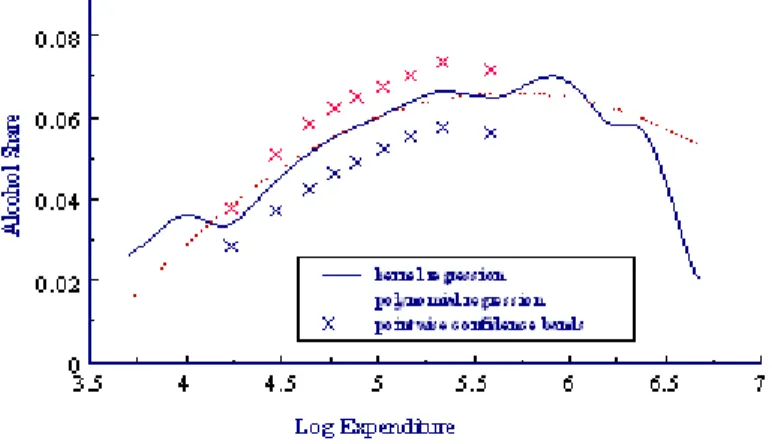
typical shapes of income structure of budget shares, Figures 1 and 2 present estimates of Engel curves
of two commodity groups for the demographic group of married couples without children, in the British
Family Expenditure Survey (FES).18 Each …gure plots the …tted values of a polynomial (quadratic)
regression in log total expenditure, together with a nonparametric kernel regression. We see that for
food expenditures, an equation that expressed the food share as a linear function of log expenditure
would be roughly correct. For alcohol expenditures, the income structure is more complex, requiring
quadratic terms in log expenditure. Moreover, as one varies the demographic group, the shapes of the
analogous Engel curves are similar, but they vary in level and slope.
The QUAIDS model of (Banks, Blundell and Lewbel (1997)) seems to be su¢ciently ‡exible to
1 8The FES is a random sample of around 7,000 households per year. The commodity groups are non-durable
Figure 1: Nonparametric Engel Curve: Food Share
capture these empirical patterns. In the QUAIDS model, expenditure shares have the form
wijt= j+ 0jlnpt+ j(lnmit lna(pt)) + j
(lnmit lna(pt))2
c(pt)
+uijt (31)
wherea(pt) and c(pt)are given as
ln a(pt) = 0
lnpt+ 12lnp 0 t lnpt; ln c(pt) =
0 lnpt;
with = ( 1; :::; N) 0
; = ( 1; :::; N)0; = ( 1; :::; N) 0 and = 0 B @ 0 1 .. . 0 N 1 C A:
This generalizes the (linear) Almost Ideal demand system by allowing nonzero i values, with the
denominator c(pt) required to maintain the integrability restrictions. Banks, Blundell and Lewbel
(1997) do extensive empirical analysis, and establish the importance of the quadratic log expenditure
terms for many commodities. Interestingly, they …nd no evidence of the rejection of integrability
restrictions associated with homogeneity or symmetry.
To include demographic attributes, an attractive speci…cation is the ‘shape invariant’ speci…cation
of Blundell, Duncan and Pendakur (1998). Suppose that gj0(lnmi) denotes a ‘base’ share equation,
then a shape invariant model speci…es budget shares as
wijt=gj0 lnmi (z 0
it ) +z 0 it'j:
The shape invariant version of the QUAIDS model allows demographic variation in the j terms. In
Banks, Blundell and Lewbel (1997), the j; j and j terms in (31) are allowed to vary with many
attributes zit.19 Family size, family composition, labor market status, occupation and education are
all found to be important attributes for many commodities.20
1 9For instance,
j+ 0jzitis used in place of j, and similar speci…cations for j and jterms.
2 0Various methods can be used to estimate the QUAIDS model, with the iterated moment estimator of Blundell and
2.2.2. The Implications for Aggregate Behavior
The stability and interpretation of aggregate relationships can be assessed from examining the
appropriate aggregation factors. We can compute the empirical counterparts to the factors by replacing
expectations with sample averages. For instance, 1t of (20) is estimated as
b1t=
P
i(bitlnmit)=nt ln(Pimit=nt)
(32)
and z
t of (29) is estimated as
^zt =
P
ibitzit=nt
P
izit=nt
(33)
where we recall that the weights have the form bit = mit=(Pimit=nt). Similarly, quadratic terms
in lnmit will require the analysis of the empirical counterpart to the term (27). Interactions of the
and terms with demographic attributes necessitates examination of the empirical counterparts of
terms of the form (30). We can also study aggregation factors computed over di¤erent subgroups of
the population, to see how aggregate demand would vary over those subgroups.
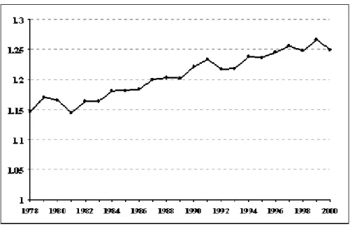
Figures 3 presents the estimated z
t term for the impact of children on household demands. This
shows a systematic rise in the share of non-durable expenditure and services attributable to families
with children over the 1980s and 1990s. The aggregate bias associated with using observed percentage
of households with children (as opposed to the income distribution across households with and without
children) varies from 15% to 25%. The path of z
t also follows the UK business cycle and the path of
aggregate expenditure with a downturns in 1981 and 1992.
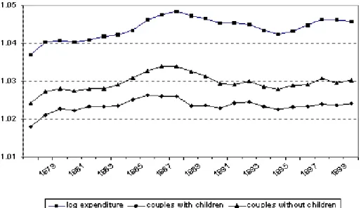
Figure 4 presents the estimated 1t and 2t terms relating to the lnmit and (lnmit)2 expressions
in the QUAIDS demand model. It is immediately clear that these also display systematic time series
variation, but in comparison to zt above, they increase over the …rst period of our sample and fall
towards the end. The bias in aggregation exhibited for the (lnmit)2 term is more than double that
exhibited for the lnmit term.
Figure 5 presents the aggregations factor forlnmitterm delineated by certain household types. The
baselinelnmline ("all") is the same as that in Figure 4. The other two lines correspond to interactions
Figure 3: Aggregation Factor for Households With Children
similar, they are at di¤erent levels, indicating di¤erent levels of bias associated with aggregation over
these subgroups.
Finally, it is worthwhile to mention some calculations we carried out on whether distributional
restrictions such as (22) are capable of representing the aggregate movements in total expenditure
data. Using the time series of distributional statistics from the FES data, we followed Lewbel (1991)
and implemented each of these approximations as a regression. With demographic interaction terms,
the aggregate model will only simplify if these conditions also apply to each demographic subgroup.
In virtually every case, we found the …t of the appropriate regressions to be quite close (sayR2 in the
range of .99). This gives support to the idea that aggregate demand relationships are reasonably stable
empirically. However, the evidence on the cjterms implies that aggregation factors are substantially
di¤erent than one, so again, estimates of the price and income elasticities using aggregate data alone
Figure 4: Aggregation Factors for Income Structure
2.3. Aggregation of Demand without Individual Structure
We close with discussion of a nontraditional approach given in Hildenbrand (1994), which is to
study speci…c aspects of aggregate demand structure without relying on assumptions on the behavior of
individual consumers. This work makes heavy use of empirical regularities in the observed distribution
of consumer expenditures across the population.
We can understand the nature of this approach from a simple example. Suppose we are interested
in whether aggregate demand for good j decreases when price pj increases (obeying the "Law of
Demand"), and we omit reference to other goods and time t for simplicity. Denote the conditional
expectation of demandqij for goodj, given incomemi and pricepj, as gj(pj;mi). Aggregate demand
for goodj is
E(qij) =G(pj) =
Z
g(pj;m)dF(m):
and our interest in in whether dG=dpj <0. Form this derivative, applying the Slutsky decomposition tog(pj; m) as
dG dpj
=
Z " dg
dpj comp g(pj;m) dg dm
#
dF(m) (34)
=
Z dg
dpj compdF(m)
Z
g(pj;m)
dg
dmdF(m)
= S A
The price e¤ect on aggregate demand decomposes into the mean compensated price e¤ect S and the
mean income e¤ect A. If we take S as negative, which is fairly uncontroversial, then we know that
dG=dpj <0if the income e¤ectA >0. Looking once more atAwe can see various ways of ascertaining
whether A >0 :
A=
Z
g(pj;m)
dg
dmdF(m) =
1 2
Z dhg(pj;m)2
i
dm dF(m) (35)
Without making any structural assumptions ong(pj; m), one could estimateAwith the …rst expression
This gives the ‡avor of this work without doing justice to the details. The main contribution
is to link up properties of aggregate demand directly with aspects of the distribution of demands
across the population. Hildenbrand (1998) shows that increasing spread is a common phenomena
in data on British households, and it is likely to be valid generally. More broadly, this work has
stimulated extensive study of the distribution of household expenditures, with a di¤erent perspective
than traditional demand modeling. Using nonparametric methods, Härdle, Hildenbrand and Jerison
(1991) study aggregate income e¤ects across a wide range of goods, and conclude that the ‘law of
demand’ likely holds quite generally. Hildenbrand and Kneip (1993) obtain similar …ndings on income
structure by directly examining the dimensionality of vectors of individual demands.21 See Hildenbrand
(1994) for an overview of this work, as well as Hildenbrand (1998) for an examination of variations in
the British expenditure distribution within a similar framework.
3. Consumption and Wealth
We now turn to a discussion of total consumption expenditures. Here the empirical problem is
to characterize consumption expenditures over time periods, including how they relate to income and
wealth. The individual level is typically that of a household (or an individual person, depending on
data source). The economic aggregate to be modeled is average consumption expenditures over time,
and we are interested in how aggregate consumption and saving relate to income and wealth across the
economy, as well as interest rates. This relationship is essential for understanding how interest rates
will evolve as the population changes demographically, for instance.
Consumption expenditures are determined through a forward looking plan, that takes into account
the needs of individuals over time, as well as uncertainty in wealth levels. There is substantial evidence
of demographic e¤ects and nonlinearities in consumption at the individual level,22 so we will need to
consider heterogeneity in tastes as before. Accordingly, aggregate consumption is a¤ected by the
structure of households and especially the age distribution, and aggregate consumption will be a¤ected
2 1This is related to transformation modeling structure of Grandmont (1992). It is clear that the dimensionality of
exact aggregation demand systems is given by the number of independent income/attribute terms, c.f. Diewert (1977) and Stoker (1984b).
by inequality in the distribution of wealth. We are not concerned here with heterogeneity in market
participation per se, as everyone has non-zero consumption expenditures. Later we discuss some
issues raised by liquidity constraints, which have much in common with market participation modeling
as described in Section 4.
Our primary focus is on heterogeneity with regard to risks in income and wealth levels, and how
the forward planning process is a¤ected by them. We take into account the nature of the income
and wealth shocks, as well as the nature of the credit markets that provide insurance against negative
shocks.
We consider four di¤erent types of shocks, delineated by whether the e¤ects are permanent or
transitory, and whether they are aggregate, a¤ecting all consumers, or individual in nature. Aggregate
permanent shocks can refer to permanent changes in the productive capability of the economy – such as
running out of a key natural resource, or skill-biased technical change – as well as to permanent changes
in taxes or other policies that a¤ect savings. Individual permanent shocks include permanent changes
in an individual’s ability to earn income, such as chronic bad health and long term changes in type and
status of employment. Aggregate transitory shocks refer to temporary aggregate phenomena, such as
exchange rate variation, bad weather, and so forth. Individual transitory shocks include to temporary
job lay-o¤s, temporary illnesses, etc. Many di¤erent situations of uncertainty can be accounted for by
combinations of these four di¤erent types of shocks.
In terms of risk exposure and markets, there are various scenarios to consider. With complete
markets, all risks are insured, and an individual’s consumption path is una¤ected by the evolution of
the individual’s income over time.23 When markets are not complete, the extent of available insurance
markets becomes important, and determines the degree to which di¤erent individual risks are
impor-tant for aggregate consumption behavior. For example, in the absence of credit market constraints,
idiosyncratic risks may be open to self-insurance. But in that case there may be little insurance
avail-able for aggregate shocks or even for permanent idiosyncratic shocks. Our discussion takes into account
the type of income risks and how risk exposure a¤ects aggregate consumption.
2 3See Atkeson and Ogaki (1996) for a model of aggregate expenditure allocation over time and to individual goods
Most of our discussion focuses on individual consumption plans and their implications for aggregate
consumption. Beyond this, we can consider the feedback e¤ects on consumption and wealth generated
through general equilibrium. For instance, if a certain group of consumers systematically save more
than others, then in equilibrium those consumers will be wealthier, and their savings behavior will be
a dominant in‡uence on the evolution of aggregate wealth. The study of this important topic is in its
infancy, and has been analyzed primarily with calibrated macroeconomic growth models. We include
a discussion of some of this work.
3.1. Consumption Growth and Income Shocks
In our framework, in each period t, individual i chooses consumption expenditures cit by maxi-mizing expected utility subject to an asset accumulation constraint. Individual i has heterogeneous
attributeszit that a¤ect preferences. There is a common, riskless interest rate rt. We assume
separa-bility between consumption and labor supply in each time period, and separasepara-bility of preferences over
time.
We begin with a discussion of aggregation with quadratic preferences. This allows us to focus on
the issues of di¤erent types of income shocks and insurance, without dealing with nonlinearity. In
Section 3.2, we consider more realistic preferences that allow precautionary saving.
When individual within-period utilities are quadratic in current consumption, we have the familiar
certainty-equivalent formulation in which there is no precautionary saving. Within-period utilities are
given as
Uit(cit) = 1
2(ait cit)
2 (36)
forcit< ait. We model individual heterogeneity by connectingait to individual attributes as
ait= + 0
zit (37)
With the discount rate equal to the real interest rate, maximizing the expected sum of discounted
utilities gives the following optimal plan for the consumer (Hall (1978)),
cit= it+ it = 0
De…ning i;t 1 as the information set for individualiin period t 1;the consumption innovation it
obeys
E[ itj i;t 1] = 0: (39)
In what follows we will use a time superscript to denote this conditional expectation, namelyEt 1( )
E[j i;t 1]to distinguish it from the population average in periodt(which uses a time subscript as in
Et( ) ): Notice, the model (38) is linear in the change in attributes zit with constant coe¢cients , plus the consumption innovation. In other words, this model is in exact aggregation form with regard
to the attributes zit that a¤ect preferences.
3.1.1. Idiosyncratic Income Variation and Aggregate Shocks
When the only uncertainty arises from real income, the consumption innovation itcan be directly
related to the stochastic process for income. We begin by spelling out the income process in a meaningful
way. Express incomeyit as the sum of transitory and permanent components
yit=yitP +yitT: (40)
and assume that the transitory component is serially independent. We assume that the permanent
component follows a random walk
yitP =yitP 1+ Pit (41)
where the innovation P
it is serially independent.
Next, decompose these two components into a common aggregate e¤ect and an idiosyncratic e¤ect
P
it = t+"it; (42)
yitT =ut+vit: (43)
Here t is the common aggregate permanent shock,"it is the permanent shock at the individual level,
utis the aggregate transitory shock andvitis the individual transitory shock – the four types of income
shocks discussed above. This mixture of permanent and transitory shocks has been found to provide
Pistaferri (2004). We assume that the individual shocks are normalized to average to zero across the
population, namely Et("it) = 0 and Et(vit) = 0.
The stochastic process for individual income then takes the form
yit= t+"it+ ut+ vit: (44)
The stochastic process for aggregate income has the form
Et(yit) = t+ ut (45)
where, again,Etto denotes expectation (associated with averaging) across the population of agents at timet:
3.1.2. Income Shocks and Insurance
The …rst scenario is where individual (and aggregate) shocks are not insurable. Here the optimal
consumption innovation it for the individual will adjust fully to permanent income shocks but only
adjust to the annuity value of transitory shocks. To see this, again suppose that real interest rates are
constant and equal the discount rate. Under quadratic preferences (36), consumption growth can be
written (Deaton and Paxson (1994))
cit= 0
zit+ t+"it+ t( ut+ vit); (46)
where tis the annuitization rate for a transitory shock with planning over a …nite horizon.24 Clearly,
expected growth is determined by preference attributes as
Et 1( cit) =E( citj i;t 1) = zit: (47)
Aggregate consumption has the form
Et(cit) = 0 Et(zit) + t+ t ut (48)
2 4IfL is the time horizon, then
t =r .h
(1 +r) (1 (1 +r) (L t+1))i . Clearly
Thus, the aggregate data is described exactly by a representative agent model with quadratic preferences
and characteristics Et(zit) facing a permanent/transitory income process.25
For the second scenario, suppose individual shocks can be fully insured, either through informal
processes or through credit markets. Now individual consumption growth depends only on aggregate
shocks
cit= 0
zit+ t+ t ut: (49)
Consequently, with (48), we will have
cit = 0
( zit Et(zit)) + Et(cit): (50)
Thus, consumption growth at the individual level equals aggregate consumption growth plus an
ad-justment for individual preferences.
Finally, the third scenario is where all shocks (aggregate and individual) are fully insurable. Now
individual consumption growth will be the planned changes 0 zit only, and aggregate consumption
growth will be the mean of those changes 0 Et(zit). This is the most complete "representative
agent" case, as complete insurance has removed the relevance of all income risks.
3.1.3. Incomplete Information
It is interesting to note that in our simplest framework, incomplete information can cause aggregate
consumption to fail to have random walk structure. In particular, suppose individual shocks are not
completely insurable and consumers cannot distinguish between individual and aggregate shocks. To
keep it simple, also assume that there are no varying preference attributes zit. Following Pischke
(1995), individualiwill view the income process (44) as an MA(1) process:
yit= it it 1; (51)
where the parameter is a function of the relative variances of the shocks.
2 5Aside from the drift term 0 E
t(zit), aggregate consumption is a random walk. In particular, the orthogonality conditions Et 1(
Changes in individual consumption are simply
cit= (1 ) it
Note that it is still the case that Et 1( c
it) =E( citj i;t 1) = 0. However, from (51) we have that
cit cit 1 = (1 ) yit (52)
Replacing yit by (44) and averaging over consumers we …nd
Et(cit) = Et 1(cit 1) + (1 )( t+ ut) (53)
so that aggregate consumption is clearly not a random walk.
3.2. Aggregate Consumption Growth with Precautionary Saving
With quadratic preferences, consumption growth can be written as linear in individual attributes –
in exact aggregation form – and we were able to isolate the impacts of di¤erent kinds of income shocks
and insurance scenarios. To allow for precautionary saving, we must also account for nonlinearity in
the basic consumption process. For this, we now consider the most standard consumption model used
in empirical work, that based on Constant Relative Risk Aversion (CRRA) preferences.
3.2.1. Consumption Growth with CRRA Preferences
We assume that within-period utility is
Uit(cit) =eait
2 4c
1 1
sit it 1 sit1
3
5 (54)
whereait permits scaling in marginal utility levels (or individual subjective discount rates), and sit is
the intertemporal elasticity of substitution, re‡ecting the willingness of individualito trade o¤ today’s
consumption for future consumption. As before, we will model the heterogeneity in ait and sit via
individual attributeszit.
log-form as
lnyit = t+"it+ ut+ vit: (55)
The permanent and transitory error components in the income process are decomposed into aggregate
and individual terms, as in (44). As noted before, this income growth speci…cation is closely in accord
with the typical panel data models of income or earnings, and it will neatly complement our equations
for consumption growth with CRRA preferences. In addition, we assume that the interest rate rt is small, for simplicity, and is not subject to unanticipated shocks.
With precautionary savings, consumption growth depends on the conditional variances of the
unin-surable components of shocks to income. Speci…cally, with CRRA preferences (54) and log income
process (55), we have the following log-linear approximation for consumption growth26
lncit= rt+ ( +'rt)0zit+k1 tit 1+k2 t 1
At + 1"it+ 2 t (56)
where tit1is the conditional variance of idiosyncratic risk (conditional ont 1information i;t 1) and
t 1
At is the conditional variance of aggregate risk. The attributes zit represent the impact of hetero-geneity in ait, or individual subjective discount rates, and the intertemporal elasticity of substitution
sit= + +'0zit. Typically in empirical applications,zitwill include levels and changes in observable attributes, and unobserved factors may also be appropriate.27 As before,
E("itj i;t 1) = Et 1("it) = 0 (57)
E( tj i;t 1) = Et 1( t) = 0 (58)
To sum up, in contrast to the quadratic preference case, the growth equation (56) is nonlinear in
consumption, and it includes conditional variance terms which capture the importance of precautionary
saving.
A consistent aggregate of the individual model (56) is given by
Et( lncit) = rt+ ( +'rt) 0
Et(zit) +k1Et( tit 1) +k2 t 1
At + 2 t (59)
2 6See Blundell and Stoker (1999) for a precise derivation and discussion of this approximation.
whereEt( lncit)refers to the population mean of the cross-section distribution of lncitin period t;
and so on. Thetsubscript again refers to averaging across the population of consumers, and we have
normalized Et("it) = 0as before. Provided Et(lncit 1) =Et 1(lncit 1), equation (59) gives a model
of changes over time in Et(lncit), which is a natural aggregate given the log form of the model (56).
However, Et(lncit) is not the aggregate typically observed nor is it of much policy interest. Of
central interest is per-capita consumptionEt(cit)or total consumptionntEt(cit). Deriving an equation
for the appropriate aggregates involves dealing with the ‘log’ nonlinearity, to which we now turn.28
3.2.2. How is Consumption Distributed?
Since the individual consumption growth equations are nonlinear, we must make distributional
assumptions to be able to formulate an equation for aggregate consumption. In the following, we will
assume lognormality of various elements of the consumption process. Here we point out that this
is motivated by an important empirical regularity – namely, individual consumption does appear to
be lognormally distributed, at least in developed countries such as the United States and the United
Kingdom.
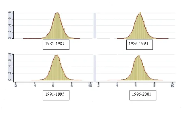
Figure 6 shows the distribution of log-consumption using US consumer expenditure data across
the last two decades. Consumption is taken as real expenditure on non-durables and services, and is
plotted by …ve year bands to achieve a reasonable sample size. Each log-consumption distribution
has a striking resemblance to a normal density. In the experience of the authors, this result is often
replicated in more disaggregated data by year and various demographic categorizations, such as birth
cohort, and also in other countries including in the Family Expenditure Survey data for the UK. Given
this regularity, one would certainly start with log-normality assumptions such as those we make below,
and any subsequent re…nements would need to preserve normality of the marginal distribution of log
consumption.
2 8If we evaluate the individual model at aggregate values, we get
lnEt(cit) = rt+ ( +'rt)Et(zit) +k2 tAt1+!t:
Here!t is a ‘catch-all’ term containing the features that induce aggregation bias, that will not satisfy the orthogonality conditionEt 1(!
3.2.3. Insurance and Aggregation with Precautionary Saving
As with our previous discussion, we must consider aggregation under di¤erent scenarios of
in-surance for income risks. We again assume that agents have the same information set, namely
i;t 1 = t 1 for all i; t.
We begin with the scenario in which there is full insurance for individual risks, or pooling of
idiosyncratic risk across individuals. Here insurance and credit markets are su¢ciently complete to
remove individual risk terms in individual income and consumption streams, so "it = 0 and tit1 = 0
for all i; t. The individual model (56) becomes
lncit= rt+ ( +'rt) 0
zit+k2 tAt1+ 2 t (60)
withEt 1(
t) = 0. The mean-log model (59) is now written as
Et(lncit) Et(lncit 1) = rt+ ( +'rt) 0
Et(zit) +k2 tAt1+ 2 t: (61)
The relevant aggregate is per-capita consumption Et(cit). Per-capita consumption is given by
Et(cit) = Et
h
exp lncit 1+ rt+ ( +'rt) 0
zit+k2 tAt1+ 2 t
i
(62)
= exp rt+k2 tAt1+ 2 t Et
h
cit 1exp ( +'rt) 0
zit
i
with the impact of log-linearity arising in the …nal term, a weighted average of attribute terms interacted
with lagged consumption cit 1.
Of primary interest is aggregate consumption growth, or the log-…rst di¤erence in aggregate
con-sumption
lnEt(cit) = ln
Et(cit)
Et 1(cit 1)
:
This is expressed as
lnEt(cit) = rt+k2 tAt1+ 2 t
+ ln Et
h
cit 1exp ( +'rt)
0 zit
i
Et(cit 1)
!
+ ln Et(cit 1) Et 1(cit 1) :
Aggregate consumption growth re‡ects the interest and risk terms that are common to all consumers,
a weighted average of attribute terms, and the log-di¤erence in the average of cit 1 at time t versus
timet 1.
Notice …rst that even if zit is normally distributed, we cannot conclude that lncit is normal. We
also need (as a su¢cient condition) thatlncit 1 is normal at timetto make such a claim. This would
further seem to require normality oflncit 2 att 1, and so forth into the distant past. In any case,
we cover this situation with the broad assumption:
The distribution of cit 1 is the same in period t 1and t: (64)
That is, the population could grow or shrink, but the distribution of cit 1 is unchanged. Under that
assumption, we can drop the last term in (63)
ln Et(cit 1)
Et 1(cit 1)
= 0: (65)
Lagging the individual model (60) gives an equation for cit 1, but there is no natural way to
incorporate that structure directly into the equation for aggregate current consumption Et(cit).29
Therefore, we further assume
lncit 1
0 tzit
~ N c 1t
0
tEt(zit)
;
" 2
c 1;t
0 zc 1;t t
0 t zc 1;t
0 t zz;t t
#!
: (66)
where we have set t= ( +'rt). This assumption says that
lncit 1+
0
tzit (67)
~N c 1t+
0
tEt(zit); 2c 1;t+
0
t zz;t t+ 2 0 t zc 1;t
and
lncit 1 ~ N c 1t;
2
c 1;t : (68)
2 9This is because of the potential dependence ofc
We can now solve for an explicit solution to (63): apply (65), (67) and (68) and rearrange to get
lnEt(cit) = rt+ ( +'rt)0Et(zit) +k2 tAt1+ 2 t
+12h( +'rt) 0
zz;t( +'rt) + 2 ( +'rt) zc 1;t
i (69)
This is the aggregate model of interest, expressing growth in per-capita consumption as a function of
the mean ofz, the conditional variance terms from income risk, and the covariances between attributes
z and lagged consumption cit 1. Thus shows how individual heterogeneity manifests itself in
aggre-gate consumption through distributional variance terms. These variance terms vary with rt if the
intertemporal elasticity of substitution varies over the population.
Now consider the scenario where some individual risks are uninsurable. This reintroduces terms "it
and tit 1 in consumption growth at the individual model, and we must be concerned with how those
permanent risks are distributed across the population. In particular, we assume in each period that
each individual draws idiosyncratic risk from a common conditional distribution, so that tit1 = tIt1
for all i. The individual consumption growth equation (56) now appears as
lncit= rt+ ( +'rt) 0
zit+k1 tIt1+k2 t 1
At + 1"it+ 2 t: (70)
The mechanics for aggregation within this formulation are similar to the previous case, including
the normalizationEt("it) = 0, but we need deal explicitly with how the permanent individual shocks
"it covary with ln cit 1. As above, we adopt a stability assumption (64). We then extend (66) to
assume that lncit 1;( +'rt) 0
zit; "it is joint normally distributed. The growth in aggregate average
consumption is now given by
lnEt(cit) = rt+ ( +'rt) 0
Et(zit) +k1 tIt1+k2 t 1
At + 2 t+ 1
2( t) (71)
where
t= ( +'rt) 0
zz;t( +'rt) + 21 2";t+ 2 ( +'rt) 0
zc 1;t
+2 1 "c 1;t+ 2 1 "z;t( +'rt):
While complex, this formulation underlines the importance of the distribution of risk across the
changing variance in consumption growth. The term tIt1captures how idiosyncratic risk varies, based
on t 1information.
We have not explicitly considered unanticipated shocks to the interest rate rt, or heterogeneity in
rates across individuals.30 Unanticipated shocks in interest would manifest as a correlation betweenr
t
and aggregate income shocks, and would need treatment via instruments in estimation. Heterogeneity
in rates could, in principle, be accommodated as with heterogeneous attributes. This would be
especially complicated if the overall distributional structure were to shift as interest rates increased or
decreased.
3.3. Empirical Evidence on Aggregating the Consumption Growth Relationship
There are two related aspects of empirical research that are relevant for our analysis of aggregation in
consumption growth models. The …rst concerns the evidence on full insurance of individual risks. How
good an approximation would such an assumption be? To settle this we need to examine whether there
is evidence of risk pooling across di¤erent individuals and di¤erent groups in the economy. For example,
does an unexpected change in pension rights, speci…c to one cohort or generation, get smoothed by
transfers across generations? Are idiosyncratic health risks to income fully insured? Even though we
may be able to cite individual cases where this perfect insurance paradigm clearly fails, is it nonetheless
a reasonable approximation when studying the time series of aggregate consumption?
The second aspect of empirical evidence concerns the factors in the aggregate model (71) that
are typically omitted in studies of aggregate consumption. From the point of view of estimating the
intertemporal elasticity parameter ;how important are these aggregation factors? How well do they
correlate with typically chosen instruments and how likely are they to contaminate tests of excess
sensitivity performed with aggregate data?
3.3.1. Evidence on Full Insurance and Risk Pooling Across Consumers
If the full insurance paradigm is a good approximation to reality, then aggregation is considerably
simpli…ed and aggregate relationships satisfying the standard optimality conditions can be derived
3 0Zeldes (1989b) points out how di¤ering marginal tax rates can cause interestr