www.ache.org.rs/CICEQ
Chemical Industry & Chemical Engineering Quarterly 14 (3) 191−203 (2008) CI&CEQ
S. K. LAHIRI K. C. GHANTA
Department of Chemical Engineering, NIT, Durgapur, West Bengal, India
SCIENTIFIC PAPER
UDC 537.314:621.3.012.1:621.315.2
THE SUPPORT VECTOR REGRESSION WITH
THE PARAMETER TUNING ASSISTED BY A
DIFFERENTIAL EVOLUTION TECHNIQUE:
STUDY OF THE CRITICAL VELOCITY OF
A SLURRY FLOW IN A PIPELINE
This paper describes a robust Support Vector regression (SVR) methodology, which can offer a superior performance for important process engineering pro-blems. The method incorporates hybrid support vector regression and a diffe-rential evolution technique (SVR-DE) for the efficient tuning of SVR meta para-meters. The algorithm has been applied for the prediction of critical velocity of the solid-liquid slurry flow. A comparison with selected correlations in the lite-rature showed that the developed SVR correlation noticeably improved the prediction of critical velocity over a wide range of operating conditions, physical properties, and pipe diameters.
Key words: support vector regression; differential evolution; slurry criti-cal velocity.
Conventionally, two approaches, namely
phe-nomenological (first principles) and empirical, are
em-ployed for the slurry flow modeling. The advantages of a phenomenological model are: (i) it represents a physico-chemical phenomenon underlying the pro-cess explicitly and (ii) it possesses the extrapolation ability. Owing to the complex nature of many multi-phase multi-phase slurry processes, the underlying physic-co-chemical phenolmenon is seldom fully understood. Also, the collection of the requisite phenolme-nological information is costly, time-consuming and tedious and therefore the development and the solu-tion of the phenomenological process models have considerable practical difficulties. These difficulties necessitate the exploration of the alternative modeling formalisms.
In the last decade, the artificial neural networks
(ANNs) and more recently, the support vector
regres-sion (SVR) have emerged as two attracttive tools for
non-linear modeling, especially in situations where the development of phenomenological or conventio-nal regression models becomes impractical or cum-bersome. In recent years, the support vector
Corresponding author: S. K. Lahiri, Department of Chemical En-gineering, NIT, Durgapur, West Bengal, India.
E-mail: [email protected] Paper received: May 7, 2008. Paper revised: August 29, 2008. Paper accepted: September 8, 2008.
sion (SVR) [1-3] which is a statistical learning theory based machine learning formalism is gaining popu-larity over ANN due to its numerous attractive fea-tures and a promising empirical performance.
The main difference between conventional ANNs and SVM lies in the risk minimization principle. The conventional ANNs implement the empirical risk mini-mization (ERM) principle to minimize the error on the training data, while SVM adheres to the Structural Risk Minimization (SRM) principle seeking to set up an upper bound of the generalization error [1-3].
This study is motivated by a growing popularity of the support vector machines (SVM) for regression problems. Although the foundation of the SVR para-digm was laid down in the mid 1990s, its chemical engineering applications such as fault detection [4,5] have emerged only recently.
Conventionally, various deterministic gradient based methods [6] are used for optimizing a process model. Most of these methods however require that the objective function should be smooth, continuous, and differentiable. The SVR models can not be gua-ranteed to be smooth, especially in regions wherein the input-output data (training set) used in model building is located sparsely. In such situations, an ef-ficient optimization formalism known as Differential Evolution (DE), which is lenient towards the form of the objective function, can be used. In the recent years, DEs that are members of the stochastic opti-mization formalisms have been used with a great suc-cess in solving problems involving very large search spaces. The DEs were originally developed as the ge-netic engineering models mimicking population evolu-tion in natural systems. Specifically, DE like a genetic algorithm (GA) enforces the “survival-of-the-fittest” and “genetic propagation of characteristics” principles of the biological evolution for searching the solution space of an optimization problem. DE has been used to design several complex digital filters [7] and to de-sign fuzzy logic controllers [8]. DE can also be used for parameter estimations, e.g. Babu and Sastry [9] used DE for the estimation of the effective heat trans-fer parameters in trickle-bed reactors using radial temperature profile measurements. They concluded that DE takes less computational time to converge, compared to the existing techniques, without compro-mising with the accuracy of the parameter estimates.
In the present paper, SVR formalism is integra-ted with the differential evolution to arrive at modeling and optimization strategies. The strategy (henceforth referred to as “SVR-DE”) use an SVR as the non-li-near process modeling paradigm, and the DE for opti-mizing the meta-parameters of the SVR model so that an improved prediction performance is realized. To our knowledge, the hybrid involving SVR and DE is being used for the first time for the chemical process modeling and optimization. In the present work, we propose a hybrid support vector regression-differen-tial evolution (SVR-DE) approach for tuning the SVR meta parameters and illustrate it by applying it for pre-dicting the critical velocity of the solid liquid flow.
SUPPORT VECTOR REGRESSION (SVR) MODELING
Support vector regression (SVR) is an adapta-tion of a recent statistical learning theory based clas-sification paradigm, namely “support vector machi-nes” [3]. The SVR formulation follows structural risk minimization (SRM) principle, as opposed to the empirical risk minimization (ERM) approach which is
commonly employed within statistical machine learn-ing methods and also in trainlearn-ing ANNs. In SRM, an upper bound on the generalization error is minimized as opposed to the ERM, which minimizes the predict-tion error on the training data. This equips the SVR with a greater potential to generalize the input-output relationship learnt during its training phase for making good predictions for new input data. The SVR is a linear method in a high dimensional feature space, which is nonlinearly related to the input space. Though the linear algorithm works in the high dimensional fea-ture space, in practice it does not involve any compu-tations in that space due to the usage of kernels; all necessary computations are performed directly in the input space. In the following, the basic concepts of SVR are introduced. A more detailed description of SVR can be found elsewhere [1,10-12].
Support vector regression: at a glance
Consider a training data set g = {(x1,y1),
(x2,y2),…,(xP,yP)}, such that xi∈ υN is a vector of input
variables and yi∈ υis the corresponding scalar
out-put (target) value. Here, the modeling objective is to find a regression function, y = f(x), such that it accura-tely predicts the outputs {y} corresponding to a new set of input-output examples, {(x,y)}, which are drawn from the same underlying joint probability distribution,
P(x,y), as the training set. To fulfill the stated goal, SVR considers the following linear estimation function:
f(x) = 〈w,φ(x)〉 + b (1)
where w denotes the weight vector; b refers to a con-stant known as “bias”; f(x) denotes a function termed
feature, and 〈w,φ(x)〉 represents the dot product in the
feature space, l, such φ: x→l, w ∈l. In SVR, the in-put data vector, x, is mapped into a high dimensional feature space, l, via a nonlinear mapping function, φ,
and a linear regression is performed in this space for predicting y. Thus, the problem of non-linear regres-sion in lower dimenregres-sional input space υN
is transfor-med into a linear regression in the high dimensional feature space, l. Accordingly, the original optimiza-tion problem involving non-linear regression is trans-formed into finding the flattest function in the feature space l and not in the input space, x. The unknown parameters w and b in Eq. (1) are estimated using the training set, g. To avoid over-fitting and thereby im-proving the generalization capability, the following re-gularized functional involving summation of the empi-rical risk and a complexity term w2
is minimized:
∑
=+ − =
+ =
P
i
i
i y w
x f C w
f R f R
1
2 2
emp
where Rreg and Rempdenote the regression and
empi-rical risks, respectively; w2
is the Euclidean norm; C is a cost function measuring the empirical risk, and λ>0 is a regularization constant. For a given function, f, the regression risk (test set error), Rreg[f], is the
pos-sible error committed by the function f in predicting the output corresponding to a new (test) example in-put vector drawn randomly from the same sample probability distribution, P(x,y), as the training set. The empirical risk, Remp[f], represents the error (termed
“training set error”) committed in predicting the out-puts of the training set inout-puts. The minimization task described in Eq. (2) involves: (i) the minimization of the empirical loss function Remp[f] and (ii) obtaining as
small a w as possible, using the training set g. The commonly used loss function is the “e-insensitive loss function” given as [2]:
ε − − =
−y f x y
x f
C( ( ) ) ( ) , for |f(x)−y|≥ε,
otherwise: C = 0 (3)
where ε is a precision parameter representing the ra-dius of the tube located around the regression func-tion (see Figure 1); the region enclosed by the tube is known as “e-intensive zone”. The SVR algorithm at-tempts to position the tube around the data as shown in Figure 1.
The optimization criterion in Eq. (3) penalizes those data points whose y values lie more than ε dis-tance away from the fitted function, f(x). In Figure 1, the size of the stated excess positive and negative deviations are depicted by ζ and ζ*, which are termed “slack” variables. Outside of the (-ε,ε) region, the slack variables assume non-zero values. The SVR fits f(x) to the data in a manner so that: (i) the training error is minimized by minimizing ζ and ζ* and (ii) w2
is
mini-mized to increase the flatness of f(x) or to penalize over the complexity of the fitting function. Vapnik [2] showed that the following function possessing the fi-nite number of parameters can minimize the regula-rized function in Eq. (2):
∑
=+ −
=
P
i
i i
i K x x b
x f
1
) , ( ) * ( *) , ,
( αα α α (4)
where αi and *αi (≥0) are the coefficients (Lagrange
multipliers) satisfying αi αi* = 0, i = 1, 2, …; P and
K(x,xi) denotes the so-called “kernel” function
descri-bing the dot product in the feature space. The kernel function is defined in terms of the dot product of the mapping function as given by
) ( ), ( ) ,
(xi xj xi xj
K = φ φ (5)
The advantage of this formulation (Eqs. (4) and (5)) is that for many choices of the set {φi(x)}, in-cluding infinite dimensional sets, the form of K is ana-lytically known and very simple. Accordingly, the dot product in the feature space i⋅⋅⋅lcan be computed without actually mapping the vectors xiand xjinto that
space (i.e., computation of φ(x(i)) and φ(x(j)). There are several choices for the kernel function K (refer Table 1); the two commonly used kernel functions, namely, radial basis function (RBF) and nth
degree polynomial are defined below in Eqs. (6) and (7), respectively.
⎟ ⎟ ⎠ ⎞ ⎜
⎜ ⎝
⎛ −
= 2 2
2 | |
exp ) , (
σ
j i j
i
x x x
x
K (6)
n j i j
i x x x
x
K( , )=(1+( , )) (7)
In Eq. (4), the coefficients αi and *αi are
obtain-ed by solving following quadratic programming pro-blem. Maximize:
∑
∑
∑
= ∗ = ∗ = ∗ ∗ − + + − − − − − = P i i i i P i i i P j i j i j j i i y x x K R 1 1 1 , ) ( ) ( ) , ( ) )( ( 5 . 0 ) *, ( α α α α ε α α α α α αsubject to constraints:
0≤αi, *αi ≤C,∀i
and 0 ) ( 1 = −
∑
= ∗ P i i i αα (8)
Having estimated α, α* and b, using a suitable quadratic programming algorithm, the SVR-based re-gression function takes the form:
∑
= ∗− + = = P i i ii K x x b
x f w x f 1 ) , ( ) ( *) , , ( ) ,
( αα α α (9)
where, vector w is described in terms of the Lagrange multipliers α and α*. Owing to the specific character of the above-described quadratic programming problem, only some of the coefficients, ( *αi -αi) are
non-zero and the corresponding input vectors, xi, are
called support vectors (SVs). The SVs can be thought of as the most informative data points that compress the information content of the training set. The coefficients α and α* have an intuitive interpretation as forces pushing and pulling the regression estimate
f(xi) towards the measurements, yi. In Eq. (9), the bias
parameter, b, can be computed as follows:
b =
{
yyii−−ff ((xxii),), bb==00+−εε, for αi , *αi ∈(0,C)where, xiand yidenote the ith support vector and the
corresponding target output, respectively.
In the SVR formulation, C and ε are two user-spe-cified free parameters; while C represents the trade- -off between the model-complexity and the approxi-mation error, ε signifies the width of the ε-insensitive zone used to fit the training data. The stated free pa-rameters together with the specific form of the kernel function control the accuracy and the generalization performance of the regression estimate. The proce-dure of a judicious selection of C and ε is explained by Cherkassky and Mulier [13].
Performance estimation of SVR
It is well known that SVM generalization perfor-mance (estimation accuracy) depends on a good set-ting of meta-parameters C and ε and kernel para-meters, such as kernel type, a loss function type and the kernel parameters. The problem of the optimal parameter selection is further complicated by the fact that SVM model complexity (and hence its generali-zation performance) depends on all five parameters.
Selecting a particular kernel type and kernel func-tion parameters is usually based on the applicafunc-tion- application-domain knowledge and also should reflect the dis-tribution of the input (x) values of the training data. Parameter C determines the trade off between the model complexity (flatness) and the degree to which deviations larger than ε are tolerated in optimization formulation. For example, if C is too large (infinity), then the objective is to minimize the empirical risk only, not regarding the model complexity part in the optimization formulation.
Parameter ε controls the width of the ε -insensi-tive zone, used to fit the training data [2,13]. The va-lue of ε can affect the number of support vectors used to construct the regression function. The bigger ε, the fewer support vectors are selected. On the other hand, bigger ε values result in more “flat” estimates. Hence, both C and ε values affect the model com-plexity (but in a different way).
To minimize the generalization error, these pa-rameters should be properly optimized.
The existing practical approaches to the choice of C and ε can be summarized as follows:
− Parameters C and ε are selected by users ba-sed on a priori knowledge and/or user expertise [2,13,14]. Obviously, this approach is not appropriate for non-expert users. Based on the observation that support vectors lie outside the ε-tube and the SVM model complexity strongly depends on the number of support vectors, Schölkopf [14] suggests the control of another parameter ν (i.e., the fraction of points out-side the ε-tube) instead of ε. Under this approach, the parameter ν has to be user-defined. Similarly, Mattera and Haykin [15] propose to choose ε value so that the percentage of support vectors in the SVM regression model is around 50 % of the number of samples. However, one can easily show examples when opti-mal generalization performance is achieved with the number of support vectors larger or smaller than 50 %.
not reflect the sample size. Intuitively, the value of ε should be smaller for a larger sample size than for a small sample size (with the same level of noise).
− Selection of ε. It is well-known that the value of
ε should be proportional to the input noise level, that is ε ∝ σ. Cherkassky and Mulier [13] propose the following (empirical) dependency:
n n
ln τσ ε =
Based on the empirical tuning, they propose the con-stant value τ = 3, which gives good performance for various data set sizes, noise levels and target func-tions for SVM regression. Here n is the number of the training data samples. They assume that the standard deviation of noise σ is known or can be estimated from the data, which is again a difficult task for a non- -expert user.
− The selecting parameter C is equal to the range of the output values [15]. This is a reasonable proposal, but it does not take a possible effect of out-liers in the training data into account. Instead, Cherkassky and Mulier [13] propose the use of the following prescription for the regularization parameter:
|) 3 | |, 3
max(|y y y y
C = + σ − σ
where y is the mean of the training responses (out-puts), and σy is the standard deviation of the training
response values. They claim that this prescription can effectively handle outliers in the training data. How-ever, the proposed value of the C parameter is deri-ved and applicable for RBF kernels only.
− The use of cross-validation for the parameter choice [13,14]. This is very computation and data-in-tensive.
− Several recent references present statistical account of SVM regression [17] where the ε parame-ter is associated with the choice of the loss function (and hence could be optimally tuned to particular noise density) whereas the C parameter is interpreted as a traditional regularization parameter in formula-tion that can be estimated by cross-validaformula-tion for ex-ample [17].
− Selecting a particular kernel type and kernel function parameters is usually based on the appli-cation-domain knowledge and also should reflect the distribution of input (x) values of the training data. Very few works in literature(s) are available to throw light on this.
As evident from the above, there is no shortage of (conflicting) opinions on optimal setting of SVM re-gression parameters. The existing software
imple-mentations of the SVM regression usually treat SVM meta-parameters as user-defined inputs. For a non- -expert user it is very difficult task to choose these rameters as he has no prior knowledge on these pa-rameters for his data. In such a situation, the user normally relies on a trial–and-error method. Such an approach, apart from consuming the enormous amount of time, may not really obtain the best possible per-formance. In this paper we present a hybrid SVR-DE approach, which not only relieves the user from choos-ing these meta-parameters but also finds out the opti-mum values of these parameters to minimize the ge-neralization error.
DIFFERENTIAL EVOLUTION (DE): AT A GLANCE
Having developed an SVR-based process mo-del, a DE algorithm is used to optimize the N- dimen-sional input space (x) of the SVR model. The DEs were originally developed as the genetic engineering models mimicking population evolution in natural sys-tems. Specifically, DE like genetic algorithm (GA) en-force the “survival-of-the-fittest” and “genetic propaga-tion of characteristics” principles of biological evolu-tion for searching the soluevolu-tion space of an optimiza-tion problem. The principal features possessed by DEs are: (i) they require only scalar values and not the se-cond- and/or first-order derivatives of the objective function, (ii) the capability to handle non-linear and noisy objective functions, (iii) they perform global search and thus are more likely to arrive at or near the global optimum and (iv) DEs do not impose pre-ditions, such as smoothness, differentiability and con-tinuity, on the form of the objective function.
Differential evolution (DE), an improved version of GA, is an exceptionally simple evolution strategy that is significantly faster and robust at numerical op-timization and is more likely to find a function’s true global optimum. Unlike simple GA that uses a binary coding for representing problem parameters, DE uses a real coding of floating point numbers. The mutation operator here is the addition instead of bit-wise flip-ping used in GA. And DE uses non-uniform crossover and tournament selection operators to create new so-lution strings. Among the DEs advantages are its sim-ple structure, ease to use, its speed and robustness. It can be used for optimizing functions with real vari-ables and many local optima.
The dimension of each vector is denoted by D. The main operation is the NP number of competitions that are to be carried out to decide the next generation.
To start with, we have a population of NP vec-tors within the range of the objective function. We se-lect one of these NP vectors as our target vector. We then randomly select two vectors from the population and find the difference between them (vector subtrac-tion). This difference is multiplied by a factor F (spe-cified at the start) and added to the third randomly selected vector. The result is called the noisy random vector. Subsequently, a crossover is performed bet-ween the target vector and the noisy random vector to produce the trial vector. Then, a competition between the trial vector and the target vector is performed and the winner is replaced into the population. The same procedure is carried out NP times to decide the next generation of vectors. This sequence is continued un-til some convergence criterion is met. This summari-zes the basic procedure carried out in differential evo-lution. The details of this procedure are described below.
Steps performed in DE
Assume that the objective function is of D di-mensions and that it has to be optimized. The weight-ing constant F and the crossover constant CR is spe-cified.
Step 1. Generate NP random vectors as the
ini-tial population: generate (NP×D) random numbers and linearize the range between 0 and 1 to cover the entire range of the function. From these (NP×D) num-bers, generate NP random vectors, each of dimen-sion D, by mapping the random numbers over the range of the function.
Step 2. Choose a target vector from the
popu-lation of size NP: first generate a random number between 0 and 1. From the value of the random num-ber decide which population memnum-ber is to be selected as the target vector (Xi) (a linear mapping rule can be
used).
Step 3. Choose two vectors from the population
at random and find the weighted difference: Generate two random numbers. Decide which two population members are to be selected (Xa,Xb). Find the vector
difference between the two vectors (Xa - Xb). Multiply
this difference by F to obtain the weighted difference.
Weighted difference = F(Xa - Xb)
Step 4. Find the noisy random vector: generate
a random number. Choose the third random vector from the population (Xc). Add this vector to the
weight-ed difference to obtain the noisy random vector (X’c).
Step 5. Perform crossover between Xi and X’c
to find Xt, the trial vector: Generate D random
num-bers. For each of the D dimensions, if the random number is greater than CR, copy from Xi into the trial
vector; if the random number is less than CR, copy the value from X’c into the trial vector.
Step 6. Calculate the cost of the trial vector and
the target vector: for a minimization problem, calcu-late the function value directly and this is the cost. For a maximization problem, transform the objective func-tion f(x) using the rule F(x) = 1/(1+f(x)) and calculate the value of the cost. Alternatively, directly calculate the value of f(x) and this yields the profit. In case the cost is calculated, the vector that yields the lesser cost replaces the population member in the initial po-pulation. In case the profit is calculated, the vector with the greater profit replaces the population mem-ber in the initial population.
Steps 1–6 are continued until some stopping cri-terion is met. This may be of two kinds. One may be some convergence criterion that states that the error in the minimum or maximum between two previous generations should be less than some specified va-lue. The other may be an upper bound on the number of generations. The stopping criterion may be a com-bination of the two. Either way, once the stopping cri-terion is met, the computations are terminated.
Choosing DE key parameters NP, F, and CR is seldom difficult and some general guidelines are avai-lable. Normally, NP ought to be about 5 to 10 times the number of parameters in a vector. As for F, it lies in the range 0.4 to 1.0. Initially F = 0.5 can be tried then F and/or NP is increased if the population con-verges prematurely. A good first choice for CR is 0.1, but in general CR should be as large a possible [7].
DE has been already successfully applied for solving several complex problems and is now being identified as a potential source for the accurate and faster optimization.
DE-BASED OPTIMIZATION OF SVR MODELS
There are different measures by which SVM per-formance is assessed, the validation and leave-one- -out error estimates being the most commonly used ones. Here we divide the total available data as the training data (75 % of data) and the test data (25 % data chosen randomly). While SVR algorithm was trained on the training data the SVR performance is estimated on the test data.
1. The average absolute relative error (AARE) on the test data should be minimum:
∑
−=
N
y y y
N AARE
1 experimental al experiment predicted
1
2. The standard deviation of the error(σ) on the test data should be minimum:
2
1 ,experimental
al experiment , predicted ,
1 1
∑
⎟⎟⎠⎞ ⎜
⎜ ⎝ ⎛
− −
− =
N
i i i
AARE y
y y
N
σ
3. The cross-correlation co-efficient (R) between the input and the output should be around unity.
∑
∑
∑
− −
− −
= =
N N
i i
N
i
i i
y y
y y
y y
y y
R
1 1
2 predicted predicted
, 2 al experiment al
experiment , 1
predicted predicted
, al experiment al
experiment ,
) (
) (
) )(
(
SVM learning is considered to be successful only if the system can perform well on the test data on which the system has not been trained. The above five parameters of SVR are optimized by DE algo-rithm stated below (refer to Figure 3).
The objective function and the optimal problem of SVR model of the present study are represented as:
Minimize
AARE(X) on test set X ∈ {x1, x2, x3, x4, x5} where
x1 = {0 to 10,000} x2 = {0 to 1} x3 = {1,2} x4 = {1,2,…,6} x5 = {1,2,…,6}
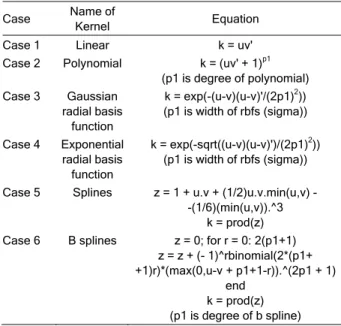
The objective function is minimization of the average absolute relative error (AARE) on the test set and X is a solution string representing a design configuration. The design variable x1 takes any va-lues for C in the range of 0.0 to 10,000. x2 represents the ε taking any values in the range of 0.0 to 1. x3 represents the loss function types: e–insensitive loss function and Huber loss function represented by num-bers 1 and 2 respectively. x4 represents the Kernel types: all 6 kernels given in Table 1 represented by numbers 1 to 6 respectively. The variable x5 takes six values of the kernel parameters (represents the degree of polynomials, etc.) in the range from1 to 6 (1,2,3,4,5,6) represented by numbers 1 to 6.
Table 1. Different kernel type (u and v - kernel arguments)
Case Name of
Kernel Equation Case 1 Linear k = uv' Case 2 Polynomial k = (uv' + 1)p1
(p1 is degree of polynomial) Case 3 Gaussian
radial basis function
k = exp(-(u-v)(u-v)'/(2p1)2)) (p1 is width of rbfs (sigma))
Case 4 Exponential radial basis function
k = exp(-sqrt((u-v)(u-v)')/(2p1)2))
(p1 is width of rbfs (sigma))
Case 5 Splines z = 1 + u.v + (1/2)u.v.min(u,v) - -(1/6)(min(u,v)).^3
k = prod(z) Case 6 B splines z = 0; for r = 0: 2(p1+1)
z = z + (- 1)^rbinomial(2*(p1+ +1)r)*(max(0,u-v + p1+1-r)).^(2p1 + 1)
end k = prod(z) (p1 is degree of b spline)
The total number of design combinations with these variables is 100×100×2×6×6 = 720000. This means that if an exhaustive search is to be performed it will take at the maximum 720000 function evalu-ations before arriving at the global minimum AARE for the test set (assuming 100 trials for each to arrive optimum C and ε). So the strategy which takes few
function evaluations is the best one. Considering the minimization of AARE as the objective function, a dif-ferential evolution technique is applied to find the opti-mum design configuration of the SVR model.
CASE STUDY: THE PREDICTION OF CRITICAL VELOCITY IN SOLID LIQUID SLURRY FLOW
The background and the importance of critical velocity
Compared to a mechanical transport of slurries, the use of a pipeline ensures a dust free environment, demands substantially less space, makes the full au-tomation possible and requires a minimum of the ope-rating staff. The power consumption represents a sub-stantial portion of the overall pipeline transport opera-tional costs. For that reason great attention was paid to the reduction of the hydraulic losses. The predict-tion of critical velocity of slurries and the understand-ing of rhelogical behavior makes it possible to opti-mize the energy and water requirements.
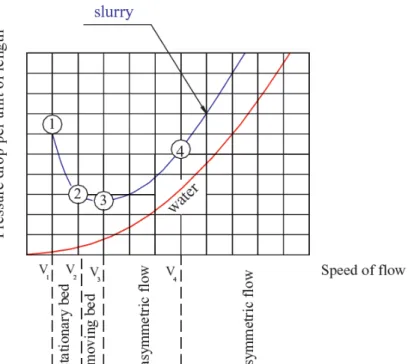
Various investigators [18-20] have tried to show and propose the correlation relating critical velocity with other parameters of the solid-liquid flow, namely solids density, liquid density, particle size, concentra-tion, pipe diameter, viscosity of flowing media, etc. They find that the pressure drop curve passes through minima (point 3 in Figure 2) and the operation at this velocity will ensure the lowest power consumption.
The critical velocity (Vc) is defined as the
mini-mum velocity at which the solids form a bed at the bottom of the pipe demarcating the flow from fully suspended flows. It is also referred to as the minimum carrying or the limiting deposition velocity or the velo-city corresponds to the lowest pressure drop and per-haps the most important transition velocity in a slurry transport. The operation velocities below the critical velocity are uneconomical as the critical velocity rises considerably. Apart from its obvious danger of plug-ging the pipeline, it also produces the excessive ero-sion in the lower part of the pipe. A system containing particles of the wide granulometric range results in the suspension of smaller particles keeping the larger particles deposited in the pipeline. Thus the long term stability of a heterogeneous flow depends on the reli-able prediction of the critical velocity.
The four regimes of the flow can be represented by a plot of the pressure gradient versus the average velocity of the mixture (Figure 2). The critical velocity defined as V3 velocity at or above which all particles
move as an asymmetric suspension and below which the solids start to settle and form a moving bed. For all practical purposes of the slurry transport, the mix-ture velocity is kept above the V3 and thus it is very
Figure 2. The plot of transitional mixture velocity with the pressure drop.
Despite the large area of application, the avail-able models describing the suspension mechanism do not completely satisfy the engineering needs. To facilitate the design and the scale up of pipelines and slurry pumps, there is a need for a correlation that can predict slurry critical velocity over a wide range of operating conditions, physical properties and particle size distributions. The industry needs quick and easily implementing solutions. The model derived from the first principle is no doubt the best solution. But in the scenario where the basic principles for critical velocity modeling accounting all the interactions for slurry flow is absent, the numerical model may be promising to give some quick, easy solutions for the slurry critical velocity prediction.
This paper presents a systematic approach using robust hybrid SVR-DE techniques to build a cri-tical velocity correlation from the available experi-mental data. This correlation has been derived from a broad experimental data bank collected from the open literature (800 measurements covering a wide range of pipe dimensions, operating conditions and physical properties).
The development of the support vector regression (SVR) based correlation
The development of the SVR-based correlation was started with the collection of a large databank. The next step was to perform a support vector regres-sion, and to validate it statistically.
Collection of data
As mentioned earlier, over the years research-ers have simply quantified the critical velocity of the slurry flow in a pipeline. In this work, about 800 expe-rimental points have been collected from 20 sources of the open literature spanning the years 1950-2002. The data were screened for incompleteness, redun-dancies and evident inaccuracies. This wide range of database includes the experimental information from different physical systems to develop a unified corre-lation for critical velocity. Table 2 indicates the wide range of the collected databank for critical velocity.
Table 2. System and parameter studied. Slurry system: coal-water, coal-brine, ash-coal-water, copper ore-coal-water, sand-coal-water, gyp-sum-water, glass-water, gravel-water, iron-water, iron-kerosene, high density material-water, iron tailings-water, limestone-water, limonite-water, plastic-water, potash-brine, sand-ethylene gly-col, nickel shot-water, iron powder-water and ore-water [18,20-30]
Pipe diameter (m) 0.0127–0.80 Particle diameter (m) (0.0017–0.868)×10-2
Liquid density (kg/m3) 770–1350
Solids density (kg/m3) 1150–8900
Liquid viscosity (kg/m-sec) 0.0008–0.19 Solids concentration (volume
fraction) 0.005–0.561
Critical velocity (m/s) 0.18-4.56
Identification of input parameters
Out of the number of inputs in a “wish list”, we used the support vector regression to establish the best set of chosen inputs, which describes the critical velocity. The following criteria guide the choice of the set of inputs:
− The inputs should be as few as possible. − Each input should be highly cross-correlated to the output parameter.
− These inputs should be weakly cross-correla-ted to each other.
− The selected input set should give the best output prediction, which is checked by using statistical analysis (e.g., average absolute relative error (AARE), standard deviation).
While choosing the most expressive inputs, there is a compromise between the number of inputs and the prediction. Based on different combinations of inputs, a trial–and-error method was used to finalize the input set which gives a reasonably low prediction error (AARE) when exposed to the support vector regression.
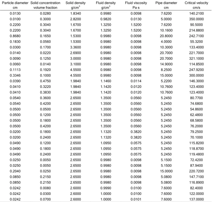
Based on the above analysis, the input variables such as a pipe diameter, a particle diameter, a so-lid(s) concentration, solid and liquid density and vis-cosity of the flowing medium have been finalized to predict the critical velocity in a slurry pipeline (Table 2). Table 3 shows some typical data used for the sup-port vector regression.
Table 3. Typical input and output data for SVR training
Particle diameter cm
Solid concentration volume fraction
Solid density g/cm3
Fluid density g/cm3
Fluid viscosity Pa s
Pipe diameter cm
Critical velocity cm/s
0.0130 0.0280 1.8340 0.9980 0.0098 7.6200 140.2100
0.0100 0.3000 2.8200 0.9820 0.0130 5.0000 350.0000
0.2200 0.3040 1.6700 1.3250 1.5200 7.6200 90.5000
0.2200 0.3040 1.6700 1.3250 1.5200 10.1600 214.8800
0.8680 0.1650 1.5300 0.9980 0.0098 20.8000 242.7100
0.1830 0.0560 1.5300 0.9980 0.0098 4.0000 55.3200
0.0300 0.1700 3.3600 0.9980 0.0098 10.3000 133.4000
0.0140 0.0220 2.6900 0.9980 0.0098 20.7000 221.7000
0.0090 0.1250 3.0000 0.9980 0.0098 20.7000 321.1000
0.0060 0.0140 3.1000 0.9980 0.0098 14.9000 114.8500
0.1113 0.1920 4.5500 0.9980 0.0098 8.2500 247.9200
0.3346 0.1000 4.5500 0.9980 0.0098 15.0000 300.0000
0.0390 0.4750 1.9840 1.1460 0.0114 5.2200 146.3000
0.0410 0.3220 1.9840 1.1420 0.0120 10.7600 123.4000
0.0410 0.3830 1.9840 1.1420 0.0120 10.7600 123.4000
0.0540 0.3600 2.6500 1.3500 0.0560 5.2450 80.7700 0.0540 0.4200 2.6500 1.3500 0.0560 5.2450 74.6800 0.0500 0.0500 2.6500 1.3500 0.0560 5.2450 54.8600 0.0500 0.1200 2.6500 1.3500 0.0560 5.2450 62.4800 0.0500 0.1800 2.6500 1.3500 0.0560 5.2450 68.5800 0.0500 0.4200 2.6500 1.3500 0.0560 5.2450 76.2000 0.0200 0.1800 2.6500 1.1320 0.3820 5.2450 79.2500 0.0200 0.2400 2.6500 1.1320 0.3820 5.2450 70.1000
0.0490 0.1200 2.6500 1.0950 0.0575 5.2450 115.8200
0.0490 0.1800 2.6500 1.0950 0.0575 5.2450 118.8700
0.0490 0.2400 2.6500 1.0950 0.0575 5.2450 119.4800
0.0250 0.0050 2.6500 0.9980 0.0098 5.1500 72.4200 0.0250 0.0050 2.6500 0.9980 0.0098 5.1500 87.9400
0.2040 0.0250 2.6500 0.9980 0.0098 15.0000 220.7200
0.0850 0.2150 2.6500 0.9980 0.0098 5.0800 147.7100
0.0850 0.2150 2.6500 0.9980 0.0098 5.0800 116.8900
0.0242 0.0080 2.6000 0.9990 0.0100 7.6000 82.4000
0.0242 0.0300 2.6000 1.0000 0.0100 7.6000 122.0000
Table 3. Continued
Particle diameter cm
Solid concentration volume fraction
Solid density g/cm3
Fluid density g/cm3
Fluid viscosity Pa s
Pipe diameter cm
Critical velocity cm/s
0.0250 0.3000 2.6500 0.9980 0.0098 10.3000 107.5400
0.0250 0.3180 2.6500 0.9980 0.0098 10.3000 103.5200
0.0400 0.0300 2.6500 0.9980 0.0098 10.3000 347.5000
0.0400 0.0620 2.6500 0.9980 0.0098 10.3000 218.5600
0.0400 0.1370 2.6500 0.9980 0.0098 10.3000 230.4500
0.0242 0.0300 2.6000 1.0000 0.0100 7.6000 122.0000
0.0242 0.0700 2.6000 1.0000 0.0101 7.6000 137.0000
RESULTS AND DISCUSSION
As the magnitude of inputs and outputs greatly differ from each other, they are normalized in -1 to +1 scale by the formula:
min max
min max normal
2
x x
x x x x
− − − =
75 % of the total dataset was chosen randomly for training and the rest 25 % was selected for vali-dation and testing.
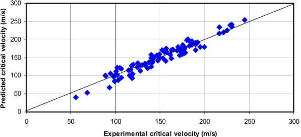
Six parameters were identified as the input (table 2) for SVR and the critical velocity is put as a target. These data were then exposed to hybrid SVR- -DE model described above. After the optimization of five SVR parameters described above, the model out-put was summarized in Table 4. The prediction capa-bility of the hybrid SVR-DE algorithm is plotted in Fi-gure 4. The low AARE (6.5 %) may be considered as an excellent prediction performance considering the poor understanding of the slurry flow phenomena and a large databank for training comprising various sys-tems. The optimum value of SVR meta-parameters were summarized in Table 5. From Table 5 it is clear
that there are almost 5 different feasible solutions which lead to same prediction error.
Table 4. The prediction error by a SVR based model
Parameter Training Testing
AARE 0.0642 0.0645
σ 0.061 0.0625
R 0.940 0.931
In a separate study, we exposed the same data-set to SVR algorithm only (without the DE algorithm) and tried to optimize different parameters based on the exhaustive search. We found that it was not pos-sible to reach the best solutions starting from arbitrary initial conditions. Specially the optimum choice of C
and ε is very difficult to arrive at after starting with some discrete value. Many times the solutions got stuck up in sub optimal local minima. These experi-ments justified the use of a hybrid technique for SVR parameter tuning. The best prediction after the ex-haustive search along with SVR parameters was sum-marized in Table 6. From the Table 6 it is clear that even
0 50 100 150 200 250 300
0 50 100 150 200 250 300
Experimental critical velocity (m/s)
P
re
d
ic
te
d
c
rit
ic
a
l v
e
lo
c
it
y
(
m
/s
)
Table 5. Optimum parameters obtained by hybrid SVR-DE algorithm
Serial No. C ε Kernel type Type of loss function Kernel parameter AARE
1 943.82 0.50 erbf e-Insensitive 2 0.0645
2 2298.16 0.36 erbf e-Insensitive 3 0.0645
3 3954.35 0.48 erbf e-Insensitive 4 0.0645
4 6180.98 0.54 erbf e-Insensitive 5 0.0645
after 720000 runs, the SVR algorithm is unable to locate the global minima and the time of the execution is 4 h in Pentium 4 processor. On the other hand, the hybrid SVR-DE technique is able to locate the global minima with 2000 runs within 1 h. The prediction accuracy is also much better. Moreover, it relieves the non-expert users to choose the different parameters and find the optimum SVR meta parameters with a good accuracy.
Table 6. The comparison of the performance of SVR-DE hybrid model vs. SVR model
Parameter SVR-DE Testing SVR Testing
AARE 0.0645 0.0751
σ 0.0625 0.0655
R 0.931 0.901
Execution time, h 1 4
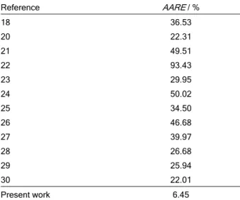
All the 800 experimental data collected from the open literature were also exposed to different formu-las and correlations for critical velocity available in the open literature and AARE were calculated for each of them (Table 7). From Table 7, it is evident that the prediction error of the critical velocity has reduced con-siderably in the present work.
Table 7. The performance of different correlations to predict cri-tical velocity
Reference AARE / %
18 36.53 20 22.31 21 49.51
22 93.43 23 29.95 24 50.02 25 34.50
26 46.68 27 39.97 28 26.68 29 25.94
30 22.01
Present work 6.45
CONCLUSION
The support vector machines regression metho-dology with a robust parameter tuning procedure has been described in this work. The method employs a hybrid SVR-DE approach for minimizing the generali-zation error. Superior prediction performances were obtained for the case study of critical velocity and a comparison with selected correlations in the literature showed that the developed SVR correlation noti-ceably improved the prediction of critical velocity over a wide range of operating conditions, physical proper-ties, and pipe diameters. The proposed hybrid tech-nique (SVR-DE) also relieved the non-expert users to choose the meta-parameters of SVR algorithm for their case study and find out the optimum value of these meta parameters on their own. The results indi-cate that the SVR based technique with the DE based parameters tuning approach described in this work can yield excellent generalization and can be advan-tageously employed for a large class of regression problems encountered in the process engineering.
Nomenclature
α,α*: Vectors of Lagrange’s multiplier ε: Precision parameter
σ: Width of kernel of radial basis function λ: Regularization constant
ζ,ζ*: Slack variables
REFERENCES
[1] V. Vapnik, The Nature of Statistical Learning Theory, Springer Verlag, New York, 1995
[2] V. Vapnik, Statistical Learning Theory, John Wiley, New York, 1998
[3] V. Vapnik, S. Golowich, A. Smola, Adv. Neural Inform. Proces. Syst. 9 (1996) 281
[4] M. Agarwal, A. M. Jade, V. K. Jayaraman, B. D. Kulkarni, Chem. Eng. Prog. 98 (2003) 100
[5] L. B. Jack, A. K. Nandi, Mech. Sys. Sig. Proc. 16 (2002) 372 [6] T. F. Edgar, D. M. Himmelblau, Optimization of Chemical
Processes, McGraw- Hill, Singapore, 1989
[8] K. K. N. Sastry, L. Behra, I. J. Nagrath, Fundamental In-formaticae: Special Issue on Soft Computing (1998) [9] B. V. Babu, K. K. N. Sastry, Comp. Chem. Eng. 23 (1999) 327 [10] C. Burges, Data Mining and Knowl. Disc. 2(2) (1998)
955-975
[11] A. Smola, B. Schölkopf, K. R. Müller, Neural Networks 11 (1998) 637
[12] A. Schölkopf, J. C. Platt, J. Shawe-Taylor, A. J. Smola, R. C. Williamson, Neural Comput. 13 (2001) 1443
[13] V. Cherkassky, F. Mulier, Learning from Data: Concepts Theory and Methods, Wiley, New York, 1998
[14] B Scholkopf, J. Burges, A. Smola, Advances in Kernel Methods: Support Vector Machine, MIT Press, Cam-bridge, MA, 1998
[15] D. Mattera, S. Haykin, Advances in Kernel Methods: Support Vector Machine, MIT Press, Cambridge, 1999 [16] A. J. Smola, B. Schölkopf, K. R. Müller, Neural Networks
11 (1998) 637
[17] T. Hastie, R. Tibshirani, J. Friedman, The Elements of Statistical Learning Data Mining Inference and Prediction, Springer, New York, 2001
[18] R. Durand, E. Condolios, Compterendu des Deuxiemes journees de L Hydraulique, Societe Hydrotechnique de France, Paris, 1952, pp. 29-55
[19] E. J. Wasp, T. C. Aude, J. P. Kenny, R. H. Seiter, R. B. Jacques, Proc. Hydro Transport 1, BHRA Fluid Engi-neering, Coventry, 1970, paper No. H42 53-76
[20] R. G. Gillies, K. B. Hill, M. J. Mckibben, C. A. Shook, Powder Technol. 104 (1999) 269
[21] W. E. Wilson, Trans ASCE 107 (1942) 1576
[22] D. M. Newitt, J. F. Richardson, M. Abbott, R. B. Turtle, Trans. Instn Chem. Eng. 33 (1955) 93
[23] D. G. Thomas, AIChE J. 8 (1962) 373
[24] I. Zandi, G. Govatos, Proc. ACSE, J. Hydraul. Div. 93 (1967) 145
[25] C. A. Shook, The Symposium on pipeline transport of solids, The Canadian society for chemical engineering, Toronto, 1969
[26] H. A. Babcock, Heterogeneous flow of heterogeneous solids. Advances in solid liquid flow in pipes and its ap-plication, Pergamon Press, New York, 1970, pp. 125-148 [27] R. M. Turian, T. F. Yuan, AIChE J. 23 (1977) 232 [28] E. J. Wasp, J. P. Kenny, R. L. Gandhi, Solid liquid flow–
-slurry pipeline transportation, Trans Tech Publ., Rock-port, MA, 1977
[29] A. R. Oroskar, R. M. Turian, AIChE J. 26 (1980) 550 [30] D. R. Kaushal,Y. Tomita, Inter. J. Multiphase Flow 28