A study of the dynamics of quantum correlations

✡ ✪ ✱✱ ✑✑✑ ✟✟ ❡

❡ ❡ ❅

❅_❅ ❧

❧ ❧ ◗

◗◗ ❍ ❍P P P ❳❳ ❳ ❤❤ ❤ ❤

✭ ✭ ✭

✭✏✟✏

_IFT

MASTER DISSERTATION IFT–D.008/2014

A Study of the Dynamics of Quantum

Correlations

Patrice Audibert Camati

Advisor

Dr. Gast˜ao In´acio Krein

Acknowledgements

I, firstly, would like to thank the National Council for Scientific and Technological Development (CNPq) for having granted me with a scholarship along the past two years. I thank my advisor for have accepted me as his student and for have allowed me to pursue my studies in a field which is not one from his expertise. I also must thank some colleagues of mine who provided me with insightful discussions about physics as well as taught me a bit of their respective fields. They are: George De Conto Santos, Guilherme Franzmann, Henrique dos Santos Flores, Lucas Lolli Savi and Marcio Woitek Junior.

“The scientist does not study nature because it is useful; he studies it because he delights in it, and he delights in it because it is beautiful. If nature were not beautiful, it would not be worth knowing, and if nature were not worth knowing, life would not be worth living.”

- HENRI POINCAR´E

“The book of nature is written in the language of mathematics.” - GALILEU GALILEI

“If people do not believe that mathematics is simple, it is only be-cause they do not realize how complicated life is.”

- JOHN VON NEUMANN

“Science is much more than a body of knowledge. It is a way of thinking.”

Abstract

In this work, we present an introduction to the quantum information theory. Before dealing with quantum information we develop some necessary tools, the clas-sical information theory and some important concepts in quantum dynamics. We define measures of quantum correlations, concurrence and quantum discord, and study their dynamical evolution when the coupling between the system and envi-ronment is considered random. We conclude that a random envienvi-ronment imposes permanent loss of correlations to the system.

Key words: Entanglement; quantum discord; random coupling constant.

Resumo

Neste trabalho, apresentamos uma introdu¸c˜ao `a teoria da informa¸c˜ao quˆantica. Antes de lidarmos com a informa¸c˜ao quˆantica propriamente dita, desenvolvemos al-guns assuntos preliminares, a teoria cl´assica da informa¸c˜ao e conceitos relevantes em dinˆamica de sistemas quˆanticos. Depois, definimos medidas de correla¸c˜oes quˆanticas, concorrˆencia e disc´ordia quˆantica, e estudamos sua evolu¸c˜ao dinˆamica quando o acoplamento do sistema com o ambiente ´e modelado como aleat´orio. Conclu´ımos que um ambiente aleat´orio imp˜oe uma perda permanente nas correla¸c˜oes do sistema.

Palavras-chave: Emaranhamento, disc´ordia quˆantica, acoplamento randˆomico.

1 Introduction 1

2 Classical Information Theory 5

2.1 What is information? . . . 6

2.2 Measuring Information . . . 8

2.3 Shannon Entropy . . . 12

2.4 Mutual Information and Other Entropies . . . 17

2.4.1 Relative Entropy . . . 28

3 Quantum Dynamics 31 3.1 Dynamics of Closed Quantum Systems . . . 32

3.1.1 Dynamics of Pure and Mixed States . . . 33

3.1.2 Dynamics of One Qubit . . . 41

3.2 Composite Quantum Systems . . . 47

3.3 Dynamics of Open Quantum Systems . . . 53

3.4 Measurement Dynamics . . . 58

3.5 Generalized Quantum Dynamics . . . 65

3.6 Decoherence and Environment-Induced Superselection . . . 67

4 Quantum Information Theory 73 4.1 The von Neumann Entropy . . . 74

4.2 Entropy at the Interfaces: Preparation and Measurement . . . 81

4.2.1 The Entropy of Projective Measurements . . . 81

4.2.2 The entropy of preparation . . . 83

4.3 Correlations . . . 83

4.4 Measuring Correlations . . . 88

4.4.1 Correlations in Pure States; Entanglement . . . 89

4.4.2 Correlations in Arbitrary Bipartite States; Accounting for Mixed

States . . . 91

4.5 Applications of Quantum Correlations . . . 99

4.5.1 No-Cloning Theorem . . . 100

4.5.2 Quantum Teleportation . . . 102

4.5.3 Entanglement Swapping . . . 105

4.5.4 Quantum Dense Coding . . . 106

4.5.5 Quantum Discord as a Resource . . . 108

5 The Effect of Random Coupling Constants on Quantum Correla-tions 110 5.1 Calculation of the Measures of Quantum Correlations . . . 113

5.2 Numerical Results and Discussions . . . 118

6 Conclusions 129

A Singular Value Decomposition 131

B Operator-Sum Decomposition 135

C Information Theoretic Inequality 138

Introduction

Since the advent of quantum mechanics there has been a huge progress in techno-logy. Quantum mechanics underpins our modern society in many ways, from all kinds of electronic devices to how some economic sectors are structured. One of the new paradigms of technological development is the idea of construct a quantum computer. A computer which exploits in a fundamental way the unique quantum behavior. All computers use quantum mechanics in the sense of using quantum mechanical devices such as the transistor. Nevertheless, when it comes to store and process the information, our current computers use binary language, for example, ei-ther with or without electrical current flowing through the transistors. It is precisely this point that quantum computers intend to extend, by exploiting the superposition property of quantum systems. This story of quantum computers brings us to an-other field greatly developed in the past century, the theory of communication. We will say a few words about information theory in the next chapter. For the moment, let us comment briefly some chain of events that were important for the realization that taking into account quantum mechanics in the way we transmit information can provide more efficient algorithms to some tasks.

Entanglement has been a major concept in modern physics. It is accepted that the first discussion of this property in a scientific article was in the seminal paper written by Einstein, Podolsky and Rosen (also known as EPR article) in 1935 [1]. They questioned if the quantum theory was complete or not. As they were prone to the incompleteness, because in their work this was a consequence if the locality of quantum theory is assumed, they suggested that it might exist hidden variables which would make the quantum theory complete. This means that they have pro-vided an example that seemed to show that quantum mechanics does not respect

locality. The next important step in this story may be considered the work of John S. Bell published in 1964 [2]. Bell set up the discussion to the experimental level. He derived an inequality (called Bell’s inequality) which the supposed (local) hidden variable theory should satisfy. Even though it might have been unclear up to now, all these discussions were raised because since the beginning, with the EPR article, they were dealing with entangled states, those states that seemed to violate locality. Nobody was able to grasp what was really going on at the time. In 1972 John Clauser and Stuart Freedman carried out the first experimental test that Bell’s inequality (and also the Clauser-Horne-Shimony-Holt inequality∗_{) were, in fact, violated by} quantum mechanics. Since then, there has been a myriad of experimental confirma-tion of this feature. The violaconfirma-tion of Bell-like inequalities by quantum mechanics means that there is something fundamentally different that cannot be substituted by the local hidden variable theories, which are the most general notion which preserves both locality and reality (as defined by EPR). It was then that a careful study of such states (those which violate the inequalities) began to grow.

In the early 1980s arose the interest in whether it might be possible to use such quantum effects to signal faster than light. Wootters, Zurek and Dieks [3,4] showed that this is not possible and it turns out that this is prevented by the no-cloning theorem, which says that an arbitrary unknown quantum state cannot be perfectly copied (we will see this in more detail later). This was the first result in quantum mechanics which had a striking distinct characteristic when contrasted with classical information, where bits can be easily copied. In fact, the copying availability is everywhere used in error-correction schemes in classical communication. After that, the field of quantum information began to grow increasingly faster. Right after the discovery of the no-cloning theorem, Bennett and Brassard [5] discovered the first quantum cryptographic protocol, in 1984, representing the beginning of interest in using quantum systems for security of communication. This naturally leads to the will to use quantum mechanics to explore other communication concepts, such as codification, data compression, transmission of information and computation.

With the development of these studies entanglement have found its place. Until recently, it was believed that entanglement was a necessary resource for a quantum

∗_{The CHSH inequality is a Bell-like inequality whose violation by quantum mechanics also}

protocol be more efficient, if that is even the case, than a similar classical protocol which solves the same task. Some quantum protocols will be discussed later in this work, some of which are the quantum teleportation and the super dense coding. Nevertheless, there has been an increasing interest in what is called mixed-state computation. In this computation there is no entanglement, or a negligible amount of entanglement such that it is not the resource that promote the efficiency of the algorithm. These resources are still somewhat fundamentally quantum, although there is much more research ahead for clarification of this issue. One example of another resource, other than entanglement, is quantum discord, which we are also going to discuss and show an efficient quantum algorithm to solve a task that there is no known classical algorithm that does so. These quantum correlations are indeed playing the role of potential resources for speedup computation, justifying the interest on studying them.

This work has two aims. First, it is structured to provide an introduction to quantum information theory, beginning with a review of the major concepts of classical information theory and quantum mechanics, although there were some issues that were just commented and an appropriate explanation was left behind. Second, it serves to present an analysis about the behavior of some measures of quantum correlations when the coupling constant between system and environment is random.

Classical Information Theory

Information theory is a broad field of science which comprises applied mathe-matics, electrical engineering and computer science [6]. The landmark work that may be considered as the starting point of the information theory is the article en-titled “A Mathematical Theory of Communication”, written by Claude E. Shannon in 1948 [8]. Shannon was a researcher at the Math Center at the Bell Laboratories, a division created by the American Telephone and Telegraph (AT&T) specifically for conducting research and development of communication systems. From a fairly reasonable set of properties that an appropriate measure of information should have, he arrived at a function, which he himself recognized as being similar to the sta-tistical entropy, that properly measures information, choice and uncertainty. This function is the so-called Shannon entropy.

Information theory is not concerned with the meaning of the information sent, but with practical issues such as how to send efficiently and reliably a signal through a noisy channel such that it can be recovered faithfully. The development of this field enabled the invention of the Internet, which certainly is one of the technolog-ical achievements that most shaped, and still is powerfully capable of shaping, our modern society.

The aim of this chapter is to present an introduction to the classical information theory, going through its fundamental concepts, all of which will be of key impor-tance when we turn into the quantum information theory. We will not be concerned with actual applications.

The structure of this chapter is the following. In Sec. 2.1 we will discuss the concept of information, making the meaning of the word clear when we use it. Following this, we will reach at an objective meaning of information, thus enabling

us to quantify it and use it operationally. Encouraged by this meaning, in Section 2.2, we will study a measure of information supported by it. In Section 2.3 we will explore the fundamental concept of information theory, the Shannon entropy. Instead of being concerned with the actual derivation given by Shannon, we will present it as a definition and work with it in some examples to understand its meaning. In Section 2.4 we will begin to explore the correlations between two or more messages. In order to do so we will use other entropies, namely, the joint entropy, the conditional entropy, the mutual information and the relative entropy. These entropies rest upon the Shannon entropy and are as important as the Shannon entropy itself. The quantum analogous of some of these entropies will give us a measure of quantum correlations.

The presentation is intended to be pedagogical, as a solid understanding of the concepts of information theory in the classical case is important when one goes to the quantum case.

This chapter is heavily based on the Ref. [7].

2.1

What is information?

If we wonder about the concept of information for while it is not difficult to realize that it has many facets. In fact, it is not such a rare insight to realize that define any abstract noun as precise as possible is by no means an easy task. Semantics, the field of Linguistics that studies the meaning of words, phrases, et cetera, is a very interesting subject. Studying how we acquire the meaning of words shows us that from our early days we learn based on our experience. Our brain is biologically adapted to learn languages. We observe the behavior of those around us, listen to those mysterious sounds they make and by simply being there our brain is able to connect those sounds with the present situation and, even though it is an extremely complex process, after two or three years we are able to produce, identify precisely and understand those sounds and their meanings [9]. Based on this phenomenon the present author believes the best way to define a concept, mainly an abstract one, is heuristically. We will go through a couple of situations where the idea of information is applied and then reflect about its different meanings.

neighbors and live side by side in such a way that from Alice’s bedroom window she can see Bob’s bedroom window and vice versa. They have established a secret code using a lantern. If Alice flashes once, it means that her parents have left home. If Alice flashes twice, it means that her parents have decided not to go out anymore. Without minding why they would like to communicate with each other, this situation brings us the opportunity to explore the concept of information. We say that after Alice flashed once or twice, Bob has received information from her. So, one property of informatioin is that it can be transmitted. The code they established must be knowna priori to both Alice and Bob. If Bob didn’t know about the code, he would have not been able to read the message properly. He simply would not have understood it. The abstract message, either parents at home or not, had to be coded in a physical system. In the present case, the flashes of light. Moreover, if it was not a problem, Alice could have just yelled at him. The very same information would have been transmitted through another physical system, namely, the sound waves in the air. Thus, the same information can be stored in different physical systems.

even say that he had been listening inattentively or uninterestedly until the moment when Alice told him something new, unexpected. He, then, might have turned his attention on her to listen carefully the details which were new to him. This is the key. We measure information as how unexpected, uncertain, unpredictable something is. The more uncertain, unexpected, unpredictable something is the more information we will gain when we acquire that knowledge. We will make these concepts more precise in the sections to follow.

With this sense, we have a proper lead to an objective (and hence scientifically useful) definition of information because in order to use it we must have an opera-tional definition. Something we can manipulate and calculate mathematically.

To summarize this section, we concluded that information is something that can be coded, transmitted, copied and stored in different ways. The scientific concept which we will develop from now on will not be concerned with the meaning of the words or symbols, because this is a subjective property from which we can not make science. Instead, we will measure information based on unexpectancy, uncertainty and unpredictability.

2.2

Measuring Information

The focus of this section is to develop a measure of the amount of information. We concluded the last section realizing that we measure information qualitatively relating the knowledge of some event as how much unexpected or unpredictable it is. The most unexpected the event is the more surprised we will be while acquiring that knowledge and consequently more information we gain.

We may assume, for instance, that

p(W) = 0.000001, (2.1)

p(L) = 0.999999. (2.2)

Now the question is, how much information does Alice get when actually knowing the lotto result? As we know from our experience that the odds of winning are small, so does Alice. Therefore she has not much expectation of winning, she will not learn much upon realizing that she has, indeed, lost. But on the contrary case, if she wins, it would be quite a surprise for her (as it would be for us). There is a lot of information in the winning event, to the same extent there is little information in the losing event. Now we have to find a proper mathematical function to measure the information. This function must obey some conditions. This function, call it

I(x) , should approach zero for events closed to absolute certainty, and infinity for events reaching the impossibility. It must also satisfy that I(x1)> I(x2) if the two

events satisfyp(x1)< p(x2), meaning that the less likely event is associated with the

greater information. An information measure that satisfies all these requirements is the following

I(x) = ₋Klog [p(x)], (2.3)

where log(x) is the base two logarithm and K is a dimensionless constant which we will set up to 1 for the moment and later we shall see why this is appropriate. In our lotto example we have

I(W) = ₋log [0.000001] = 19.9315686, (2.4)

I(L) = ₋log [0.999999] = 1.0_×10−6. (2.5)

As expected by construction, the winning event has more information because it is more unexpected.

an unbiased coin there is a probability of one half to get either heads or tails. Hence

p(heads) = p(tails) = 1/2. The information associated with each of these events is I(heads) =I(tails) = 1 bit. Therefore what a bit means is the exact amount of information necessary to describe the outcome of a coin tossing. This is why we had set up, by convention, the constantK in Eq. (2.3) to 1: to match up the scale of the measure with the simplest case. The logarithmic function can again be seen to be appropriate as it fits our intuition that if we had two coins the amount of information needed to describe the outcome of both coins would be doubled. For instance, we would have p(heads,heads) = p(heads,tails) =p(tails,heads) =p(tails,tails) = 1/4 and therefore I(heads,heads) =I(heads,tails) =I(tails,heads) =I(tails,tails) = 2 bits.

Let us now apply this measure in another situation. Consider an unbiased dice. The possible outcomes of rolling a dice are X =_{1,2,3,4,5,6_}. The probability of each event is p(x= 1) =_{· · ·}=p(x= 6) = 1/6. The amount of information in each outcome is, therefore,

I(X) = ₋log (1/6)_≈2.584 bits. (2.6)

The above result may seem confusing at first sight. How do we interpret a real amount of information? The meaning of this result is that we need a string of at least 3 symbols to code all possible outcomes unambiguously. Using a string of length 3 we can code the outcomes as: 1 = 001, 2 = 010, 3 = 011, 4 = 100, 5 = 101 and 6 = 110. Note that we are also left with two possible blocks: 000 and 111. Even though the coding is arbitrary, for any coding of length three, there will remain two blocks unused.

There is an alternative interpretation for the amount of information measured in bits: an operationally one. The logical truth values YES and NO can be thought of as a binary alphabet. This alphabet may be interpreted as the answer (outcome) of a YES-or-NO question. How many questions do we need to ask in order to know the outcome of a coin tossing? One question may be: is the result 0? If yes, then we already know the result. If no, by complementarity we know that the result was 1†_. Therefore, there exists exactly one YES-or-NO question such that when answered

†_{We could have asked about the outcome 1, i.e., it might exist more than one appropriate}

we know the result unambiguously. The existence of exactly one question is directly associated with the amount of information which is, in this case, 1 bit. In the dice rolling we have 6 equiprobable outcomes. How many questions do we need to ask in order to know the outcome of a dice rolling? The first question which comes to mind is, like before: is the result 3 (or any other)? If the answer is yes then we know the result. If it is no we don’t. This is a difference between the coin tossing and the dice rolling. In the coin tossing example, there are only two possible outcomes. So, one such question is enough to know the outcome with certainty. But this is not the case in the dice rolling because it does not have only 1 bit of information. Only with questions of the kind “is the outcome of the dice rolling x ?” we would need six questions to know the outcome with certainty. Let us try to find a small set of questions which unambiguously gives the result when answered. Consider the three following questions:

1. Is the result x even? If YES, then x ∈ {2,4,6} = U1, if NO,

then x_{∈ {}1,3,5_}=U2.

2. Is the resultx strictly greater than 3? If YES, then x_{∈ {}4,5,6_}=V1, if NO,

then x∈ {1,2,3}=V2.

3. Is the result x divisible by 3? If YES, then x ∈ {3,6} = W1, if NO,

then x_{∈ {}1,2,4,6_}=W2.

When these questions are answered they yield precisely the value of x:

• {1_}=U2∩V2 ∩W2 ,i.e., 1 = NO/NO/NO;

• {2_}=U1∩V2 ∩W2 ,i.e., 1 = YES/NO/NO;

• {3_}=U2∩V2 ∩W1 ,i.e., 1 = NO/NO/YES;

• {4_}=U1∩V1 ∩W2 ,i.e., 1 = YES/YES/NO;

• {5_}=U2∩V1 ∩W2 ,i.e., 1 = NO/YES/NO;

• {6_}=U2∩V2 ∩W2 ,i.e., 1 = YES/YES/YES.

Note again that there are two combinations that are not used, YES/NO/YES (U1∩

of the binary symbols YES and NO out of eight possible ones. This is why the informational content of the dice rolling is between 2 and 3. If the source was given by eight equiprobable symbolsY ={1,2,3,4,5,6,7,8}=X∪{7,8}we would have 3 bits of information because each symbol would have probability 1/8. What does the differenceI(Y)−I(X) = 0.416 mean? Well, it is exactly the amount of information which we gain from source Y when it is no longer equiprobable because its two last symbols have now (from the point of view of the source X) zero probability of occurrence. This excess of probability are redistributed among the other six symbols to form a new source of equiprobable six symbols, namely, X. Each of these six symbols will have their probabilities increased by 8/6 which in terms of information means I(∆Y) = −log (8/6) = −0.416. After this re-arrangement the new source has information I(X) =I(Y) +I(∆Y) = 3₋0.416 = 2.584 bits. This supports the interpretation of information as being related to certainty. If there are two symbols that do not show up anymore then we are more certain about the possible outcomes (because we have eliminated two possibilities) and therefore less information is associated.

Summarizing this section, we have seen that the simplest alphabet is composed by the binary digits (bits) 0 and 1 (or YES and NO, or whichever). The measure of information I(x) is dimensionless and its common unit is the bit. The amount of information of a given event, as measured by I(x), is a positive real number. In terms of coding the information in bits, the shortest string of bits to code an event, or a message, of information I(x) is given by the smallest n such that n_≥I(x).

2.3

Shannon Entropy

reliably after the transmission. These motivated him to seek an improved measure of information. From a small set of hypotheses that this measure should obey he deduced mathematically a function which he called entropy. We are not going to discuss the hypotheses made by Shannon or how he arrived at the expression of this entropy. Instead, we are going to define it and apply it to some examples in order to grasp its meaning because this is what is important when we turn our attention to quantum information theory in Ch. 4.

It turns out that the Shannon entropy (also called source entropy∗_{) is given by} the average of the information measure we have been studying so far, i.e.,

H(X) =_hI(x)_i=₋X

x∈X

p(x) logp(x). (2.7)

The entropy of a source is, therefore, the average amount of information per source symbol. If the source is equiprobable then the source entropy reduces to the infor-mation, i.e.,

H(X) = −X x∈X

p(x) logp(x) = − N

X

i=1

1

N log

1

N = logN. (2.8)

This means that we have been working with the Shannon entropy all along but in a special case. If we use the base two logarithm then the unit of the entropy is bit/symbol.

The entropy of a dice roll is

H(X) = log 6 = 2.584 bit/symbols, (2.9)

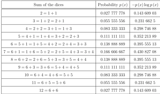
which is the same as the amount of information found in Eq. (2.6) because of the equiprobability of the events, as stated above. Let us consider that we throw two dices in a row and we want to study the sum of the two outcomes. Hence the outcomes of this new source are X = _{2,3,4,5,6,7,8,9,10,11,12_}. Table 2.1 accounts for the probabilities of each of these events. With the data of the table we can evaluate the source entropy, which is found to be H(X) = 3.274 bits/symbol. This means that, on average, each event can be described through a number of bits between 3 and 4, which is expected since we have 11 symbols to represent and 4 bits ↔ 24 _{= 16 > 11 > 8 = 2}3 _{↔ 3 bits. As physically there is no such thing of}

∗_{The concept of a source is going to be addressed later on. For now it is enough to say that a}

Sum of the dices Probabilityp(x) ₋p(x) logp(x) 2 = 1 + 1 0.027 777 778 0.143 609 03 3 = 1 + 2 = 2 + 1 0.055 555 556 0.231 662 5 4 = 2 + 2 = 3 + 1 = 1 + 3 0.083 333 333 0.298 746 88 5 = 4 + 1 = 1 + 4 = 3 + 2 = 2 + 3 0.111 111 111 0.352 213 89 6 = 5 + 1 = 1 + 5 = 4 + 2 = 2 + 4 = 3 + 3 0.138 888 889 0.395 555 13 7 = 6 + 1 = 1 + 6 = 5 + 2 = 2 + 5 = 4 + 3 = 3 + 4 0.166 666 667 0.430 827 08 8 = 6 + 2 = 2 + 6 = 5 + 3 = 3 + 5 = 4 + 4 0.138 888 889 0.395 555 13 9 = 6 + 3 = 3 + 6 = 5 + 4 = 4 + 5 0.111 111 111 0.352 213 89 10 = 6 + 4 = 4 + 6 = 5 + 5 0.083 333 333 0.298 746 88 11 = 6 + 5 = 5 + 6 0.055 555 556 0.231 662 5

12 = 6 + 6 0.027 777 778 0.143 609 03

Table 2.1: Probabilities of the summation of the outcomes of rolling two dices. This table was trascripted from Ref. [7].

rational binary symbols we need four bits to code the outcomes of this source. As in the case considered in Sec. 2.2 we will be left with possible coding blocks unused whichever coding we perform.

There is a nice operational interpretation of the Shannon entropy which we will address in the following [10], but a small reflection at this point is worthy.

As we have discussed in Sec. 2.1, for all practical purposes we don’t have interest in the meaning of the messages. We want to study the properties of messages in an objective way. In fact, we have already been doing this when we treated the coin tossing and the dice rolling. Let us think about the kinds of messages we are used to in daily life. Texts in any human language are a complex structure made of sentences, words, letters, syntactic rules, et cetera. Furthermore, exactly because of this complex structure, the probability of a given letter occur within a string of letters (and spaces) depends on the word it finds itself in. Therefore, in order to measure the information that a new letter would have if it filled in the next position in the string we would need to consider too many joint and conditional probabilities. Let us forget that these complications exist and study a relatively simple source and see what we can learn from it.

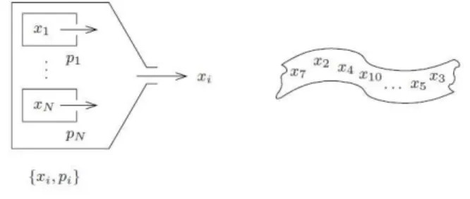
sequential manner. The probability pi of the letter xi occur in a given position of

the sequence is completely uncorrelated with what has already been written or will be written. This machine is called a signal source without memory and the set

{xi, pi}is called signal ensemble† (see Fig. 2.1). From now on a message is going to

be a definite sequence of n letters generated by this kind of machine.

Figure 2.1: Representation of the signal source with signal ensemble _{xi, pi}. This

figure was copied from Ref. [10]

Alice uses this printing machine to send messages to Bob. She doesn’t send the message as a whole but letter by letter. Therefore, Bob does not know what letter may come next but he does know the signal ensemble. Remember our discussion in Sec. 2.1, Bob did know the code.

Consider that Alice prints out a sequence ofnletters. If the alphabet containsN

different letters, then there areNn _{such sequences. The relative frequency of a letter} xi to appear in these sequences is of the ordernpi. With a large enough sequence the

frequency of a letterxi may be considered ni =npi. A sequence such asxixi. . . xi is

not excluded but has a probability pn

i, which is very small since 0≤pi ≤1 andn is

large. So, when n is sufficiently large, Bob may assume that he will only receive the sequences which contain the letters xi’s with the frequencies ni’s. These sequences

are called typical sequences. A fairly reasonable question is: how many of these sequences are there? Well, there aren! ways to arrange the n letters. Permutations of the same letter in a sequence does not change it. As there are ni occurrences of

the letterxi we need to remove theni! possible permutations. Hence the number of

typical sequences is

Zn =

n!

n1!n2!. . . nN!

. (2.10)

Using the Stirling’s formula log (n!)≈nlogn−n, which is valid whenn is large, we obtain for the logarithm of Zn

logZn≈nlogn−n− N

X

i=1

(nilogni−ni) =−n N

X

i=1

pilogpi. (2.11)

If we divide this by n and take the limitn→ ∞ we obtain the Shannon entropy

H(X) := lim

n→∞

1

n logZn =− N

X

i=1

pilogpi. (2.12)

Or equivalently

Zn= 2nH(X)(asymptotically). (2.13)

Since many (few) possibilities reflect a large (small) measure of a priori uncer-tainty for Bob,H(X) from Eq. (2.12) is a measure of the meana priori uncertainty of a character which is received by Bob. Then H is at the same time the average information which Bob receives per transmitted character. This result is a simplified way of stating the Shannon’s source coding theorem.

As we said previously the simplest source is composed by two bits. Let us calculate the Shannon entropy for this source. The Shannon entropy is simply

H(X) = ₋plogp₋(1₋p) log (1₋p), (2.14)

where pis the probability to get the bit 0, for example. This function is also called binary entropy function and it is plotted in Fig. 2.2.

We see that the Shannon entropy has a maximum, when the two bits have the same probability of occurrence, namely, 1/2, and it has two minima, when one of the bits has certainty of occurrence. The maximum situation is the one which we are more uncertain about the next symbol given by the source. Exactly because there is the same probability to occur either 0 or 1, there is no way to discriminate. As the probability of one symbol is increasing, the entropy is reduced because we know that one symbol occurs more frequently than the other. The extreme case is when the source just prints out one symbol. In this case we are completely certain of the next symbol and therefore the entropy reaches zero.

0 0.1 0.2 0.3 0.4 0.5 0.6 0.7 0.8 0.9 1

0 0.1 0.2 0.3 0.4 0.5 0.6 0.7 0.8 0.9 1

Shannon entropy

probability p

Figure 2.2: Shannon entropy for a 1-bit source.

2.4

Mutual Information and Other Entropies

We have been discussing about events, messages, random variables, information and entropy. Both information and entropy are quantities which depend on one message (or one random variable). In this chapter we shall deal with other entropies, all of which tell us about the correlations between two (or more) messages. We shall answer questions like: How much information do these two messages share in common? How much information do I gain reading this message given I’ve read the other? As we shall see in Ch. 4 these entropies play a central role in quantum information theory. We will consider a concrete example and define these entropies as we go through.

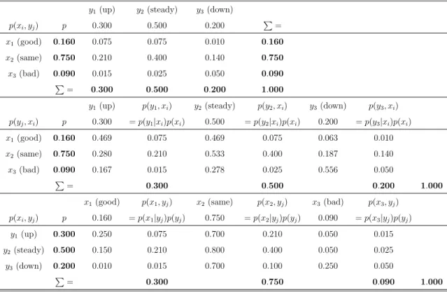
Consider two event sources related with a public company [7]. The first event source is about three possible conclusions for the quarterly sales report, namely

x ∈ X = {good,same,bad} = {x1, x2, x3}, meaning that the results are in excess

of the predictions (good), or on target (same), or under target (bad). The second event source is the company’s stock value, as reflected by the stock exchange, with

y_∈Y =_{up,steady,down_}=_{y1, y2, y3}. Then assume that there exists some form

y1(up) y2 (steady) y3(down)

p(xi, yj) p 0.300 0.500 0.200 P=

x1(good) 0.160 0.075 0.075 0.010 0.160

x2(same) 0.750 0.210 0.400 0.140 0.750

x3(bad) 0.090 0.015 0.025 0.050 0.090

P_{= 0.300 0.500 0.200 1.000}

y1(up) p(y1, xi) y2(steady) p(y2, xi) y3(down) p(y3, xi)

p(yj, xi) p 0.300 =p(y1|xi)p(xi) 0.500 =p(y2|xi)p(xi) 0.200 =p(y3|xi)p(xi)

x1(good) 0.160 0.469 0.075 0.469 0.075 0.063 0.010

x2(same) 0.750 0.280 0.210 0.533 0.400 0.187 0.140

x3(bad) 0.090 0.167 0.015 0.278 0.025 0.556 0.050

P

= 0.300 0.500 0.200 1.000

x1(good) p(x1, yj) x2(same) p(x2, yj) x3(bad) p(x3, yj)

p(xi, yj) p 0.160 =p(x1|yj)p(yj) 0.750 =p(x2|yj)p(yj) 0.090 =p(x3|yj)p(yj)

y1(up) 0.300 0.250 0.075 0.700 0.210 0.050 0.015

y2 (steady) 0.500 0.150 0.210 0.800 0.400 0.050 0.025

y3(down) 0.200 0.010 0.015 0.700 0.100 0.250 0.050

P

= 0.300 0.750 0.090 1.000

Table 2.2: Numerical example of the quarterly sales report and the company’s stock value sources. This table was trascripted from Ref. [7].

numerical example of joint and conditional probability data, p(xi, yj), p(xi|yj) and p(yj|xi) is shown in Table 2.2.

The first group of numerical data, shown at the top of Table 2.2, corresponds to the joint probabilities p(xi, yj). Summing up the data by rows (i) or by columns (j)

yields the probabilities p(xi) orp(yj), respectively. The double checksum (bottom

and right) which yields unity through summing by row or by column is also shown for consistency. The two other groups of numerical data in Table 2.2 correspond to the conditional probabilitiesp(xi|yj) andp(yj|xi). These are calculated through Bayes’

rule p(xi|yj) = p(xi, yj)/p(yj) and p(yj|xi) = p(xi, yj)/p(xi). The intermediate

columns providing the data p(xi|yj)p(yj) = p(yj|xi)p(xi) = p(xi, yj) and their

checksums by column are shown in the table for consistency.

We define the joint entropy H(X, Y) associated with the joint distribution

p(x, y),with x∈X and y ∈Y, as

H(X, Y) = ₋X

x∈X

X

y∈Y

p(x, y) logp(x, y). (2.15)

probability distribution. This entropy represents the average information derived from joint events occurring from two sources X and Y. The unit of H(X, Y) is bit/symbol.

We then define the conditional entropy H(X_|Y) through

H(X|Y) =−X x∈X

X

y∈Y

p(x, y) logp(x|y). (2.16)

The conditional entropyH(X|Y) corresponds to the average information conveyed by the conditional probability distribution p(x_|y). Put simply, H(X_|Y) represents the information we learn from source X given the information we have from source

Y. Its unit is also bit/symbol.

Note that in the joint and conditional entropy definitions the two-dimensional averaging over the event space _{X, Y_} consistently involves the joint distribution

p(x, y).

The conditional entropy H(Y_|X) is defined in the same way, namely,

H(Y_|X) =₋X

x∈X

X

y∈Y

p(x, y) logp(y_|x). (2.17)

As the conditional probabilities p(x_|y) and p(y_|x) are in general different, the two conditional entropies will also be different.

If the two sources are statistically independent then p(x, y) = p(x)p(y). Con-sequently, this implies that

H(X, Y) =₋X

x∈X

X

y∈Y

p(x, y) logp(x, y)

=₋X

x∈X

p(x) logp(x)₋X

y∈Y

p(y) logp(y) =H(X) +H(Y). (2.18)

Moreover p(x_|y) =p(x), then

H(X|Y) = −X x∈X

X

y∈Y

p(x, y) logp(x|y)

=₋X

x∈X

p(x) logp(x) X

y∈Y p(y)

!

=H(X) (2.19)

and

H(Y_|X) =₋X

x∈X

X

y∈Y

p(x, y) logp(y_|x)

=−X y∈Y

p(y) logp(y) X

x∈X p(x)

!

These results match with our intuition that if the two sources are statistically in-dependent the knowledge of one of them does not provide any advance knowledge about the other.

In the general case where the sources are not necessarily statistically independent we find a relation between the joint and conditional entropies given by

H(X, Y) = ₋X

x∈X

X

y∈Y

p(x, y) logp(x, y)

=₋X

x∈X

X

y∈Y

p(x, y) logp(x_|y)₋X

y∈Y

p(y) logp(y)

=H(X|Y) +H(Y), (2.21)

or equivalently,

H(X, Y) = ₋X

x∈X

X

y∈Y

p(x, y) logp(x, y)

=₋X

x∈X

X

y∈Y

p(x, y) logp(y_|x)₋X

x∈X

p(x) logp(x)

=H(Y_|X) +H(X). (2.22)

These expressions may be easier to memorize under the forms

H(X|Y) =H(X, Y)−H(Y), (2.23)

H(Y|X) =H(X, Y)−H(X), (2.24)

which state that, given a source X (Y), any advance knowledge from the other sourceY (X) reduces the joint entropyH(X, Y) by the net amountH(Y) (H(X)), respectively. It will be shown in Sec. 2.4.1 that all these quantities are positive. In other words, the prior information one may gain from a given source is made at the expense of the information available from the other source, unless the two are statistically independent.

We can illustrate the above properties through our stock-exchange probability distributions’ data from Table 2.2. We want, here, to determine how the average in-formation from the company’s sales,H(X), is affected by that concerning the stocks,

H(Y), and vice versa. The computations ofH(X), H(Y), H(X, Y), H(X|Y) and

ui=p(xi)

vj=p(yj)

ui −uilogui vj −vjlogvj

x1(good) 0.160 0.423 y1(up) 0.300 0.521

x2(same) 0.750 0.311 y2(steady) 0.500 0.500

x3(bad) 0.090 0.313 y3(down) 0.200 0.464

H(X) = 1.0469 H(Y) = 1.4855

H(X) + H(Y) = 2.5324

uij=p(xi, yj)

ui1 −ui1logui1 ui2 −ui2logui2 ui3 −ui3logui3

x1 0.075 0.280 0.075 0.280 0.010 0.066

x2 0.210 0.473 0.400 0.529 0.140 0.397

x3 0.015 0.091 0.025 0.133 0.050 0.216

P_{= 0.844} P_{= 0.942} P_{= 0.680}

H(X, Y) = 2.4657

vji=p(yj|xi)

v1i ui1 −ui1logv1i v2i ui2 −ui2logv2i v3i ui3 −ui3logv3i

x1 0.469 0.075 0.082 0.469 0.075 0.082 0.063 0.010 0.040

x2 0.280 0.210 0.386 0.533 0.400 0.363 0.187 0.140 0.339

x3 0.167 0.015 0.039 0.278 0.025 0.046 0.556 0.050 0.042

P

= 0.506 P

= 0.491 P

= 0.421

H(Y|X) = 1.4188

wij=p(xi|yj)

w1j u1j −ui1logw1j w2j u2j −ui2logw12 w3j u3j −u31logw3j

y1 0.250 0.075 0.150 0.700 0.210 0.108 0.050 0.015 0.065

y2 0.150 0.075 0.205 0.800 0.400 0.129 0.050 0.025 0.108

y3 0.050 0.010 0.043 0.700 0.140 0.072 0.250 0.050 0.100

P

= 0.398 P

= 0.309 P

= 0.421

H(X|Y) = 0.9802

H(X, Y) = H(Y|X) + H(X)

2.4657 = 1.4188+ 1.0469

= H(X|Y) + H(Y)

= 0.9802+ 1.4855

qwe

easier reading, we omit here the bit/symbol units). The joint entropy is found to be

H(X, Y) = 2.466, which is lower than the sumH(X) +H(Y) = 2.532. This proves that the two sources are not independent, namely, that they have some information in common. We find that the conditional entropies satisfy

H(Y|X) = 1.418< H(Y) = 1.485, (2.25)

H(X|Y) = 0.980< H(X) = 1.046, (2.26)

or equivalently, using four decimal places, for accuracy (see Fig. 2.3)

H(Y)−H(Y|X) = 1.4855−1.4188 = 0.0667, (2.27)

H(X)−H(X|Y) = 1.0469−0.9802 = 0.0667. (2.28)

These two results mean that the prior knowledge of the company’s stocks contain an average of 0.0667 bit/symbol of information on the company’s quarterly result, and vice versa. As we shall see below, the two differences above are always equal and they are called mutual information. Simply put, the mutual information is the average information that two sources share in common.

We can define the mutual information of two sourcesX andY as the bit/symbol quantity

H(X;Y) = X

x∈X

X

y∈Y

p(x, y) log p(x, y)

p(x)p(y). (2.29)

We may note the absence of a minus sign in the above definition, unlike inH(X, Y),

H(Y_|X) and H(X_|Y). Also note the “;” separation, which distinguishes mutual information from joint entropy H(X, Y). Mutual information is also often referred to in the literature as I(X;Y) instead of H(X;Y).

Since the logarithm argument is unity when the two sources are statistically independent, we immediately observe that the mutual information is equal to zero in this case. This reflects the fact that independent sources do not have any information in common.

It is pertinent, now, to derive some formulas which relate these different en-tropies. Using the properties of the logarithmic function, the Bayes’ rule and the relations P

xp(x, y) = p(y) and

P

distri-bution, the mutual information can be written in the following ways

H(X;Y) = X

x∈X

X

y∈Y

p(x, y) log p(x, y)

p(x)p(y)

=₋X

x∈X

p(x) logp(x) +X

x∈X

X

y∈Y

p(x, y) logp(x_|y)

=H(X)₋H(X_|Y), (2.30)

H(X;Y) = X

x∈X

X

y∈Y

p(x, y) log p(x, y)

p(x)p(y)

=₋X

y∈Y

p(y) logp(y) +X

x∈X

X

y∈Y

p(x, y) logp(y_|x)

=H(Y)−H(Y|X) (2.31)

and

H(X;Y) =H(X) +H(Y)₋H(X, Y), (2.32)

where in the last formula one can use either Eq. (2.30) or Eq. (2.31) together with Eqs. (2.23). The first two equalities above confirm the observation derived from our previous numerical example. They can be interpreted according to the following statement: mutual information is the reduction of uncertainty inX that we get from the knowledge of Y (and vice versa).

The last equality, as rewritten under the form

H(X, Y) =H(X) +H(Y)₋H(X;Y), (2.33)

shows that the joint entropy of two sources is generally less than the sum of the source entropies. The difference is the mutual information that the sources have in common, which reduces the net uncertainty or joint entropy.

Finally, we note from the Eqs. (2.30), (2.31) and (2.32) that the mutual infor-mation is symmetrical with respect to its arguments, namely,H(X;Y) =H(Y;X), as is expected from its very meaning.

ensembles may or may not have elements in common. The set of common elements is calledG=A_∩B (AintersectionB). The same definitions of union and intersection apply to any three ensembles A, B, and C. Fig. 2.3 shows the Venn diagram representations of such ensemble combinations. In the case of two ensembles, there exist four subset possibilities, as defined by their elements’s properties:

• Elements common to A orB: A_∪B,

• Elements common to A and B: A∩B,

• Elements fromA and not B: A∩ ¬B,

• Elements fromB and not A: B_{∩ ¬}A.

Figure 2.3: Venn diagram representation of two (top) and three (bottom) ensem-bles.This figure has been taken from Ref. [7].

logical NO. These three different symbols, which are also called Boolean operators∗_, make it possible to perform various mathematical computations in the field called Boolean logic. In the case of three ensembles A, B, C, we observe that there exist many more subset possibilities (e.g.,A_∩B_∩C,A_∩B_∩¬C). The interest of the above visual description with the Venn diagrams is the straightforward correspondence with the various entropies that have been introduced. Based on Eqs. (2.18), (2.19), (2.20), (2.23), (2.30), (2.31) and (2.32) we can draw a Venn diagram which respects them and see that the following equivalences hold (compare Fig. 2.3 with Fig. 2.4):

         

        

H(X, Y)↔H(X∪Y)

H(X;Y)↔H(X∩Y)

H(X|Y)↔H(X∩ ¬Y)

H(Y|X)↔H(¬X∩Y)

(2.34)

The first equivalence in Eq. (2.34) means that the joint entropy of two sources is the entropy of the source defined by their combined events. The second equivalence in Eq. (2.34) means that the mutual information of two sources is the entropy of the source containing the events they have in common. The last two equivalences in Eq. (2.34) provide the relationship with the conditional entropy. For the case of the conditional entropy of a source X given the information on a source Y, the conditional entropy is given by the contributions of all the events belonging to X but not to Y. Fig. 2.4 illustrates all the above logical equivalences through Venn diagrams, using up to three sources. Considering the two-source case, we can immediately visualize from Fig. 2.4 to which subsets the differences H(X)₋

H(X;Y) and H(Y)₋H(X;Y) actually correspond. Given the identities listed in Eq. (2.34), we can call these two subsetsH(X_|Y) andH(Y_|X), respectively, which proves the previous point. We also observe from the Venn diagram thatH(X|Y)≤ H(X) and H(Y_|X)_≤H(Y), with equality if the sources are independent.

The above property can be summarized by the statement according to which conditioning reduces entropy. A formal demonstration, using the concept of “relative entropy” is provided later.

The three-source case, as illustrated in Fig. 2.4, is somewhat more tricky because ∗_{These are not exactly the symbols which usually represent the Boolean operators but this is}

Figure 2.4: Venn diagram representation for the different entropies.This figure has been taken from Ref. [7].

it generates more complex entropy definitions with three arguments X, Y, and

Z. Conceptually, defining joint or conditional entropies and mutual information with three (or more) sources is not that difficult. Considering the joint probability

p(x, y, z) for the three sources, we can indeed generalize the previous two-source definitions according to the following:

H(X, Y, Z) = ₋X

x∈X

X

y∈Y

X

z∈Z

p(x, y, z) logp(x, y, z), (2.35)

H(X;Y;Z) = +X

x∈X

X

y∈Y

X

z∈Z

p(x, y, z) log p(x, y, z)

p(x)p(y)p(z), (2.36)

H(Z|X, Y) =−X x∈X

X

y∈Y

X

z∈Z

p(x, y, z) logp(z|x, y), (2.37)

H(X, Y_|Z) =₋X

x∈X

X

y∈Y

X

z∈Z

p(x, y, z) logp(x, y_|z). (2.38)

These four definitions correspond to the joint entropy of the three sources X, Y, Z

entropy of source Z given the known entropy of X, Y (Eq. (2.37)), and the joint entropy ofX,Y given the known entropy ofZ (Eq. (2.38)). The last two definitions are seen to involve conditional probabilities of higher orders, namely, p(z|x, y) and

p(x, y_|z), which are easily determined from the generalization of Bayes’ rule†_{. Other} entropies of the type H(X;Y|Z) and H(X|Y;Z) are more tricky to determine from the above definitions. But we can resort in all confidence to the equivalence relations and the corresponding two-source or three-source Venn diagrams shown in Fig. 2.4. Indeed, a straightforward observation of the diagrams leads to the following correspondences:

H(X;Y_|Z) =H(X;Y)₋H(Z), (2.39)

H(X_|Y;Z) =H(X)₋H(Y;Z). (2.40)

Finally, the Venn diagrams (with the help of Eq. (2.34)) make it possible to establish the following properties for H(X, Y|Z) and H(X|Y, Z). The first is

H(X, Y_|Z) = H(X_|Z) +H(Y_|X, Z), (2.41)

which is easy to memorize if a condition_|Z is applied to both sides of the definition of joint entropy, H(X, Y) = H(X) +H(Y|X). The second is

H(X, Y_|Z) = H(Y_|Z) +H(X_|Y, Z), (2.42)

comes from the permutation in Eq. (2.41) of the sources X, Y, since the joint entropy H(X, Y) is symmetrical with respect to its arguments. The lesson learned from using Venn diagrams is that there is, in fact, little to memorize, as long as we are allowed to make drawings. The only general rule to remember is:

H(U_|Z) is equal to the entropy H(U) defined by the source U (for instance,

U = X, Y or U = X;Y) minus the entropy H(Z) defined by the source Z, the reverse being true for H(Z_|U). But the use of Venn diagrams require us not to forget the unique correspondence between the ensemble or Boolean operators (∪ ∩ ¬) and the separators (, ;_|) in the entropy-function arguments.

†_{As we have}

p(x, y, z) =p(z_|x, y)p(x)p(y)_→p(z_|x, y) =p(x, y, z)/[p(x)p(y)]

and

2.4.1 Relative Entropy

Relative entropy is our last word on the different kinds of (classical) entropy in this work. It is related to the concept of distance between two probability distribu-tions. It is not strictly a distance because it is not symmetrical, for instance‡_{. The} actual usefulness of this entropy can only be appreciated when one studies advanced topics in information theory. For us it is going to be useful as a preparation for the quantum relative entropy in Ch. 4 and to prove some inequalities about the other entropies.

We shall introduce the relative entropy between two probability distribution functions, which is also called the Kullback-Leibler (KL) divergence. Consider two probability distribution functions,p(x) andq(x), where the argument x belongs to a single source X. The relative entropy is denoted byD[p(x)_||q(x)] and is defined as follows:

D[p(x)_||q(x)] =

logp(x)

q(x)

p

=X

x∈X

p(x) logp(x)

q(x). (2.43)

To show that the relative entropy is nonnegative we will need the following inequality for logarithmic functions log (x) ln (2) = ln (x) _≤ x ₋1, or in a more convenient way

−log (x)_≥ 1−x

ln 2 . (2.44)

Hence it follows

H(p_||q) =₋X

x∈X

p(x) logq(x)

p(x)

≥ _{ln 2}1 X x∈X

p(x)

1₋ q(x)

p(x)

= 1 ln 2

X

x∈X

(p(x)₋q(x)) = 0. (2.45)

This inequality is called Gibbs’ inequality. The equality only holds when the two distributions are the same, i.e., p(x) =q(x).

An important particular case occurs when the distribution q(x) is a uniform distribution. If the source X has N events, the uniform probability distribution is

‡_{It also does not satisfy the triangle inequality. But it does satisfy the non-negativity as we}

thus given by q(x) = 1/N. Replacing this definition in Eq. (2.43) yields

D[p(x)_||q(x)] = X

x∈X

p(x) logp(x) 1/N

= logN X x∈X

p(x) +X

x∈X

p(x) logp(x) = logN ₋H(X). (2.46)

Since the distance D[p||q] is always nonnegative, it follows from the above that

H(X)_≤logN. This result shows that the entropy of a source X with N elements has logN for its upper bound, which (in the absence of any other constraint) rep-resents the entropy maximum. Assume next that p and q are joint distributions of two variables x, y. Similarly to the definition in Eq. (2.43), the relative entropy between the two joint distributions is

D[p(x, y)||q(x, y)] =

log p(x, y)

q(x, y)

p

=X

x∈X

X

y∈Y

p(x, y) logp(x, y)

q(x, y). (2.47)

The relative entropy is also related to the mutual information. Indeed, recalling the definition of mutual information (cf. Eq. (2.29)) we get

H(X;Y) = X

x∈X

X

y∈Y

p(x, y) log p(x, y)

p(x)p(y) =D[p(x, y)||p(x)p(y)], (2.48)

which shows that the mutual information between two sources X, Y is the relative entropy (or KL divergence) between the joint distribution p(x, y) and the distribu-tion product p(x)p(y). Since the relative entropy is always nonnegative, it follows that mutual information is always nonnegative. Indeed, recalling the Eqs. (2.30) and (2.31) together with the Gibbs’ inequality yields

H(X;Y) =H(X)₋H(X_|Y) =H(Y)₋H(Y_|X)_≥0, (2.49)

which thus implies the two inequalities

H(X_|Y)_≤H(X), (2.50)

H(Y_|X)_≤H(Y). (2.51)

The above result can be summarized under the fundamental conclusion, which has already been established: conditioning reduces entropy. Thus, given two sources X

applies in the case where the two sources have nonzero mutual information. If the two sources are disjoint, or made of independent events, then the equality applies, and conditioning from Y has no effect on the information of X.

Quantum Dynamics

Quantum mechanics is one of the greatest theoretical developments ever made by human beings. It dictates how our subworld behaves. By subworld we mean the world beneath our world, the world of invisible (to the naked eye) entities, the world which goes beyond our senses. The study of this invisible subworld has brought almost every kind of technology we use today and any which might be in ongoing process of development.

Since the beginning of quantum mechanics until nowadays there are some re-searchers who are interested in its interpretation. There are many interpretations that have been put forth, the most famous being the Copenhagen interpretation for-mulated by Bohr and Heisenberg. Among these interpretations there is one that can be viewed as minimal, in the sense that it provides a concrete-based interpretation for the mathematical objects of the theory. This is the statistical (or ensemble) in-terpretation [12] which takes the Born’s rule to its fullest extent. The wavefunction is viewed as a mathematical tool to describe statistically the possible outcomes of an identically prepared ensemble of quantum systems. This interpretation is older than of what we may call today the operational interpretations. An operational interpretation attempts to interpret the properties of quantum systems and math-ematical objects of the theory in terms of their practical results, in the same way as in the statistical interpretation. The statistical interpretation touches basically the interpretational problem of the wavefunction but, on the other hand, does not say a word with respect to other fundamental concepts of the theory such as entan-glement. From this foundational point of view, quantum information theory sheds light on new ways to understand such concepts. Quantum entanglement is seen as a resource which enables some efficient algorithms to solve tasks in a quantum

computer.

In Ref. [13] one may find a recent poll carried out in a 2011 conference on quan-tum foundations presenting the viewpoint of the participants about foundational issues in quantum theory. In this poll, it can be seen how quantum informational concepts merged with quantum mechanics. Some questions asked to the partici-pants that manifest this are: “What about quantum information?”, whose most voted answer was “It’s a breath of fresh air for quantum foundations”; “When will we have a working and useful quantum computer?”, whose most voted answer was “In 10 to 25 years”; “What interpretation of quantum states do you prefer?”, where the epistemic/informational interpretation is one that received considerable votes; and finally “What is your favorite interpretation of quantum mechanics”, with the information-based/information-theoretical as the second most voted, behind only by the traditional Copenhagen interpretation.

The aim of this chapter is to provide a unified way to describe all possible quan-tum dynamics; from time evolution to measurement. In Sec. 3.1, we will present the dynamics of closed systems. We will study the pure and mixed states and then as an example the dynamics of a qubit. In Sec. 3.2, we will set up the mathe-matical language to describe systems of many particles (subsystems), introducing fundamental concepts such as entanglement and partial trace. In Sec. 3.3, we will study, in a fairly general way, the dynamics of open quantum systems. We will study the properties of general dynamical maps and derive a differential equation for the density operator [10,14]. In Sec. 3.4, we will study the generalized description of measurement dynamics. Following this, in Sec. 3.5, we will conclude our purpose showing an unified picture of quantum dynamics in terms of quantum operations. As an application of the formalism developed in the previous sections, we will ad-dress the phenomenon of decoherence in Sec. 3.6 and see that it is intimately related with another phenomenon called environment-induced superselection. Most of this chapter was based on Ref. [10].

3.1

Dynamics of Closed Quantum Systems

exists∗ _{and we can divide it into two distinct parts, the system and the environment.} The system is that part of the universe in which we are interested to describe. For example, a collection of atoms or molecules. The environment is all that is in the universe and which doesn’t fit into the system. Being established these concepts, a closed system is a system that, for all practical purposes, we can neglect all spoiler effects of the environment over the system. So for example, we are interested in studying the kinematics of a marble rolling freely † _{in a flat table, say, to verify} Newton’s laws. In this example the system would be the marble. The environment, consisted of the table and everything else, does affect the system dynamics, namely, the table exerts a normal force which balances the weight of the marble. But this effect is necessary to maintain the marble’s movement constrained to the plane, which is the region where we are interest to study the movement. Therefore this influence does not spoil the experiment. On the other hand, the friction with the local atmosphere or with the table could spoil our attempt to verify Newton’s law, as they would affect the movement in the plane. If these effects can be made negligible by an appropriate experimental setup then the marble is considered a closed system and we will verify Newton’s laws. Let us begin to study the quantum dynamics of such a systems.

3.1.1 Dynamics of Pure and Mixed States

When we begin to learn the mathematical formulation of quantum mechanics we put the Schr¨odinger equation as a postulate. The Schr¨odinger equation is a differential equation which gives the dynamics of a state vector _|ψ0i. The equation

is

  

 

i¯h_dtd |ψ(t)i=H(t)|ψ(t)i ,

|ψ(0)i=|ψ0i .

(3.1)

For the sake of completeness let us establish a common language and notation at this point. The symbol i stands for the imaginary unit and ¯h for the Planck’s constant. The state vector|ψ(t)istands for the mathematical representation, within the theory, of a pure state. A state vector is a vector in some Hilbert space _H,

∗_{We are not concerned with philosophical problems which may be raised with these concepts}

but just setting up a common conceptual ground to understand the concept of closed systems.

†_{Freely means that we could set up an experiment such that the dynamical friction coefficient}

also hereafter referred to as state space‡_{. The object H(t) is the Hamiltonian of} the system. It provides the structure of the dynamical evolution of a quantum system. The Hamiltonian is an operator over the state space H. It lives in another Hilbert space denoted by _L(_H), the space of linear operators over _H. All state vectors must be normalized in order to preserve the probabilistic characteristics of quantum mechanics. The normalization condition is mathematically stated as

hψ, ψi=hψ|ψi= 1, whereh· | ·iis the inner product of the Hilbert space H. As we shall see later on the Schr¨odinger equation preserves the normalization condition as the time goes by.

From the Schr¨odinger equation we can deduce an algebraic equation for the time evolution of the state vector. To deduce this equation we first rewrite the Schr¨odinger equation in its integral form,

|ψ(t)_i=_|ψ0i+

1

i¯h

Z t

0

dt′H(t′)_|ψ(t′)_i. (3.2)

Now we substitute this equation on itself, leading us to

|ψ(t)i=|ψ0i+

1

i¯h

Z t

0

dt1H(t1)|ψ0i

+

1

ih¯

2Z t

0

dt1H(t1)

Z t1

0

dt2H(t2)|ψ(t2)i. (3.3)

Observe the time ordering t _≥ t1 ≥ t2 ≥ 0 in the second integral. The integrals

Rt

0dt1

Rt1

0 dt2 can be written as 1 2

Rt

0 dt1

Rt

0 dt2. With this relation the above equation

can be rewritten as

|ψ(t)i=

" 1 + −i ¯ h Z t 0

dt1H(t1) +

−i ¯ h 2 1 2! Z t 0 dt1 Z t 0

dt2H(t1)H(t2)

# |ψ0i

+O 1 ¯ h3 . (3.4)

Performing some more steps one can convince itself that we can write Eq. (3.2) algebraically as

|ψ(t)i=U(t)|ψ0i, (3.5)

where U(t) is the time evolution operator

U(t) = T_←

exp −i ¯ h Z t 0

dt′H(t′)

. (3.6)

The exponential function of an operator must be interpreted, by definition, as its Taylor’s series. The symbolT_←{. . ._}denotes the antichronological-ordering, i.e., the operators inside it must be ordered in the following way: T_←{H(t1)H(t2)· · ·H(tn)}

=H(t1)H(t2)· · ·H(tn) for t1 ≥t2 ≥ · · · ≥tn.

In general, the Hamiltonian of the system does not depend explicitly on time. When this is the case the expression for the time evolution operator reduces to the usual form

U(t) = exp

−itH

¯

h

. (3.7)

One can see easily that the time evolution operator is unitary, i.e.,U(t)U†_{(t) =}

U†_{(t)U(t) = I, whereIis the identity operator inL(H). Physically the time} evolu-tion operator being unitary means that the norm of the state vector doesn’t change with time. We can see this simply calculating the inner product of the evolved state vector: _hψ(t)_|ψ(t)_i =_hψ0|U†(t)U(t)|ψ0i = hψ0|ψ0i. As this algebraic

ap-proach for the time evolution of the state vector is completely equivalent to that of the Schr¨odinger equation it follows that the Schr¨odinger equation also preserves the normalization condition. We refer to this evolution to be a continuous unitary evolution (or dynamics). This contrasts with the other possible evolution to which a state vector may be subjected, the measurement. Within a dynamical point of view, the measurement is a discontinuous evolution in which the state vector, at a particular instant of time, suddenly changes to another. Moreover, the measurement dynamics is non-unitary because once a state has changed there is no way to know which original state it was, there is no inverse. This time evolution is referred in the literature as discontinuous non-unitary evolution (dynamics) or measurement dynamics of the state vector. How can it exist, in such a fundamental theory like quantum mechanics, two diametrically opposed dynamics? One that is continuous and unitary and another which is discontinuous and non-unitary§? For some re-searchers this may be enough to claim that there must exist some other quantum theory, or some underlying theory.

The usual measurement studied in quantum mechanics is the projective measure-ment or von Neumann measuremeasure-ment. It is mathematically characterized by a set of mutually orthogonal projection operators. Given an observable this set of projection

§_{The unitarity is not the problem, in fact. As we shall see, open systems undergo}

operators is constructed with its eigenvectors¶_{. Consider some observable A and its} set of orthogonal eigenvectors _{|aki}. From them we construct the orthogonal set

of projection operators {Pk =|aki hak|}. They satisfy the properties of

orthogona-lity and idempotency through PkPl = Pkδkl and completeness, P_kPk = I. The

probability of obtaining an outcomeak is given by the Born’s rule

p(ak) =hPki_|ψi=hψ|(|aki hak|)|ψi=|hak|ψi|2. (3.8)

After the measurement the system is found to be in the state

˜

|ψ′_{i=Pk|ψi, (3.9)}

which is a non normalized statek_{. Normalizing it we obtain}

|ψ′i= p 1

p(ak)

Pk|ψi. (3.10)

We see that this state vector is normalized after a simple calculation,

hψ′_|ψ′_i= 1

p(ak)h

ψ_|P_k2_|ψ_i= 1

p(ak)h

ψ_|Pk|ψi

= 1

p(ak)h

Pki_|ψi = 1

p(ak)

p(ak) = 1. (3.11)

So far we have studied the two standard dynamics, the unitary and a particular measurement dynamics of the state vector. Let us turn now to another possible representation of a pure state. This representation is going to be of fundamental importance for what follows. It will enable us to treat the dynamics of open systems. Consider a state vector |ψ0i ∈ H associated with a pure state. From it we can

build a projection operator called the (pure) density operator ρ = _|ψ0i hψ0|. Using

Eq. (3.5) it is straightforward to find the time evolution of the density operator to be

ρ(t) = U(t)ρ(0)U†(t). (3.12)

Suppose _{|aki} is an arbitrary orthonormal basis for H. Then the normalization

condition is translated to

hψ0|ψ0i=hψ0|

X

k

|aki hak|

!

|ψ0i=

X

k

hak|ψ0i hψ0|aki= Tr (ρ) = 1. (3.13)

¶_{An observable is a self-adjoint operator over}

H. The possible outcomes one may find measuring this observable are its eigenvalues.

As the density operator is a projection operator it is obvious that

Tr ρ2

= 1. (3.14)

Let us find what is the equation that gives the dynamics of the density operator. From Eq. (3.12) take the time derivative to obtain

d

dtρ(t) =

d dtU(t)

ρ(0)U†(t) +U(t)ρ(0)

d dtU

†_(t)

, (3.15)

which can be further evaluated to, by means of Eq. (3.7),

d

dtρ(t) =

−i

¯

hHU(t)

ρ(0)U†(t) +U(t)ρ(0)

U†(t) i ¯

hH

=− i

¯

h[H, ρ(t)]. (3.16)

This equation is called the Liouville-von Neumann equation. Plus some initial con-ditionρ(0) =ρ0 it gives the time evolution of the density operator,ρ(t). Up to this

point, these two different ways of describing a pure state are completely equivalent, as it should be. In this way, a equation with this structure provides a unitary evolu-tion. But this latter representation, namely in terms of the density operators, gives us the opportunity to extend our description of physical systems. Let us pause for a moment and briefly discuss an operational view of quantum mechanics [15].

A quantum system in a given quantum state may be always thought to be the result of a preparation procedure. In other words, any quantum state is, at least in principle, the result of some preparation procedure. A preparation procedure is a sequence of steps performed in the laboratory such that at the end of the process a quantum system emerges and the experiment indeed begins. In this way, we say that the quantum system was prepared in the state, say, ρ. Consider the following realistic situation. Our experimental device prepares a pure state with a reliability of 90%, i.e., in 10% of the preparations it prepares some other pure state. The question is: what is the appropriate object in the theory that describes this particular situation? This preparation can be thought to be as composed by the weighted distribution of the preparations of the two pure states. Each one of these pure states are described by the density operatorsρ1 andρ2, respectively. Therefore

the appropriate weighted distribution is given by