Temporal Patterns of Ant Diversity across a
Mountain with Climatically Contrasting
Aspects in the Tropics of Africa
Thinandavha Caswell Munyai1*, Stefan Hendrik Foord2
1Centre for Invasion Biology and Department of Ecology and Resource Management, University of Venda, Thohoyandou, Limpopo Province, South Africa,2Centre for Invasion Biology, South African Research Chair on Biodiversity Value & Change, and Department of Zoology, University of Venda, Thohoyandou, Limpopo Province, South Africa
Abstract
Factors that drive species richness over space and time are still poorly understood and are often context specific. Identifying these drivers for ant diversity has become particularly rele-vant within the context of contemporary global change events. We report on a long-term bi-annual (wet and dry seasons), standardized sampling of epigeal ants over a five year period on the mesic and arid aspects of an inselberg (Soutpansberg Mountain Range) in the trop-ics of Africa. We detail seasonal, annual and long-term trends of species density, test the relative contribution of geometric constraints, energy, available area, climate, local environ-mental variables, time, and space in explaining ant species density patterns through Gener-alized Linear Mixed Models (GLMM) where replicates were included as random factors to account for temporal pseudo-replication. Seasonal patterns were very variable and we found evidence of decreased seasonal variation in species density with increased eleva-tion. The extent and significance of a decrease in species density with increased elevation varied with season. Annual patterns point to an increase in ant diversity over time. Ant den-sity patterns were positively correlated with mean monthly temperature but geometric con-straints dominated model performance while soil characteristics were minor correlates. These drivers and correlates accounted for all the spatio-temporal variability in the data-base. Ant diversity was therefore mainly determined by geometric constraints and tempera-ture while soil characteristics (clay and carbon content) accounted for smaller but significant amounts of variation. This study documents the role of season, elevation and their interac-tion in affecting ant species densities while highlighting the importance of neutral processes and temperature in driving these patterns.
Introduction
Understanding the overall importance of processes and correlates that determine diversity pat-terns has been an on-going challenge to biologists [1] as they act at different scales and require
OPEN ACCESS
Citation:Munyai TC, Foord SH (2015) Temporal Patterns of Ant Diversity across a Mountain with Climatically Contrasting Aspects in the Tropics of Africa. PLoS ONE 10(3): e0122035. doi:10.1371/ journal.pone.0122035
Academic Editor:Corrie S. Moreau, Field Museum of Natural History, UNITED STATES
Received:August 23, 2014
Accepted:February 6, 2015
Published:March 16, 2015
Copyright:© 2015 Munyai, Foord. This is an open access article distributed under the terms of the Creative Commons Attribution License, which permits unrestricted use, distribution, and reproduction in any medium, provided the original author and source are credited.
Data Availability Statement:Data are available from http://dx.doi.org/10.6084/m9.figshare.1310590.
Funding:This work was financially supported by the Department of Science and Technology—National
Research Foundation Centre of Excellence for Invasion Biology and the University of Venda to TCM. The funders had no role in study design, data collection and analysis, decision to publish, or preparation of the manuscript.
consideration of the taxa involved [2]. More than 30 hypotheses have been developed and test-ed that explain patterns of species richness along environmental and geographic gradients [3]. As a first approximation these hypotheses have been grouped into three categories, viz. null models, historical and ecological hypotheses [4,5]. Recent studies have focused on a smaller number of these hypotheses [6]. Among these, the mid-domain effect [7], available area [8,9], species energy-theory [10], soil properties [11] and habitat structure have been tested for many taxa (mammals [12,13], birds [14], plants [15,16] and insects [11,17]).
The importance of understanding the impact of global change on biodiversity has brought renewed focus on mountains as living laboratories [18]. Their role in the study of richness pat-terns might also provide a predictive framework for the response of diversity to climate change [19]. An understanding of drivers of diversity along these gradients also identifies useful envi-ronmental filters for conservation initiatives [20]. Macro-ecological studies of species richness in mountains have documented the role of the mid-domain effect [21], temperature [22,23], energy, and available area [24]. However, only a handful of studies have investigated temporal dynamics of diversity and very few have done so for more than a year, but see Bishop, Robert-son [23].
The potential of mountains as replicated tests of the generality of these drivers [18] prompted the initiation of standardized long-term monitoring sites across three mountains in the major biomes of South Africa. These are the Cederberg mountains in the Cape Floristic Kindom [11], the Drakensberg mountains in the grassland biome [23] and the Soutpansberg mountain range in the savannah biome [39]. The Soutpansberg mountain is an inselberg in the north-eastern corner of South Africa. It lies north of the tropic of Capricorn and its eroded sur-face, varied topography, climate and erosion resistant quarzitic rock on diabase intrusions, dated at two billion years, have acted as a refuge and evolutionary hub for several endemic spe-cies [25–28]. The climate of the mountain is strongly influenced by its East North East to West South West orientation [29] resulting in an arid northern aspect characterized by open dry sa-vannah and a mesic southern aspect with thicket, sedgeland/herbland, forest, and thicket/bush-land habitats.
The role of ants in ecosystem dynamics has become increasingly important as the Anthro-pocene progresses [30] and developing an understanding of the factors that affect their diversi-ty are both timely and relevant. Ant richness studies on mountains have reported a mid-elevation peak [21,23,31–34], monotonic decrease with increased elevations [32,35,36] or no clear pattern at all [11]. Most of the studies that measured and identified drivers and correlates of these patterns found temperature to be a significant factor while precipitation had a limited effect. Drivers such as available area played a minor role in two of the studies [22], whereas geo-metric constraints (mid-domain effect) was only relevant in one study [21]. These studies were done over short (<1 year) temporal scales and assumes that patterns are constant in time and
of lesser significance than spatial patterns [37]. Recent work has however focused on temporal variability over seasons [38] and among years [23]. Long-term sampling designs have observed new phenomena along elevations and allows for the investigation of hypotheses that cannot be tested with spatial designs only [23].
In a study of ants across the Soutpansberg, Munyai and Foord [39] identified a peak at mid-elevation on the arid northern aspect and a more complex pattern on the southern mesic aspect but did not consider temporal dynamics of diversity. This study aims to test whether there is any seasonal, annual and long-term trends of species density over a five year period (2009–
energy, habitat structure) and drivers (temperature, area and mid-domain effect) in explaining variation in ant richness with that explained by spatial and temporal predictors.
Material and Methods
Ethic Statement
The necessary permits for the described field study were obtained from Lajuma Research Cen-tre and Goro Nature Reserve. This field study did not involve endangered or protected species.
Study site
This study was carried out along a transect that extends over the highest point of the Soutpans-berg mountain range (1748 m). The significance of this region has recently been affirmed by its inclusion into the UNESCO Man and Biosphere Program (MaB). The Soutpansberg is the main geographic feature within the Vhembe Biosphere Reserve (VBR), and include several core conservation areas critical to biodiversity conservation.
The transect was set out at 200 m elevation intervals on both sides (arid north and mesic south) of the mountain, with an altitudinal range of 900 m in the north (800–1700 m a.s.l.), and 800 m (900–1700 m) in the south. The gradient includes 11 elevational zones and is ca. 16 km in length. It stretches over a variety of habitats, viz. thicket/shrubland (900 m a.s.l. (9S); 1000 m a.s.l. (10S)), forests 1200 m a.s.l. (12S, tall forest); 1200 m a.s.l. (12S2, short forest)), sedgeland/herbland (1700 m a.s.l. (17N/summit); 1600 m a.s.l. (16S); 1400 m a.s.l. (14S)) in the south, open woodland (800 m a.s.l. (08N); 1000 m a.s.l. (10N); 1200 m a.s.l. (12N); 1400 m a.s.l. (14N)) in the north see [39] and [40] for further details.
Ant Sampling
Sampling units consisted of 10 pitfall traps, each 62 mm in diameter, laid out in a grid (2 x 5) with 10 m spacing between traps. Sampling units within sites were replicated four times for each of the 11 elevational sites (44 sampling units in total). Replicates (sampling units) within an elevational zone were>300 m apart to avoid pseudo-replication [39]. Pitfall traps were left
open for five days each during September 2009, 2010, 2011, 2012 and 2013 (dry season), and January 2010, 2011, 2012, 2013 and 2014 (wet season) and contained 50% solution of propyl-ene glycol that neither attract nor repel ants [41,42]. The ant samples were washed in the labo-ratory and stored in 70% ethanol. They were sorted to morpho-species and where possible identified to species level.
Correlates and drivers
relative percentage of sand and clay that represents most of the variation between sites (Soil-PC1 and Soil-PC2) can be expected to remain relatively stable over a five year period.
Energy. Energy which is retained in the biomass produced by plants is available to consum-ers in the form of chemical energy [43]. Plant productivity is considered an appropriate measure of available energy [44]. Normalised difference vegetation index (NDVI) was derived for all sites during the sampling month i.e. from September 2009 to January 2014 (S7 Fig.). NDVI values were derived from MODIS (Moderate Resolution Imaging Spectroradiometer) /TerraVegetatio-nIndicesMonthlyL3Global0.05DegCMGV005<https://lpdaac.usgs.gov/lpdaac/products/modis_
product_table/vegetation_indices/monthly_l3_global_0_05deg_cmg/v5/terra>[44].
Habitat structure. Fine scale vertical and horizontal habitat structure were quantified dur-ing each of the 10 surveys [39]. The horizontal distribution of vegetation was determined by vi-sually estimating percentage area covered by vegetation, leaf litter, exposed rock and bare ground on a 1 m² grid which was placed over each pitfall trap. For the vertical distribution of vegetation, the number of hits on a 1.5 m rod (i.e. the number of contacts with vegetation) was recorded at 25 cm intervals at four points located at 90° angles from a 1.5-m radius centred on each pitfall trap. An assessment of whether the rod would touch any vegetation anywhere above the rod (1.5 m) was also made. This provides some measure of canopy cover. Principle component analysis was performed on the horizontal and vertical measures respectively to ac-count for co-linearity. For vertical habitat structure, each of the seven intervals along the rod was used as input variables. The PCA therefore not only accounts for the number of hits but also represents the location of the hits. The first two principal components accounted for 78% of the variation. Principal component axis one (Vert-PC1) represents a gradient from sites with dense canopy cover and very little ground cover to sites with low ground cover and the ab-sence of canopy cover while Vert-PC2 is negatively related to increased complexity in vegeta-tion structure (S5 Fig.). The first two principle components of horizontal habitat structure explained 81% of the total variation. Axis one (Hor-PC1) summarizes a gradient from sites dominated by bare ground and leaf litter to sites covered with vegetation, whereas axis two (Hor-PC2) contrast sites with rock cover with those dominated by leaf litter (S6 Fig.).
Temperature. Two Thermocron iButtons (Semiconductor Corporation, Dallas /Maxin, TX and USA) record soil temperature at 1 hour intervals at each site over the period of the study. The iButtons were buried 1 cm below the soil surface at locations that has direct expo-sure to sunlight except where canopy cover was>70%. Temperature sequences from January
2009 to January 2014 were plotted and inspected for iButtons that malfunctioned or became exposed (S2 Fig.). The monthly mean, minimum, maximum temperature and variation in tem-perature (SD) at each site during the month of sampling were calculated (S3andS4 Figs.). Temperature data for the two iButtons were averaged for each elevational site.
Area. The area covered by each elevation zone (200 m contour sampling zone) was calcu-lated by creating a Minimum Convex Polygon of all replicate points with a 40 km buffer which encompasses the area under study, see Munyai and Foord [39] for further details.
Spatio-temporal variables
Season (dry and wet) were included as categorical variables, year as numerical, aspect as a categor-ical variable, while spatial structures in the data were identified and modelled using principal coor-dinates of neighbour matrices (PCNM) by computing principle coorcoor-dinates analysis (PCoA) of a truncated euclidean distance matrix that only have the distances between replicates that are close neighbours [47] (S8 Fig.) with the‘stats’package in R [48]. This is an eigenvector-based approach that allows for the modelling of spatial structures as predictor variables of variation in species den-sity from broad to fine scales [49]. This is done by constructing spatial variables of all structures at relevant scales. The largest truncation distance determines the smallest scale perceived and large distances means the loss of smaller spatial scales. Four additional points (S2 Table) were therefore added to this design to reduce the threshold value, the PCNM values were calculated and the addi-tional points removed from the PCNM matrix [50]. Thirty one eigenvectors (spatial variables) with significant positive spatial correlations were extracted and included as spatial variables for further analysis in the final model. This approach has several benefits as the size of eigenvalues are related to the scale it represents, spatial variables are orthogonal, represents a wide range of spatial scales and can model any type of spatial structure [50].
Statistical analysis
Sample coverage works on the principle that samples of equal completeness and not equal size should be compared between communities. Here, sample completeness, was estimated with coverage-based rarefaction and prediction [51].
Variation in species density was analysed at three levels. We first modelled species density in response to correlates (soil) and drivers (habitat structure, temperature, energy and mid-do-main). The second analysis modelled the ability of spatial (elevation and the eigenvectors of the principal components of neighbour matrices (PCNM’s) and temporal (season and year) to ex-plain patterns in species density. This analysis also allowed us to determine if there are any intra-annual (season) and inter-annual (longer-term) trends ant species densities. These spa-tio-temporal predictors were then used to analyse the residuals of the first (environmental) model. This provides a measure of the variation in species density that is explained by pure spa-tial and temporal predictors [23].
Analysis was done with Generalized Linear Mixed Models (GLMM) using a loglink function and poisson error distribution. Replicates were included as random factors in the model to ac-count for temporal pseudoreplication while all predictor variables were included as fixed vari-ables. Observed species densities were weighted using sample coverage [52]. The Akaike Information Criterion (AICc) was used to discriminate between models and the best model was identified through manual backwards selection. Marginal R2 (R2m, due to fixed effects only) and conditional R2 (R2c, due to fixed and random effects) were calculated for the best model to determine how much of the variation is explained by fixed and random effects respec-tively [53].
Results
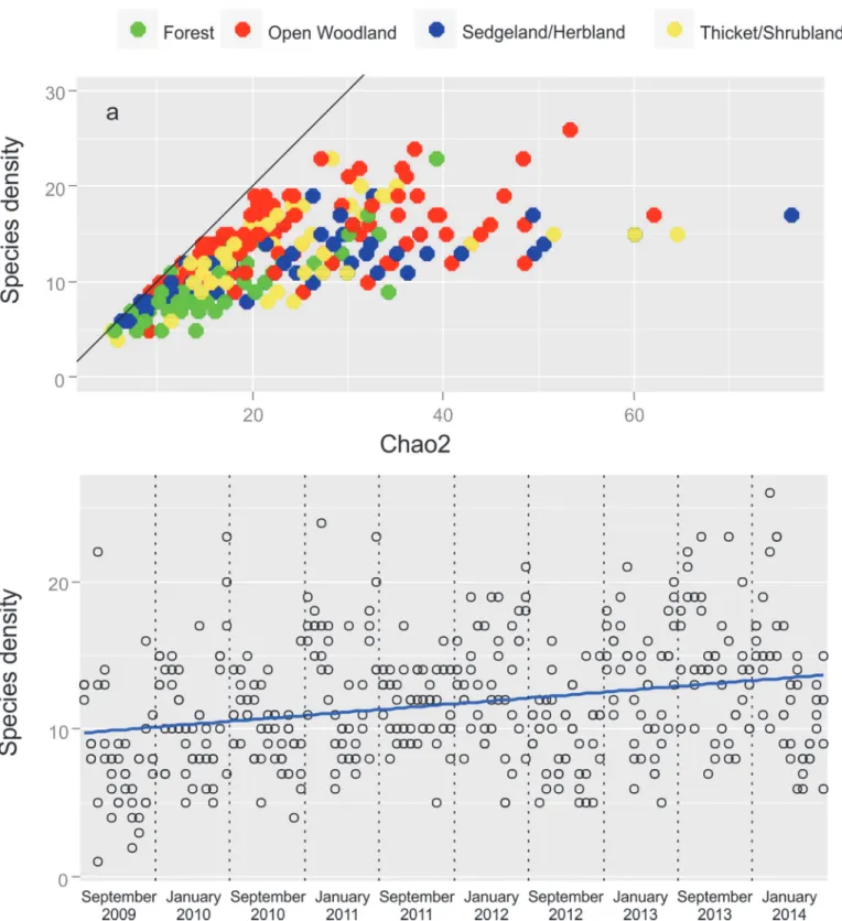
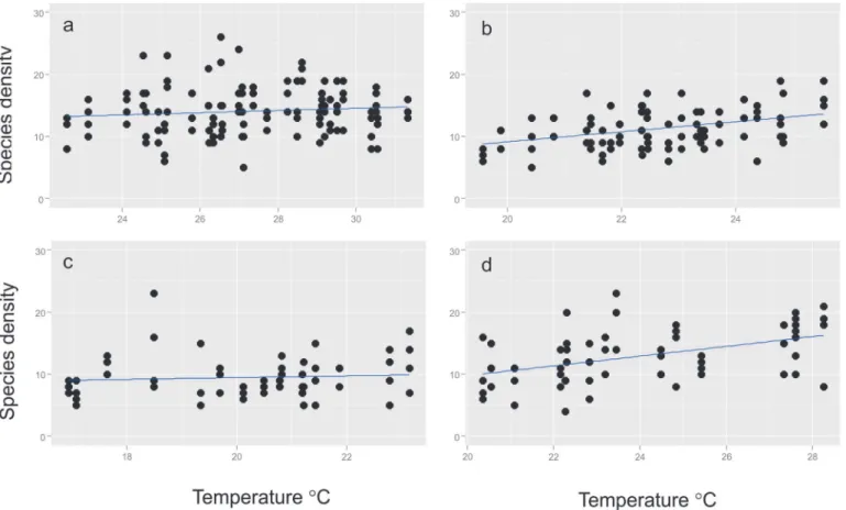
A total of 86502 ants comprised of 130 species in 38 genera and six subfamilies were collected. Sample coverage for the whole survey varied from 0.98–0.99 for a site while the mean coverage was 0.82 ± 0.005 (SE) for replicates during a sampling occasion. Species densities observed in a replicate averaged at 15 species with the highest richness observed in the open woodlands fol-lowed by the thicket/bushland of the lower southern elevations and sedgeland/herblands of the higher elevations, while forest sites had the lowest observed species densities (Fig. 1). Scatter-plots suggest that there is positive relationship between the average temperature during the month of the survey and the number of species observed (Fig. 2A—D). This pattern is the most evident for the thicket/shrubland and sedgeland/herbland habitats (Fig. 2C and D).
Drivers and correlates
The best model of species density retained average monthly temperature during the month of the survey, mid-domain effect, Soil-PC2, Soil-PC 3 and Soil-PC 4 as drivers and correlates (Table 1). The mid-domain effect’s estimate was highly significant (p<0.001) and positive
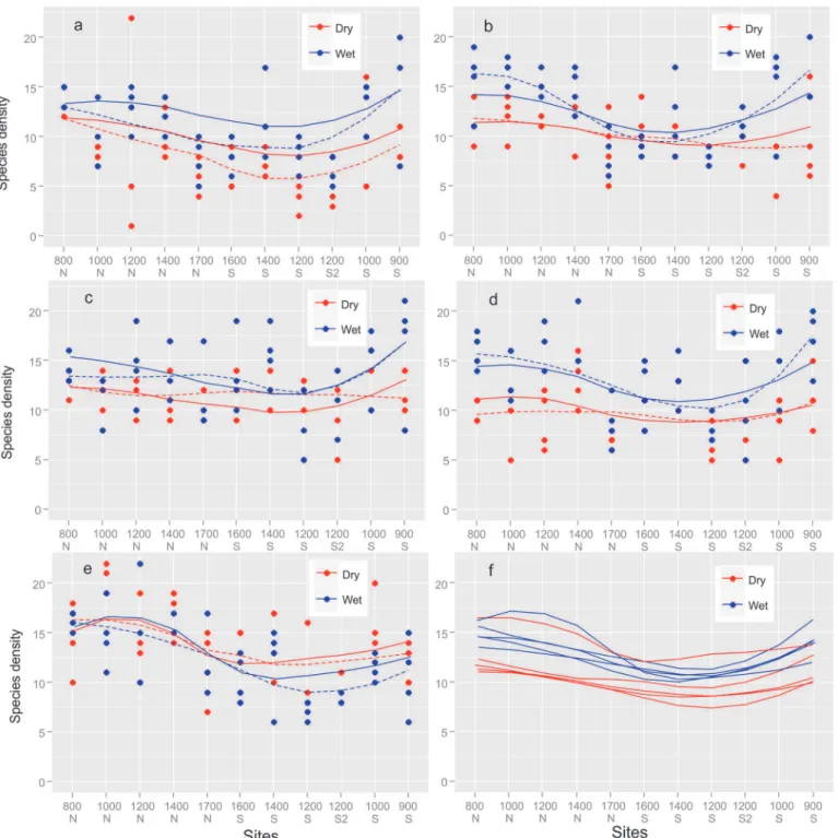
(Table 1). Average monthly temperature stood central to model performance and also performed the best when include as the only predictor in the model (Table 1). Average monthly temperature during the month of the survey also resembled the general form of ant richness patterns across the mountain (S2 Fig.). The best model had a marginal R2 of 0.33 while temperature alone ex-plained 22% of the variation. Temperature’s estimate was positive (0.1 ± 0.02) suggesting that species density increases with increasing temperature. The model describes a pattern that is con-sistently higher along the lower elevations of the southern aspect, lower in the forests and summit and hump-shaped or unchanged on the northern aspect (Fig. 3). Sites of the open woodlands on the northern aspect generally had the highest observed and predicted species richness.
Spatio-temporal covariates
Species density was higher during the wet seasons (Table 2) but there was an exception to this rule in the 2013/2014 sampling season when some sites on the southern aspect recorded higher species densities during the dry season than during the wet season (Fig. 3).The interaction of el-evation with season was negative and significantly so for the wet season. This points to a more pronounced decrease in species density with elevation. There has also been a significant annual increase in species densities over the period of the study (Table 2). Seven of the 31 spatial eigen-vectors (PCNM’s) were retained in the best model and their spatial structure is shown in
S9 Fig.These seven variables represents spatial structuring of ant species density patterns from the largest to the smallest spatial scale.
Analysis of model residuals
Spatio-temporal variables explained a small amount of variation in the residuals of the best driver model, R2m = 0.04, and suggest that there were no spatio-temporal pattern in the resid-uals of the best driver model and that all the variation is explained by temperature and mid-domain effect.
Seasonal variation in species density
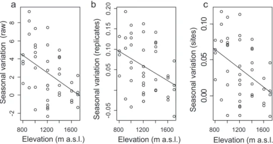
Seasonal variation in species density decreased significantly (b =−0.5–2, df = 42, p = 0.002)
with increased elevation even when the size of total species in replicates (b =−0.9–4, df = 42,
p = 0.001) and sites (b =−0. 9–4, df = 42, p = 0.003) or elevational bands were accounted for
Fig 1. Scatterplots of Species Density Collected at 11 sites.a) Scatterplots of observed species densities and Chao 2 estimates of species richness at replicates in the four habitat types along the transect and b) a scatterplots of species densities collected at the 11 sites as a function of the chronological order of surveys.
Fig 2. Scatterplots of Observed Species Density for Vegetation Types.Scatterplots of observed species densities against mean monthly temperatures recorded during the survey month when samples were collected in the a) open woodland, b) forests, c) sedgland/herbland, and d) thicket and shrubland.
doi:10.1371/journal.pone.0122035.g002
Table 1. Model AIC values, marginal and conditional R2for generalized linear mixed models of all drivers, correlates, spatio-temporal and the residuals of the best driver model.
Drivers
ΔAIC (next best)
Worst model
R2m R2c
Best Model 1450 (Average Temperature + Mid-domain + Soil-PC2 + Soil-PC3 + Soil-PC4) 1452 1463.7 0.33 0.38 Average
Temperature
1497.073 0.22 0.32
Mid-domain 1484.767 0.16 0.37
Soil-PC2 1540.136 0.06 0.27
Soil-PC3 1544.527 0.03 0.27
Soil-PC4 1547.546 0.005 0.27
Spatio-temporal
ΔAIC (next best)
Worst model
R2 m R2c
Best model 1489.437 (Elevation:Season+Year + Season + PCNM2 + PCNM3 + PCNM11 + PCNM13 + PCNM14 + PCNM17 + PCNM25)
1490 0.32 0.32
Year 1532.8 0.06 0.3
Season 1529.6 0.05 0.3
PCNM2 1537 0.08 0.26
Residuals of drivers model 0.04 0.52
Discussion
The most widely accepted pattern of richness along altitudinal gradients is the decline in rich-ness with increased elevation [55] although there has been growing support of richness peaking
Fig 3. Species Density different Sampling Season.Species density for different sampling events (10 surveys) across the elevational sites in the Soutpansberg mountain range (2009–2014) predicted from the model, red lines (dry season) September survey and black lines (wet season) January surveys and also for all years (ten in total) combined. Also a plot for species density against all 10 surveys for all elevational sites from northern aspect to southern slope overtime (September 2009—January 2014), similarly top lines, red line = dry season and black lines = wet season.
at mid-elevation [21,23,31,33,34,56,57]. Richness patterns along this transect are more com-plex with diversity peaking at mid-elevation on the northern slope of the mountain, decreasing at higher elevations [35,36,58,59] followed by a small intermediate peak towards mid-eleva-tion before reaching a peak at the lowest elevamid-eleva-tion of the southern slope, seeFig. 3F. The pat-terns remained constant throughout the study period.
Ant species density was mostly higher during the wet seasons. This is not surprising as ants are most active and abundant during this period (summer rainfall periods) in southern Africa [60]. The reversal of this trend during the 2013/2014 sampling season, when species densities were higher during the dry season, point to the considerable heterogeneity and variability ob-served in this savannah biome compared to the grassland biome in Southern Africa where wet seasons were consistently more diverse than dry seasons and could explain why models in our study explained less variation than models for ant diversity along elevations in grassland [23]. After controlling for the size of species pools (Fig. 4), the seasonal variation in species density still decreased with elevation, strengthening support for the impact of elevation on seasonal ef-fects [23]. Thus an increased richness was not the result of dispersal from the regional species pool but caused by decreased activity levels of ant colonies during cold and resource poor peri-ods (dry season). These conditions have a disproportionately higher impact on lower elevation species. These taxa are often less tolerant of colder temperatures experienced during the dryer seasons. Many of the predatory specialist, several of which were restricted to lower elevations e. g. ponerinae ants [61] were also only active during the wet season when prey availability peak-ed. Ant species density showed a significant increase over the period of the study (Fig. 1B).
Table 2. Estimates of significant terms in spatio-temporal and driver-correlate models of species densities observed over the period of the study.
Spatio-temporal
Term Estimates
Year 0.04±0.015*
Dry Season$Wet Season 0.4±0.04*
Elevation: Wet Season −0.0004±0.9 × 10⁻⁴*
Elevation: Dry Season −0.0001±0.9 × 10⁻⁴
PCNM2 0.0001±0.1 × 10⁻⁴***
PCNM3 −0.00004±0.1 × 10⁻⁴*
PCNM11 −0.00007±0.3 × 10⁻⁴*
PCNM13 0.0001±0.4 × 10⁻⁴
**
PCNM14 −0.00007±0.3 × 10⁻⁴**
PCNM17 0.00009±0.4 × 10⁻⁴*
PCNM25 0.0006±0.3 × 10⁻⁴
. Drivers and correlates
Mid-domain 0.12±0.02***
Monthly Average Temperature 0.1±0.02***
Soil-PC2 0.48±0.14***
Soil-PC3 −0.26±0.15.
Soil-PC4 0.26±0.14.
.,<0.01;
*,<0.05
**,<0.01
***,<0.001
The mid-domain effect played a prominent role in explaining variation in species density. Evidence for the importance of mid-domain effect has been found in other studies Dunn et al. [42] but support also exists for the contrary [22,62]. Sanders [21] in a regional elevational gra-dient study, reported on the importance of geometric constraints in explaining ant richness variation where the mid-domain effect together with available area explained 90%, 99% and 57% in Colorado, Nevada and Utah respectively. In contrast, a study in southern Appalan-chians of leaf-litter ants along an altitudinal gradient found no support for geometric con-straints models [22]. Kaspari, Ward [63] also found no support for these models at a
continental scale in North America. While Bishop, Robertson [23], although not directly test-ing for these models, argued that it is unlikely that neutral models are responsible for drivtest-ing patterns across their study area and pointed to the importance of temperature and area in ex-plaining diversity patterns observed. Our results highlight the importance of geometric con-straints and not area in explaining variation in richness.
There was a significant positive association between species density and percentage clay in the soil (Soil-PC2). Percentage clay negatively affected the dominance levels of dominant ants in the Kruger National Park [64] and distribution of Anoplolepis cf. custodiens in the Ceder-berg [11]. The abundance of the dominant ant Messor andrei, in North Californian grasslands, was negatively associated with percentage clay levels [65]. While it was positively related with the occurrence of more common ant species, Acropyga fuhrmanni in Ecuador [66]. In our study high percentage clay of the soil was associated with high species density and corresponds with Ramon, Barragan [67] observation that clay contribute to high species richness in Ecua-dorian Andean forests. Although Delsinne, Roisin [68] found no relationship between soil tex-ture and alpha diversity, their study further suggest the indirect effect of soil [66] on ant diversity through its impacts on plants e.g. excess salt in the soil negatively affect ant diversity through its effect on plant diversity.
At a larger and regional scale, Braschler, Chown [44] observed a unimodal relationship be-tween ant richness and NDVI with a peak at average productivity in sites of the Fynbos biome. The smaller scale of this study might explain why energy failed to have an effect [69]. NDVI
Fig 4. Seasonal Variation and Elevation.Relationship between seasonal variation in species density and elevation on both aspects of the mountain for a) raw species density, b) as proportion of total species observed in a replicate over the period of the study, c) and proportion of the total species observed at a site (elevational band).
might also be a poor proxy of available energy in this study. Particularly for the forests and hab-itats with considerable canopy cover where very little of this biomass will be available for epige-al ants.
Studies along an arid elevational transect stressed the importance of temperature where in combination with precipitation explained 80% of ant species variation [32]. Temperature con-strains ant foraging activities as it restricts their foraging times of the day [70]. It is also widely accepted as a principal factor that determines distribution and activities [71] and there is a growing evidence that low temperature is a primary stress that controls patterns in ants as well as community structure [72,73]. In contrast a study in Indonesian cacao plantations by Wiel-goss, Tscharntke [74] observed a negative correlation between temperature and ant species richness due to the presence of aggressive dominant Dolichoderinae ant species in the study area. Complex environments also have an influence on temperature indirectly, where open habitats tend to have high temperatures compared to closed/complex environment [72].
Similar to our study, complex habitats and low temperatures at higher elevations of Serra do Cipó [73] sampled less ants species. Soil temperatures in the thickets/shrubland and sedgeland/ herbland habitats were a better predictor of species density than the open woodlands and for-est. Thermal ranges in the forests are small (S3 Fig.(12S and 12S2)) and might act as a filter for a small subset of cold tolerant species. In contrast, open woodlands are characterised by consid-erable variation in micro-climates over very small scales. The two iButtons per site might there-fore not capture the varied thermal regimes of this habitat and fail to capture some of the variation in observed species density.
In conclusion, we found that geometric constraints were the most important driver of spe-cies density patterns followed by temperature while soil characteristics played a minor role. En-ergy, habitat structure and area failed to explain significant amounts of variation while spatio-temporal predictors were accounted for by the best model of drivers. In contrast to our sister transect in the Drakensberg mountains [23], we’ve observed an increase in species density over time. Similar to their study, seasonal variation in species density decreased with elevation. There was a significant decrease in richness with elevation during the wet season while this de-crease was not significant during the dry season. The strength of patterns therefore varied with season and elevation.
Supporting Information
S1 Table. Soil Properties.Soil properties of all 44 replicates along Soutpansberg transect. (PDF)
S2 Table. UTM Coordinates of Replicates.UTM coordinates of replicates as well as dummy variables that were included to reduce the threshold value and reduce the smallest scale that can be perceived.
(PDF)
S1 Fig. Site and soil properties Bioplot.Site and soil properties biplot of Principal Compo-nent Analysis. Red arrows indicate soil properties and black labels indicate replicates. (TIF)
S2 Fig. Boxplot of soil temperature.Boxplot of soil temperature at each site over the period of the study.
S3 Fig. Boxplot of Soil Temperature Monthly_a.Boxplot of soil temperatures at sites during the months when ants were sampled.
(TIF)
S4 Fig. Boxplot of Soil Temperature Monthly_b.Boxplot of soil temperatures at sites during the months when ants were sampled.
(TIF)
S5 Fig. Vertical Vegetation Structure.Vertical vegetation structure of all 44 replicates (aver-aged over the period of the study) along Soutpansberg transect.
(TIF)
S6 Fig. Horizontal Vegetation Structure.Horizontal vegetation structure of all 44 replicates (averaged over the period of the study) along Soutpansberg transect.
(TIF)
S7 Fig. Boxplot of NDVI.Boxplot of NDVI at each site over the period of the study. (TIF)
S8 Fig. UTM for 44 Replicates.UTM coordinates of 44 replicates along transect as well as the four dummy variables included in the Principal Coordinate Analysis of Neighbourhood Matri-ces. Inset is the minimum spanning tree used to calculate the maximum distance required to connect all replicates.
(TIF)
S9 Fig. Representation of Significant.Representation of significant eigenvectors in geographical space.
(TIF)
Acknowledgments
This research was funded by the DST-NRF, Centre of Excellence for Invasion Biology. Special thanks to Alan Andersen for verifying ant identifications. Norbert Hahn provided valuable input into the initial design of the transect. We are grateful to Ian Gaigher (Lajuma), Steven Fick (Koedoesvlei) and Dave Dewsnap (Goro) for providing access to their farms. Oldrich van Schalkwyk is thanked for weather data. Several volunteers from the University of Venda and Lajuma are thanked for their assistance in the field. The manuscript benefited from the inputs of two anonymous reviewers.
Author Contributions
Conceived and designed the experiments: TCM SHF. Performed the experiments: TCM SHF. Analyzed the data: TCM SHF. Contributed reagents/materials/analysis tools: TCM SHF. Wrote the paper: TCM SHF.
References
1. Laliberte´ E, Paquette A, Legendre P, Bouchard A. Assessing the scale-specific importance of niches and other spatial processes on beta diversity: a case study from a temperate forest. Oecologia. 2009; 159: 377–88. doi:10.1007/s00442-008-1214-8PMID:19018575
2. Bestelmeyer BT, Miller JR, Wiens JA. Applying species diversity theory to land management. Ecol Appl. 2003; 13: 1750–61.
3. Rohde K. Latitudinal gradient in species diversity: the search for the primary cause. Oikos 1992; 65: 514–27.
5. Pimm SL, Brown JH. Domains of Diversity. Science. 2004; 304: 831–3. PMID:15131295
6. Willig MR, Kaufman DM, Stevens GC. Latitudinal gradients of biodiversity: patterns, process, scale, and synthesis. Annu. Rev. Ecol. Evol. Syst. 2003; 34: 273–309.
7. Colwell RK, Lees DC. The mid-domain effect: geometric constraints on the geography of species rich-ness. Trends Ecol Evol. 2000; 15:70–6. PMID:10652559
8. Rosenzweig ML. Species diversity in space and time. New York, NY: Cambridge University Press; 1995.
9. Kattan GH, Franco P. Bird diversity along elevational gradients in the Andes of Colombia: area and mass effects. Global Ecol Biogeogr. 2004; 13: 451–8.
10. Strivastava DS, Lawton JH. Why more productive sites have more species: an experimental test of the-ory using tree-hole communities. Am. Nat. 1998; 152: 510–29. doi:10.1086/286187PMID:18811361
11. Botes A, McGeoch MA, Robertson HG, Van Niekerk A, Davids HP, Chown SL. Ants, altitude and change in the northern Cape Floristic Region. J Biogeogr. 2006; 33: 71–90.
12. Lyons SK, Willig MR. Species richness, latitude, and scale-sensitivity. Ecology. 2002; 83: 47–58. 13. McCain CM. Could temperature and water availability drive elevational species richness patterns? A
global case study of bats. J. Biogeogr. 2007b; 16: 1–13.
14. Rahbek C. The relationship among area, elevation, and regional species richness in Neotropical birds. Am. Nat. 1997; 149: 875–902. PMID:18811253
15. Cowling RM, Samways MJ. Predicting global patterns of endemic plant species. Biodiversity Letters. 1995; 2: 127–31.
16. Ellison AM. Macroecology of Mangroves: Large-large patterns and process in tropical Coastal forest Trees. Trees. 2002; 16: 181–94.
17. Lobo JM. Species diversity and composition of dung beetle (Coleoptera: Scarabaeoidea) assemblages in North America. Can Entomol. 2000; 132: 307–21.
18. Cerdar X, Retana J, Cros S. Thermal disruption Mediterranean of transitive hierarchies ant communi-ties. J Anim Ecol. 1997; 66: 363–74.
19. Colwell RK, Rangel TF. A stochastic, evolutionary model for range shifts and richness on tropical eleva-tional gradients under Quaternary glacial cycles. Phil. Trans. R. Soc. B. 2010; 365: 3695–707. doi:10. 1098/rstb.2010.0293PMID:20980317
20. Crous CJ, Samways MJ, Pryke JS. Grasshopper assemblage response to surface rockiness in Afro-montane grasslands. Insect Cons Divers. 2014; 7: 185–94.
21. Sanders NJ. Elevational gradients in ant species richness: area, geometry, and Rapoport's Rule. Eco-graphy. 2002; 25: 25–32.
22. Sanders NJ, Lessard J, Fitzpatrick MC, Dunn RR. Temperature, but not productivity or geometry, pre-dicts elevational diversity gradients in ants across spatial grains. Global Ecol Biogeogr. 2007; 16: 640–
9.
23. Bishop TR, Robertson MP, van Rensburg BJ, Parr CL. Elevation–diversity patterns through space and time: ant communities of the Maloti-Drakensberg Mountains of southern Africa. J Biogeogr. 2014; 41: 2256–68.
24. Sanders NJ, Moss J, Wagner D. Patterns of ant species richness along elevational gradients in an arid ecosystem. Global Ecol Biogeogr. 2003; 12: 93–102.
25. Hahn N. Endemic flora of the Soutpansberg. M.S.c Thesis, University of KwaZulu-Natal. 2002. Avail-able:http://www.soutpansberg.com/endemic_flora/pdf/endemic_flora_soutpansberg.pdf
26. Berger K, Crafford JE, Gaigher I, Gaigher MJ, Hahn N, Macdonald I. A first synthesis of the environ-mental, biological & cultural assets of the Soutpansberg. Louis Trichardt: Leach Printers & Signs CC; 2003.
27. Jocqué R. A new candidate for a Gondwanaland distribution in Zodariidae (Araneae): Australutica in Af-rica. Zookeys. 2008; 1: 59–66.
28. Kirchhof S, Kramer M, Linden J, Richter K. The reptile species assemblage of the Soutpansberg (Lim-popo Province, South Africa) and its characteristics. Salamandra. 2010; 46: 147–66.
29. Hahn N. Floristic diversity of the Soutpansberg, Limpopo Province, South Africa. PhD Thesis, Universi-ty of Pretoria; 2006.
30. Leal IR, Wirth R, Tabarelli M. The Multiple Impacts of Leaf-Cutting Ants and Their Novel Ecological Role in Human-Modified Neotropical Forests. Biotropica. 2014; 46: 516–28.
32. Sanders NJ, Moss J, Wagner D. Patterns of ant species richness along elevational gradients in an arid ecosystem. Global Ecol Biogeogr. 2003; 12: 93–102.
33. Sabu TK, Vineesh PJ, Vinod KV. Diversity of forest litter-inhabiting ants along elevations in the Waya-nad region of the Western Ghats. J Insect Sci. 2008; 8: 1536–2442.
34. Chaladze G. Climate-based model of spatial pattern of the species richness of ants in Georgia. J Insect Conserv. 2012; 16: 791–800.
35. Olson DM. The distribution of leaf litter invertebrates along a Neotropical altitudinal gradient. J. trop. ecol. 1994; 10: 29–150.
36. Robertson HG. Comparison of the leaf litter ant communities on woodlands, lowland forests and mon-tane forests of north-eastern Tanzania. Biodivers Conserv. 2002; 11: 167–52.
37. de Juan S, Hewitt J. Spatial and temporal variability in species richness in a temperate intertidal com-munity. Ecography. 2014; 37: 183–90.
38. Beck J, Altermatt F, Hagmann R, Lang S. Seasonality in the altitude–diversity pattern of Alpine moths. Basic Appl Ecol. 2010; 11: 714–22.
39. Munyai TC, Foord SH. Ants on a mountain: spatial, environmental and habitat associations along an al-titudinal transect in a centre of endemism. J Insect Conserv. 2012; 16: 677–95.
40. Foord SH, Gelebe V, Prendini L. Effects of aspect and altitude on scorpion diversity along an environ-mental gradient in the Soutpansberg, South Africa. J Arid Environ. 2015; 113: 114–20.
41. Abensperg-Traun M, Steven D. The effects of pitfall trap diameter on ant species richness (Hymenop-tera: Formicidae) and species composition of the catch in a semi-arid eucalypt woodland. J Ecol. 1995; 20: 282–7.
42. Adis J. Problems of interpreting arthropod sampling with pitfall traps. Zool Anz. 1979; 202: 177–84. 43. Clarke A, Gaston KJ. Climate, energy, and diversity. Proc. R. Soc. B. 2006; 273: 2257–66. PMID:
16928626
44. Braschler B, Chown SL, Gaston KJ. The Fynbos and Succulent Karoo Biomes Do Not Have Exception-al LocException-al Ant Richness. PLoS ONE. 2012; 7: e31463. doi:10.1371/journal.pone.0031463PMID:
22396733
45. Colwell RK. RangeModel: a Monte Carlo simulation tool for assessing geometric constraints on species richness. Version 5.—User's guide and application published at<http://viceroy.eeb.uconn.edu/ RangeModel>. 2006.
46. Dunn RR, Colwell RK, Nilsson C. The river domain: why are there more species halfway up the river? Ecography. 2006; 29: 251–9.
47. Borcard D, Legendre P, Avois-Jacquet C, Tuomisto H. Dissecting the Spatial Structure of Ecological Data at Multiple Scales. Ecology. 2004; 85: 1826–32.
48. R Development Core Team. R: A Langauge and Environment for Statistical Computing. In: Computing RFfS, editor. Vienna, Austria 2013.
49. Paknia O, Pfeiffer M. Niche-based processes and temporal variation of environment drive beta diversity of ants (Hymenoptera: Formicidae) in dryland ecosystems of Iran. Myrmecol. News. 2014; 20: 15–23. 50. Borcard D, Legendre P. All-scale spatial analysis of ecological data by means of principal coordinates
of neighbour matrices. Ecol Model. 2002; 152: 51–68.
51. Chao A, Jost L. Coverage-based rarefaction and extrapolation: standardizing samples by complete-ness rather than size. Ecology. 2012; 93: 2533–47. PMID:23431585
52. Del Toro I. Diversity of Eastern North American Ant Communities along Environmental Gradients. PLoS ONE. 2013; 8: e67973. doi:10.1371/journal.pone.0067973PMID:23874479
53. Nakagawa S, Schielzeth H. A general and simple method for obtaining R2 from generalized liner mixed models. Methods Ecol Evol. 2013; 4: 133–42.
54. Fleishman E, Austin GA, Weiss AD. An empirical test of rapoport's rule: elevational gradients in mon-tane butterfly communities. Ecology. 1998; 79: 2482–93.
55. Stevens GC. The elevational gradient in altitudinal range: An extension of Rapoport's latitudinal Rule to altitude. Am Nat. 1992; 140: 893–911. doi:10.1086/285447PMID:19426029
56. Rahbek C. The elevational gradient of species richness: a uniform pattern? Ecography. 1995; 18: 200–
5.
57. Fisher BL. Ant diversity patterns along an elevational gradient in the Reserve Special d’Anjanaharibe Sud and on the western Masoala Peninsula, Madagascar. Fieldiana Zoology. 1998; 90: 39–67. 58. Collins NM. The distribution of soil macrofauna on the West Ridge of Gunung (Mount) Mulu, Sarawak.
59. Atkin L, Proctor J. Invertebrates in the litter and soil on volcan Barva, Costa Rica. J. Trop. Ecol. 1988; 4: 307–10.
60. Parr CL, Robertson HG, Biggs HC, Chown SL. Response of African savanna ants to long-term fire re-gimes. J Appl Ecol. 2004; 41: 630–42.
61. Munyai TC, Foord SH. An inventory of epigeal ants of the western Soutpansberg mountain range, South Africa. Koedoe. In press.
62. Kerr JT, Perring M, Currie DJ. The missing Madagascan mid-domain effect. Ecol Lett. 2006; 9: 149–59. PMID:16958880
63. Kaspari K, Ward PS, Yuan M. Energy gradients and the geographic distribution of local ant diversity. Oecologia. 2004; 140: 407–13. PMID:15179582
64. Parr CL. Dominant ants can control assemblage species richness in a South African savanna. J Anim Ecol. 2008; 77: 1191–8. doi:10.1111/j.1365-2656.2008.01450.xPMID:18637854
65. Boulton AM, Davis KF, Ward PF. Species richness, abundance, and composition of ground-dwelling ants in northern california grasslands: role of plants, soil, and grazing. Environ. Entomol. 2005; 34: 96–
104.
66. Jacquemina J, Drouet T, Delsinnea T, Roisinb Y, Leponcea M. Soil properties only weakly affect sub-terranean ant distribution at small spatial scales. Appl. soil Ecol. 2012; 62: 163–9.
67. Ramon G, Barragan A, Donoso DA. Can clay banks increase the local ant species richness of a mon-tane forest? Métodos en Ecología y Sistemática. 2013; 8: 37–58.
68. Delsinne T, Roisin Y, Herbauts J, Leponce M. Ant diversity along a wide rainfall gradient in the Para-guayan dry Chaco. J Arid Environ. 2010; 74: 1149–55.
69. Kaspari M, O’Donnell S, Kercher JR. Energy, Density, and Constraints to Species Richness: Ant As-semblages along a Productivity Gradient. Am. Nat. 2000; 155: 281–91.
70. Jayatilaka P, Narendra A, Reid D, Cooper J, Zeil J. Different effects of temperature on foraging activity schedules in sympatric Myrmicia ants. J. Exp. Biol. 2011; 214: 2730–8. doi:10.1242/jeb.053710PMID:
21795570
71. Hölldobler B, Wilson EO. The ants. Massachusetts: Harvard University Press; 1990.
72. Andersen AN. Global ecology of rainforest ants: functional groups in relation to environmental stress and disturbacne. In: Agosti D, Majer JD, Alonso LE, Schultz R, editors. Ants: standard methods for measuring and monitoring biodiversity. Washington D.C.: Smithsonian Insitution Press; 2000. p. 25–34.
73. Araújo L, Fernandes G. Altitudinal patterns in a tropical ant assemblage and variation in species rich-ness between habitats. Lundiana. 2003; 4: 103–9.