www.hydrol-earth-syst-sci.net/21/43/2017/ doi:10.5194/hess-21-43-2017
© Author(s) 2017. CC Attribution 3.0 License.
Processing and performance of topobathymetric lidar data
for geomorphometric and morphological classification
in a high-energy tidal environment
Mikkel Skovgaard Andersen1, Áron Gergely1, Zyad Al-Hamdani2, Frank Steinbacher3, Laurids Rolighed Larsen4, and Verner Brandbyge Ernstsen1
1Department of Geosciences and Natural Resource Management, University of Copenhagen, Copenhagen, Denmark 2Geological Survey of Denmark and Greenland, Copenhagen, Denmark
3Airborne Hydro Mapping GmbH, Innsbruck, Austria 4NIRAS, Allerød, Denmark
Correspondence to:Verner Brandbyge Ernstsen ([email protected])
Received: 5 January 2016 – Published in Hydrol. Earth Syst. Sci. Discuss.: 19 January 2016 Revised: 21 October 2016 – Accepted: 27 November 2016 – Published: 3 January 2017
Abstract. The transition zone between land and water is difficult to map with conventional geophysical systems due to shallow water depth and often challenging environmen-tal conditions. The emerging technology of airborne topo-bathymetric light detection and ranging (lidar) is capable of providing both topographic and bathymetric elevation infor-mation, using only a single green laser, resulting in a seam-less coverage of the land–water transition zone. However, there is no transparent and reproducible method for pro-cessing green topobathymetric lidar data into a digital ele-vation model (DEM). The general processing steps involve data filtering, water surface detection and refraction correc-tion. Specifically, the procedure of water surface detection and modelling, solely using green laser lidar data, has not previously been described in detail for tidal environments. The aim of this study was to fill this gap of knowledge by developing a step-by-step procedure for making a digital wa-ter surface model (DWSM) using the green laser lidar data. The detailed description of the processing procedure aug-ments its reliability, makes it user-friendly and repeatable. A DEM was obtained from the processed topobathymetric lidar data collected in spring 2014 from the Knudedyb tidal inlet system in the Danish Wadden Sea. The vertical accu-racy of the lidar data is determined to±8 cm at a 95 %
con-fidence level, and the horizontal accuracy is determined as the mean error to ±10 cm. The lidar technique is found
ca-pable of detecting features with a size of less than 1 m2. The
derived high-resolution DEM was applied for detection and classification of geomorphometric and morphological fea-tures within the natural environment of the study area. Ini-tially, the bathymetric position index (BPI) and the slope of the DEM were used to make a continuous classification of the geomorphometry. Subsequently, stage (or elevation in re-lation to tidal range) and a combination of statistical neigh-bourhood analyses (moving average and standard deviation) with varying window sizes, combined with the DEM slope, were used to classify the study area into six specific types of morphological features (i.e. subtidal channel, intertidal flat, intertidal creek, linear bar, swash bar and beach dune). The developed classification method is adapted and applied to a specific case, but it can also be implemented in other cases and environments.
1 Introduction
sailing, swimming, hiking, diving and surfing. In addition to human exploitation, climate change also poses a future threat with a predicted rising sea level and increasing storm inten-sity and frequency, expected to cause erosion and flooding in the coastal zone (Mousavi et al., 2011). All these pressures and different interests underpin the societal need for high-resolution mapping, monitoring and sustainable management in the coastal zone.
Historically, the transition zones between land and water have been difficult or even impossible to map and investi-gate in high spatial resolution due to the difficulties in col-lecting data in these challenging, high-energy environments. The airborne near-infrared (NIR) light detection and rang-ing (lidar) is a technique often used for measurrang-ing high-resolution topography; however, the NIR laser is incapable of measuring bathymetry due to the absorption and reflec-tion of the laser light at the water surface. Tradireflec-tionally, high-resolution bathymetry is measured with a multibeam echosounder (MBES) system mounted on a vessel, but it does not cover the bathymetry in the shallow water due to the vessel draft limitation.
NIR lidar and MBES are applied in different environ-ments; however, the data are very similar and the processed high-resolution topography/bathymetry is often captured, vi-sualized and analysed in a digital elevation model (DEM). The processed DEM may be applied for various purposes, e.g. for geomorphological mapping. Previous studies clas-sifying morphology in either terrestrial or marine environ-ments have been performed numerous times (Al-Hamdani et al., 2008; Cavalli and Marchi, 2008; Hogg et al., 2016; Höfle and Rutzinger, 2011; Ismail et al., 2015; Kaskela et al., 2012; Lecours et al., 2016; Sacchetti et al., 2011). These classi-fication studies generally focus on either the marine or the terrestrial environment and do not cover the fine-scale mor-phology in the shallow water, due to the challenging envi-ronmental conditions. To overcome this impediment, a new generation of airborne green topobathymetric lidar that en-ables high-resolution measurements of both topography and shallow bathymetry has been introduced (Guenther, 1985; Jensen, 2009; Pe’eri and Long, 2011). The potential of merg-ing morphological classifications of marine and terrestrial environments enables a holistic approach for managing the coastal zone.
The raw topobathymetric lidar measurements are spatially visualized as points in a point cloud, with each point contain-ing information of its location and elevation. The point cloud must be piped through a series of steps before it can be vi-sualized as a DEM. Most of the processing steps required to process raw topobathymetric lidar data into a DEM are sim-ilar to the processing steps of topographic lidar data (Huis-ing and Gomes Pereira, 1998). However, additional process-ing steps are required for topobathymetric lidar data due to the refraction of the laser beam at the water surface. All submerged lidar points have to be corrected for refraction; therefore, the water depth must be known for each point.
This sets a requirement for making a digital water surface model (DWSM), before the refraction correction can be per-formed.
Often, the water surface is detected and modelled from si-multaneous collection of green and NIR lidar measurements, where the green laser reflects from the seabed and the NIR laser reflects from the air–water interface, and the NIR laser data are then used to detect and model the water surface (Al-louis et al., 2010; Collin et al., 2008; Guenther, 2007; Parker and Sinclair, 2012). The use of NIR lidar data for water sur-face detection has been applied in several studies. For in-stance, Höfle et al. (2009) proposed a method for mapping water surfaces based on the geometrical and intensity infor-mation from NIR lidar data. Su and Gibeaut (2009) classified water points from NIR lidar based on point density, inten-sity and elevation. They identified the shoreline based on the large sudden decrease in NIR lidar intensity values when go-ing from land to water. Brzank et al. (2008) used the same three variables (point density, intensity and elevation) in a supervised fuzzy classification to detect the water surface in a section of the Wadden Sea. Another study in the Wadden Sea by Schmidt et al. (2012) used a range of geometric char-acteristics as well as intensity values to classify water points from NIR lidar data.
The capability of NIR lidar data for detecting the wa-ter surface is thus well documented. However, deriving all the information from a single green lidar dataset would be a more effective solution for water surface and seabed de-tection, with respect to the financial expenses and the diffi-culties of storing and handling often very large amounts of data. However, there is no definitive method for making a DWSM from green topobathymetric lidar data. For this pur-pose, the Austrian lidar company RIEGL have developed a software, RiHYDRO (RIEGL, 2015), in which it is possible to model the water surface in a two-step approach: (1) clas-sification of water surface points based on areas with two layers (water surface and seabed) and extending the classifi-cation to the entire water body, and (2) generation of a ge-ometric gridded DWSM for each flight swath based on the classified water surface points. However, RiHYDRO is com-mercial software, and thus the algorithms, which form the basis of the classification and water surface modelling, are not publicly available. Other software packages, such as Hy-droFusion (Optech, 2013) and LiDAR Survey Studio (Leica, 2015), also proclaim to have incorporated methods for the entire data processing workflow, but the algorithms in these software packages are also closed and cannot be accessed by public users.
eleva-tion, because the green water surface returns are actually a mix of returns from the air–water interface and from volume backscatter returns, and they are generally found as a cloud of points below the water surface. Mandlburger et al. (2013) addressed the second issue by comparing the water surface points of NIR and green lidar data, and they concluded that it is possible to derive the water surface elevation from the green lidar data with sub-decimetre vertical precision rela-tive to a reference water surface derived by the NIR lidar data. However, their work addressed only the determination of the water surface elevation without going into detail on the actual procedure of generating a DWSM. An approach for modelling the water surface from green lidar data was presented by Mandlburger et al. (2015), who did their study in a riverine environment with only few return signals from the water surface. Their method was based on manual es-timates of the water level in a series of river cross sections, after which interpolation between the cross sections filled out the gaps with no water surface points to derive a continuous water surface model.
The aim of this study was to investigate the potential of im-proving the procedure of processing green lidar data and gen-erating DEMs in tidal environments, and of improving the classification of morphological units in such environments. More specifically, the objectives were
1. to develop a robust, repeatable and user-friendly pro-cessing procedure of raw green lidar data for generating high-resolution DEMs in land–water transition zones; 2. to quantify the accuracy and precision of the green lidar
data based on object detection; and
3. to automatically classify morphological units based on geomorphometric analyses of the generated DEM. The investigations were based on studies undertaken in a sec-tion of the Knudedyb tidal inlet system in the Danish Wadden Sea.
2 Study area
The Knudedyb tidal inlet system is located between the bar-rier islands of Fanø and Mandø in the Danish Wadden Sea (Fig. 1a). The tidal inlet system is a natural environment without larger influence from human activity. The tides in the area are semi-diurnal, with a mean tidal range of 1.6 m, and the tidal prism is on the order of 175×106m3(Pedersen and
Bartholdy, 2006). The main channel is approximately 1 km wide and with an average water depth of approximately 15 m (Lefebvre et al., 2013).
The study site is an elongated 3.2 km2(0.85 km×4 km) section of the Knudedyb tidal inlet system (Fig. 1b). The section is located perpendicular to the main channel and stretches across both topography and bathymetry. The study site extends northward into an area on Fanø with dispersed
cottages (Fig. 1c). The most prominent morphological fea-tures within the study site include beach dunes (Fig. 1d), small mounds (Fig. 1e), swash bars (Fig. 1f and g) and linear bars (Fig. 1h).
3 Methods
3.1 Topobathymetric lidar
The topobathymetric lidar technique is based on continuous measurements of the distance between an airplane and the ground/seabed. The distance (or range) is calculated by half the travel time of a laser beam going from the airplane to the surface of the earth and back to the airplane. The wave-length of the laser beam is in the green spectrum, usually 532 nm, since this wavelength is found to attenuate the least in the water column, resulting in the largest penetration depth of the laser (Jensen, 2009). In literature, topobathymetric li-dar data are sometimes referred to as either bathymetric lili-dar or airborne lidar bathymetry. These are different terms with the same meaning, and in this paper, topobathymetric lidar is preferred, since it describes the system’s ability to simulta-neously measure bathymetry as well as topography.
A single laser beam may encounter many targets of vary-ing nature on its way from the airplane and back again, and different processes are influencing the laser beam propaga-tion through air and water. First, the laser beam may be re-flected by targets in the air, such as birds or dust particles, and these can show up as lidar points in the space between the air-plane and the surface. When encountering water, the speed of the laser decreases from 3×10⁸to, e.g. 2.25×10⁸m s−1in
10◦C freshwater or, e.g. 2.24×10⁸m s−1in 10◦C saltwater of 30 PSU (Millard and Seaver, 1990).
The changing speed of the laser beam also affects the di-rection of the laser beam when penetrating the water surface with an angle different from nadir (Fig. 2) (Guenther, 2007; Jensen, 2009). The laser beam will be refracted according to Snell’s law:
sinαair sinαwater
= cair
cwater
=nwater
nair , (1)
whereαairis the incidence angle of the laser beam relative to the normal vector of the water surface andαwateris the refrac-tion angle in water.nwaterandnair are the refractive indices of water and air, respectively (Mandlburger et al., 2013).
Figure 1. (a)Overview of the study area location in the Danish Wadden Sea (22 April 2014 satellite image, Landsat 8).(b)The study site in the Knudedyb tidal inlet system (30 May 2014 Orthophoto, AHM). Panel(c)shows cottages in the dunes on Fanø;(d)beach dunes on Fanø; (e)patch ofSpartina townsendii(common cord grass);(f)–(g)swash bars;(h)linear bar;(i)validation site 1 with a cement block on land,
used for accuracy and precision assessment (19 April 2014 orthophoto, AHM);(j)validation site 2 with a steel frame in Ribe Vesterå River, used for precision assessment (19 April 2014 orthophoto, AHM).
The returned signal is represented as a distribution of en-ergy over time, also called the “full-waveform” distribution (Alexander, 2010; Chauve et al., 2007; Mallet and Bretar, 2009). The peaks in the full-waveform distribution are de-tected as individual targets encountered by the propagating laser beam. If the laser hits two targets with a small
et al., 2009). The dead zone is a clear limitation to the lidar measurements, which is an important parameter to consider in very shallow water, such as intertidal environments. 3.2 Surveys and instruments
Lidar data and orthophotos were collected by Airborne Hydro Mapping GmbH (AHM) during two surveys on 19 April 2014 and 30 May 2014.
On 19 April 2014, the quality of the lidar data was vali-dated at two sites along Ribe Vesterå River (Fig. 1i and j):
– Validation site 1, with a 2.50×1.25×0.80 m cement
block, is located on land next to the mouth of Ribe Vesterå River (Fig. 1i). The block was covered by seven swaths retaining 227 lidar points from the block surface, which were used for assessing the accuracy and preci-sion of the lidar data.
– Validation site 2, with a 0.92×0.92×0.30 m steel
frame, is located in the Ribe Vesterå River, its top sit-uated just below the water surface (Fig. 1j). The frame was covered by four swaths retaining 46 lidar points from the surface of the frame, which were used for pre-cision assessment, and for testing the feature detection capability of the lidar system. According to the Inter-national Hydrographic Organization survey standards, cubic features of at least 1 m2 should be detectable in special order areas, which are areas with very shallow water as in the study site (IHO, 2008).
Ground control points (GCPs) were measured for the four corners of the block with an accuracy better than 2 cm using a Trimble R8 RTK GPS. Measurements were repeated three times and averaged to minimize errors caused by measure-ment uncertainties. GCPs were also collected for the frame; however, during the lidar survey the frame experienced an unforeseen intervention by local fishermen using the frame as fishing platform. Therefore, the frame was only used to assess the deviation between the lidar points (the precision) and not to assess the deviation between the lidar points and the GCPs (the accuracy).
On 30 May 2014, the study site was covered by 11 swaths, which were used for generating the DWSM and DEM. The overflight was carried out during low tide, and the water level was measured to −1 m DVR90 at Grådyb Barre,
approxi-mately 20 km NW of the study site.
The weather conditions were similar during the two sur-veys, with sunny conditions, average wind velocities of 7– 8 m s−1(DMI, 2014) and significant wave heights, measured west of Fanø at 15 m water, of approximately 0.5 m com-ing from NW (DCA, 2014). However, the waves in the less-exposed Knudedyb tidal inlet were observed in the 30 May lidar point cloud to be 0.2–0.3 m, which can be explained by the location of the study site in lee of the western-most inter-tidal flats and the ebb-inter-tidal delta. The wave heights in the rest
Figure 2.Conceptual sketch of the laser beam propagation and re-turn signals. The beam refracts upon entering the water body, and it diverges as it propagates through the water column. Return signals are produced in the air, at the water surface, in the water column and at the seabed. The lidar instrument has limited capability in very shallow water (the dead zone in the figure) because the successive peaks from the water surface and the seabed are not individually separated in time and amplitude. Only the largest peak, which is from the seabed, is detected.
of the study site (flood channel and intertidal ponds) were in the scale of sub-decimetres. There were no waves at valida-tion site 2 during the 19 April lidar survey.
Lidar data were collected with a RIEGL VQ-820-G topo-bathymetric airborne laser scanner in both surveys (RIEGL, 2014). The scanner was characterized by emitting green laser pulses with 532 nm wavelength and 1 ns pulse width. It had a very high laser pulse repetition rate of up to 520 000 Hz. The flying altitude was 400 m, which, combined with a beam divergence of 1 mrad, created a laser beam footprint of 40 cm diameter at the ground. The high repetition rate and nar-row footprint made it well suited to capture fine-scale land-forms (Doneus et al., 2013; Mandlburger et al., 2011). An arc-shaped scan pattern results in a swath width of approx-imately 400 m, while maintaining an almost constant 20◦ (±1◦) incidence angle of the laser beam when penetrating
the water surface (Niemeyer and Soergel, 2013). The typical water depth penetration of the laser scanner is claimed by the manufacturer to be one Secchi disc depth (RIEGL, 2014).
3.3 Processing raw topobathymetric lidar data into a gridded DEM
The essential processing steps, which are standard procedure when processing topobathymetric lidar data, were followed to produce a DEM in the study area. These steps included
1. determination of flight trajectory;
2. boresight calibration: calculating internal scanner cali-bration;
3. collecting topobathymetric lidar data;
4. swath alignment based on boresight calibration: the bias between individual swaths was minimized;
5. filtering: the raw data contained noise located both above and below ground, which needed to be filtered from the point cloud;
6. water surface detection: a DWSM had to be established in order to correct for refraction in the following step; 7. refraction correction: all the points below the water
sur-face in the DWSM were corrected for the refraction of the laser beam; and
8. point cloud to DEM: the points were transformed into a gridded elevation model representing the real world ter-rain in the study area, including cottages and vegetation on Fanø in the northern part.
Step 1 and 2 were performed prior to the lidar survey. The different instruments (lidar, inertial measurement unit (IMU) and GPS) were integrated spatially by measuring their po-sition relative to each other, when mounted on the airplane, and temporally by calibrating their time stamps.
Step 3 was the actual lidar survey and step 4 was the initial processing step after the lidar survey. The bias be-tween the swaths was minimized in the software RiPRO-CESS (RIEGL LMS) by automatically searching for planes in each swath and then matching the planes between the swaths.
Steps 5–8 represent the processing of the point cloud into a DEM. The methods involved in these steps are the main focus in this study and they are described in detail in the following subsections. Each swath was pulled individually through the processing workflow to account for the continually changing water level in the study area due to tides. The broad term DEM is used, rather than the more specific terms “digital terrain model” (DTM) or “digital surface model” (DSM), be-cause the generated model includes natural terrain in the tidal environment, which is the main focus area in this study, as well as vegetation and cottages on Fanø.
3.3.1 Filtering
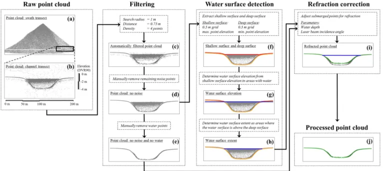
The raw lidar data contained noise in the air column origi-nating from the laser being scattered by birds, clouds, dust and other particles, and noise was also appearing below the ground/seabed (Fig. 3a and b). This noise had to be filtered before further processing. The filtering process involved both automatic and manual filtering.
The automatic filtering was carried out in Hydro-Vish (AHM) with the tool “Remove flaw echoes” (Fig. 3c). The filtering tool was controlled by three variable parame-ters: search radius, distance and density. The search radius parameter specified the radius of a sphere in which the dis-tance and density filters were utilized. The disdis-tance param-eter rejected a point, if it was too far from any other point within the sphere. The density parameter specified the lower limit of points within the sphere. The automatic filter iter-ated through all the points in the point cloud. The settings for the automatic filtering were based on a sensitivity analy-sis of three fragments of the lidar data, and the settings were selected so that a minimum of valid points were removed by the automatic filter. The settings were the following: search radius=1 m, distance=0.75 m and density=4 points.
The automatic filter could not remove two layers of noise points closely above and below ground, but on the other hand, more widely dispersed points in the deeper bathymetry were removed. To account for this, the point cloud went through manual filtering in Fledermaus (QPS) software, where the remaining noise points were rejected and the valid bathymetric points were accepted (Fig. 3d).
The filtered point cloud (with water points) was used in the following step to detect the water surface. Meanwhile, a copy of the data was undergoing additional manual filtering, removing all the water points (Fig. 3e). After this final fil-tering step, there were only points representing topography, bathymetry, vegetation and man-made structures left in the dataset.
3.3.2 Water surface detection
The water surface detection was based on determining the water surface elevation and the water surface extent, thereby producing a DWSM. The water surface elevation was deter-mined based on the water surface points, and the extent was determined by extrapolating the water surface until it inter-sected the surface of the topography. Two assumptions were made in the production of the DWSM:
simi-Figure 3.Workflow for processing the lidar point cloud. Panel(a)shows point cloud from a single swath with points ranging from−100 to
300 m elevation;(b)zoom-in on a cross section of the flood channel with elevation exaggerated×15 for visualization purpose;(c)–(e)method
for filtering the point cloud;(f)–(h)method for detecting a water surface (blue) based on the extraction of a shallow surface (red) and a deep surface (orange);(i)correction for the effect of refraction on all the submerged points;(j)processed point cloud.
lar fit through the lidar points along the flood channel showed a slope of 0.156×10⁻³ (0.009◦). The
maxi-mum wave heights observed in the main channel were 20–30 cm. Based on the moderate slope of the water sur-face and relatively low wave height, the water sursur-face was assumed to be flat. This assumption is deemed er-ror prone, but at the time of this study, it was our best estimate.
2. The study area contained water bodies with two differ-ent water levels: one represdiffer-ented the water level in the main channel and the other represented the water level in the flood channel. This was also a simplification, as the tidal flat contained small ponds with potentially dif-ferent water levels. However, almost all of these ponds contained no lidar points of the water surface, which means that the water depth in the ponds must have been within the limitation of the dead zone. Therefore, it was impossible to detect individual water surfaces in the ponds.
A series of processing steps was performed to produce the DWSM. The first step was to extract a shallow surface and a deep surface from the filtered point cloud (with water points) in Fledermaus (Fig. 3f). Both surfaces consisted of 0.5 m×0.5 m cells, and the elevation of each cell was equal
to the highest point within the cell (shallow surface) and the lowest point within the cell (deep surface), respectively. The shallow surface should then display the topography along with the water surface, whereas the deep surface should
dis-play the topography and the seabed (as long as the seabed was detected by the laser). It is worth noting that the extrac-tion of the shallow surface and the deep surface had nothing to do with the final DEM, as they were merely intermediate steps performed for the water surface detection.
The following steps were focused on the shallow surface to determine the elevation of the water surface (Fig. 3g). First, the shallow surface was down sampled to a surface with a cell size of 2 m×2 m, and the new cells were populated with the
maximum elevation of the input cells. The down sampling was done for smoothing the water surface and thereby elimi-nating most of the outliers. The exact cell size of 2 m×2 m,
as well as populating them with the maximum value, was chosen based on the work by Mandlburger et al. (2013). They compared water surface detection capability between green lidar data, collected with the same RIEGL-VQ-820-G laser scanner, and NIR lidar data, which were assumed to capture the true water surface. They found that the green lidar gener-ally underestimated the water surface elevation, but that re-liable results were achieved by increasing the cell size and only taking the top 1–5 % of water points into account. Ac-cording to their work, it was assumed that placing the water surface on the highest points in 2 m cells provided a good estimate of the true water level. However, based on their re-sults it could be expected that the water surface elevation in this case would be underestimated on the order of 2–4 cm.
cells within each area was calculated, and these values con-stituted the elevation of the water surfaces in the main chan-nel and in the flood chanchan-nel, respectively. Two horizontal wa-ter surfaces were created in the flood channel and the main channel with a cell size of 0.5 m×0.5 m and cell values equal
to the calculated water surface elevations. The high spatial resolution of 0.5 m cells was chosen to produce a detailed DWSM along the edges of the land–water transition.
Finally, the extent of the water surfaces was determined by subtracting the deep surface cell elevations from the wa-ter surface elevation and discarding all cells with resulting negative values (Fig. 3h), together forming the DWSM. 3.3.3 Refraction correction
The refraction correction of all the points below the DWSM was calculated in HydroVish (AHM). The input parameters were the filtered point cloud (without water points), the de-rived DWSM and the trajectory data of the airplane. The refraction correction was calculated automatically for each point based on the water depth, the incident angle of the laser beam and the refracted angle according to Snell’s law (Eq. 1 and Fig. 3i).
3.3.4 Point cloud to DEM
After iterating through the processes of filtering, water sur-face detection and refraction correction for all the individual swaths, the lidar points of all swaths were combined. The transformation from point cloud into a DEM was performed with ArcGIS (ESRI) software. The DEM was created as a raster surface with a cell size of 0.5 m×0.5 m, and each cell
was attributed the average elevation of the points within the cell boundaries. It was chosen to make the resolution of the DEM lower than the laser beam footprint size (i.e. 40 cm), due to the inaccuracies arising from attributing smaller cells with measured elevation values spanning across a larger area. Furthermore, the 0.5 m cell size was chosen to get as high resolution as possible without making any significant inter-polation between the measurements. In this way, each cell represented actually measured elevations instead of interpo-lated values. However, there were still very few gaps of in-dividual cells with no data in the resulting raster surface in areas with relatively low point density. Despite the general intention of avoiding interpolation, it was chosen to populate these cells with interpolated values to obtain a full cover-age DEM (except for the bathymetric parts beyond the max-imum laser penetration depth). The arguments for interpola-tion were that (1) the interpolated cells were scattered and represented only 1.7 % of all the cells, (2) they were found primarily on the tidal flat where the slope is generally less than 1◦, meaning that the elevation difference from one cell to a neighbouring cell is usually less than 1 cm, and (3) the general point density in most of the study area was so high that the loss of information by lowering the DEM resolution
would represent a larger sacrifice than interpolating a few scattered cells. The interpolation was performed by assign-ing the average value of all neighbourassign-ing cells to the empty cells. The final DEM was thereby fully covering the topogra-phy, and the bathymetry was covered down to a depth equal to the maximum laser penetration depth.
3.4 Accuracy and precision of the topobathymetric lidar data
The term accuracy refers to the difference between a point coordinate (in this case, a lidar point) compared to its “true” coordinate measured with higher accuracy, e.g. by a total sta-tion or a differential GPS, while the term precision refers to the difference between successive point coordinates com-pared to their mean value, i.e. the repeatability of the mea-surements (Graham, 2012; Jensen, 2009; RIEGL, 2014).
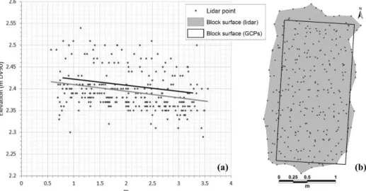
Two “best-fit planes” based on the lidar points on the block and the frame surfaces were established with the “Curve fit-ting tool” in MATLAB (MathWorks). We propose the use of these two planes to give an indication of the relative precision of the lidar measurements.
Another best-fit plane was established based on the block GPS measurements, and this plane was regarded as the true block surface for assessment of the accuracy of the lidar measurements. The established planes were described by the polynomial equation
z(x, y)=a+bx+cy, (2) wherex,yandzare coordinates anda,bandcare constants. Insertingx andy coordinates for the lidar surface points in Eq. (2) led to a result of the corresponding elevation (z) as projected on the fitted plane. The difference between the el-evation of the lidar point and the corresponding elel-evation on the fitted plane was used as a measure of the vertical ac-curacy (for the GCP-fitted plane of the block) and the ver-tical precision (for the lidar-point-fitted plane of the block and the frame). Statistical measures of the standard devia-tion (σ), mean absolute error (EMA) and root mean square error (ERMS) were calculated by
σ=
s P
zi−zplane2
n−1 (3)
EMA=
P
zi−zplane
n (4)
ERMS=
s P
zi−zplane2
n , (5)
Standards Part 3: National Standard for Spatial Data Accu-racy” (NSSDA) (FGDC, 1998):
Cl95 %=ERMS·1.96. (6)
The horizontal accuracy was determined as the horizontal mean absolute error (EMA,xy) based on the horizontal dis-tances between the block corners, measured with RTK GPS, and the best approximation of the block corners derived from the lidar points of the block surface. The minimum dis-tance between a block corner and the perimeter of the li-dar points was regarded as the best approximation. Hereafter, EMA,xywas calculated as the average of the four corners. 3.5 Geomorphometric and morphological
classifications
The processed DEM was applied in two classification anal-yses: first, a geomorphometric classification and then a mor-phological classification. Both were based on the DEM and derivatives of the DEM, but they were differentiated by the resulting classification classes, which showed (1) surface ge-ometry and (2) surface morphology. The analysis mode, as defined by Pike et al. (2009), was “general” in the geo-morphometric classification where the surface geometry was continuously classified within the study site, while being “specific” in the morphological classification where discrete morphological units were classified. The northern part of the study site with cottages on Fanø was excluded in the classifi-cation analyses, as the objective of this work was to classify the natural terrain (geomorphometry and morphology) in the high-energy and dynamic tidal environment.
3.5.1 Geomorphometric classification analysis
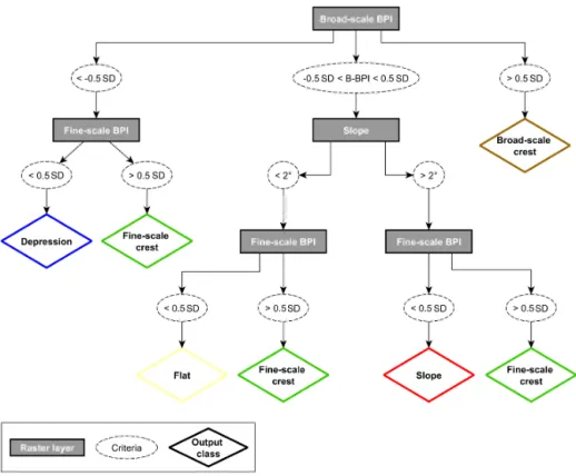
The benthic terrain modeler (BTM) tool (Wright et al., 2005) was used for the geomorphometric classification. The tool is an extension to ArcGIS Spatial Analyst, originally used for analysing MBES data (Diesing et al., 2009; Lundblad et al., 2006; Rinehart et al., 2004). The BTM classification tool uses fine- and broad-scale bathymetric position indexes (BPIs) (Verfaillie et al., 2007) in a multiple-scale terrain analysis to classify fine- and broad-scale geometrical features. The BPIs are measures of the elevation of a cell compared to the ele-vation of the surrounding cells within the determined scale (radius) size. Positive BPI values indicate a higher elevation than the neighbouring cells and negative BPI values indicate a lower elevation than the neighbouring cells. For instance, a BPI value of 100 corresponds to 1 SD (standard deviation) and a value of −100 corresponds to −1 SD of the cell
el-evation compared to the elel-evation of the surrounding cells within the determined scale size. BPI values close to zero are derived from flat areas or from constant slopes.
The elevation values of each cell in the DEM were exag-gerated by a factor of 10 before the classification to enable the BTM to detect the shapes of the terrain. The fine and
broad scales were determined based on the BPI results for different radius sizes. The best results were obtained from a broad-scale BPI of 100 m radius and a fine-scale BPI of 10 m radius, based on visual inspection. The fine- and broad-scale BPIs were used together with the slope of the actual DEM (not the exaggerated) to classify the investigated area into the geomorphometric classes: fine-scale crests, broad-scale crests, depressions, slopes and flats (Fig. 4). The clas-sification classes were decided based on previous studies us-ing the BTM classification tool with success (Diesus-ing et al., 2009; Lundblad et al., 2006). The thresholds for the fine- and broad-scale BPIs were in previous studies often defined as 1 SD (Lundblad et al., 2006; Verfaillie et al., 2007); how-ever, thresholds of 0.5 SD have also previously been applied (Kaskela et al., 2012). We used a low threshold of 0.5 SD due to the generally very gentle variations in the terrain ge-ometry of the tidal inlet system. We defined the threshold between slopes and flats as 2◦. This definition was a compro-mise between detecting as many slopes as possible but avoid-ing too many “false slopes” beavoid-ing detected along the swath edges, which seemed to be a consequence of lower precision at the outer beams of the swath, as well as differences be-tween overlapping swaths.
3.5.2 Morphological classification analysis
A morphological classification was developed for delineat-ing actual morphological features in the study area. The clas-sification was built partly on different neighbourhood analy-ses and slopes derived from the DEM and partly on the lo-cal tidal range. Broad-slo-cale crests from the geomorphometric classification were also incorporated in the analysis. Figure 5 describes the steps performed in ArcGIS, which led to the classification of six morphological classes: swash bars, linear bars, beach dunes, intertidal flats, intertidal creeks and sub-tidal channels. All the criteria for defining a particular mor-phological class had to be fulfilled for a cell to be classified into that class. Cells that did not meet the criteria to be classi-fied into any of the morphological classes were assigned the class “unclassified”.
A total of 33 years of continuous measurements of the wa-ter level at Havneby on Rømø, 25 km south of the study area, showed a mean low water level of−0.94 m (DVR90) and
a mean high water of 0.94 m (DVR90) (Klagenberg et al., 2008). Although the tidal range in Knudedyb was probably slightly different, it was the best estimate for the study site. Therefore, these water levels were used to separate between the supratidal, intertidal and subtidal zones.
Subtidal channels were defined as everything below the mean low water, which was−0.94 m. A “smooth DEM” was
created, in which each cell of the original DEM was as-signed the average elevation value of its surrounding cells in a window size of 100 m×100 m (actually 199×199 cells,
i.e. 99.5 m×99.5 m). The result was subtracted from the
Figure 4.Classification decision tree, showing how the geomorphometric classification was conducted in the benthic terrain model tool.
Table 1.Vertical accuracy and precision of the lidar point measurements, in terms of minimum error (Emin), maximum error (Emax), standard deviation (σ), mean absolute error (EMA), root mean square error (ERMS) and the 95 % confidence level (Cl95 %).
Accuracy/ Object Best-fit # points Emin Emax σ EMA ERMS Cl95 %
precision plane No. (cm) (cm) (cm) (cm) (cm) (cm)
Accuracy Cement block GCPs 227 0.01 12.1 4.1 3.5 ±4.1 ±8.1
Precision Cement block Point cloud 227 0.04 12.9 3.9 2.8 ±3.9 ±7.6
Precision Steel frame Point cloud 46 0.02 5.5 2.0 1.6 ±1.9 ±3.8
which made it possible to extract information about the de-viation of the cells in the DEM compared to its surrounding cells. The principle is similar to the BPI, and again the pur-pose was to locate cells with a higher/lower elevation than its surrounding cells. Positive values were higher cells and negative values were lower cells. Certain thresholds were found suitable for classifying beach dunes (>0.8 m) and in-tertidal creeks (<−0.3 m). These two classes were further
classified into their respective tidal zones (supratidal and in-tertidal) based on the elevation. Intertidal flats were classi-fied by low slope values (<1◦) of a down-sampled 2 m DEM (each down-sampled cell was assigned the mean value of its 4×4 original cells). Moreover, to be classified as a flat, the
ECM had to be within±10 cm to avoid any incorrect
inter-tidal flat classification of flat crests on top of bars or flat bottoms inside creeks or channels. The BTM classification class “broad-scale crests” was used as an input, since it was found to capture bar features. However, the thresholds used in the BTM classification resulted in capturing features larger than bars in the broad-scale crests class. To distinguish be-tween bars and larger features, the standard deviation of each DEM cell in a moving window size of 250 m×250 m
(actu-ally 249×249 cells, i.e. 124.5 m×124.5 m) was calculated.
A suitable threshold to distinguish between bars and larger features was 0.6 SD. Finally, swash bars and linear bars were identified by an area/perimeter ratio, based on the assump-tion that linear bars have a smaller ratio than swash bars due to the different shapes. Based on visual interpretation, a ratio of 4 was found to be a suitable threshold.
4 Results
4.1 Refraction correction and dead zone extent
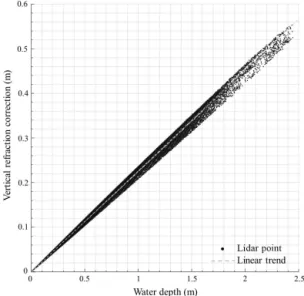
The vertical adjustment of the lidar points (zdiff) due to refraction correction is linearly correlated with the water depth (d) (Fig. 6). An empirical formula is derived for this relationship:
zdiff=0.227·d R2=0.997. (7)
A lidar point at 1 m water depth is vertically adjusted by ap-proximately 0.23 m (Fig. 6). The variations around the linear trend in Fig. 6 are due to changing incidence angles of the
Figure 6.Vertical adjustment of the refracted lidar points from the flood channel transect (see location in Fig. 1b).
laser beam that varies with the airplane attitude (roll, pitch and yaw).
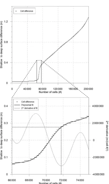
The vertical extent of the dead zone is approxi-mately 28 cm, determined by plotting the vertical difference between the shallowest and the deepest lidar point within 0.5 m cells – i.e. between the shallow surface and the deep surface (Fig. 7). The difference is manifested by an abrupt change at the dead zone, and the highest rate of change is shown to be at a water depth of approximately 28 cm.
4.2 Sub-decimetre accuracy and precision
The vertical root mean square error of the lidar data is
±4.1 cm, and the accuracy is ±8.1 cm with a 95 %
confi-dence level (Table 1 and Fig. 8a). The vertical precision of the lidar data with a 95 % confidence level is±3.8 cm for the
points on the frame and±7.6 cm for the points on the block
(Table 1).
Table 2.Lidar point spacing and density for all the 11 individual swaths, which covered the study area, and for the combined swaths.
Swath number 1 2 3 4 5 6 7 8 9 10 11 All
Point spacing (m) 0.30 0.30 0.36 0.31 0.36 0.32 0.37 0.29 0.35 0.36 0.28 0.20 Point density (pt. m−2) 10.8 10.8 7.8 10.2 7.5 9.6 7.2 11.7 8.0 7.8 12.7 19.6
Figure 7.Vertical difference between the shallowest and the deepest lidar point within 0.5 m grid cells in the land–water transition zone. The abrupt change is caused by the dead zone. The vertical extent of the dead zone is determined to approximately 28 cm, derived by the maximum rate of change of a polynomial fit through the points.
4.3 Point density and resolution
The average point density is 20 points per m2, which equals an average point spacing of 20 cm (Table 2). The point den-sity of the individual swaths varies between 7 and 13 points per m2, and the point density of the combined swaths in the study area varies between 0 and 216 points per m2, although densities above 50 points per m2are rare.
4.4 DEM and landforms
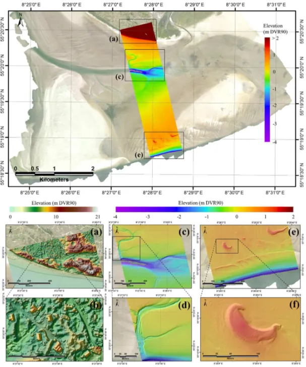
The elevations in the studied section of the Knudedyb tidal inlet system range from−4 m DVR90 in the deepest parts of
the flood channel and main channel to 21 m DVR90 on top of the beach dunes on Fanø (Fig. 9). Beach dunes and cottages of the village Sønderho are clearly visible in the northern part of the study site (Fig. 9a and b). The intertidal zones are gen-erally flat, while the most varying morphology is found in the area of the flood channel (Fig. 9c and d) and in the area close to the main channel (Fig. 9e and f). The flood chan-nel is approximately 200 m wide in the western part and it divides into two channels towards the east. The bathymetry of the channel bed is clearly captured by the lidar data in the eastern part and also in the western part down to−4 m
DVR90, which approximately equals a water depth of 3 m at the time of survey. An intertidal creek joins the flood chan-nel from the north (Fig. 9d). From the flood chanchan-nel towards south, the tidal flat is vaguely upward sloping, until it reaches two distinct swash bars, which are rising 0.9 m above the sur-rounding tidal flat, reaching a maximum elevation of 1.5 m DVR90 (Fig. 9e and f). Further south, the linear bars along the margin of the main channel are clearly captured in the DEM (Fig. 9e).
4.5 Geomorphometric and morphological classifications
Figure 8.Vertical and horizontal distribution of the lidar points describing the block surface and the actual block surface derived from GCPs. (a)lidar points (grey dots) compared to the GCP block surface (black line) for determining the vertical accuracy. The grey line shows the lidar block surface as a best linear fit through the points.(b)Block surface derived from the four GCP corner points and the block surface derived by the perimeter of the lidar points.
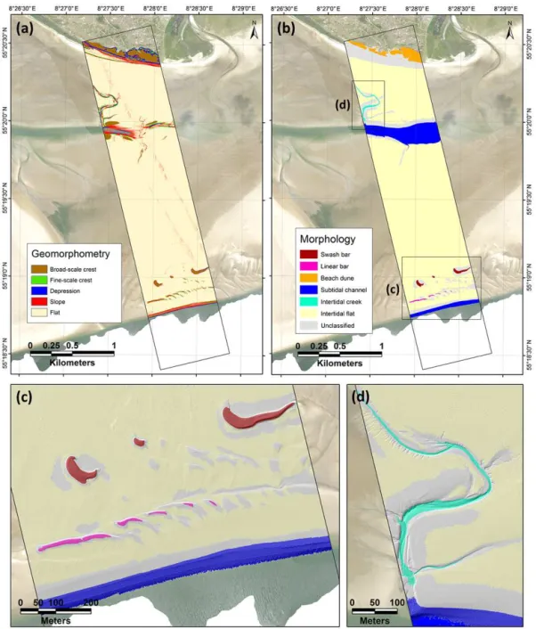
also found on Fanø in the northern part of the area, and most of these are classified as beach dunes in the morphological classification. The geomorphometric classification identifies more broad-scale crests along the banks of the flood channel; however, these are not real bar features but they are identified as crests due to the nearby flood channel and creeks resulting in a positive broad-scale BPI. In the morphological classi-fication, it is possible to distinguish between these and the actual bar features by looking at elevation deviations at an even broader scale than the broad-scale BPI. The intertidal creek in the northwestern part of the area is a mix of depres-sions, slopes and fine-scale crests in the geomorphometric classification, whereas it is relatively well defined and prop-erly delineated in the morphological classification (Fig. 10d). The geomorphometric classification identifies slopes along the banks of the main channel, flood channel and the intertidal creek, as well as in front of the beach dunes and along the edges of the swash bars and linear bars. The slopes seem particularly reliable at delineating the features in the in-tertidal zone, i.e. swash bars, linear bars and creeks. Depres-sions are primarily identified in the deepest detected parts of the main channel and in the flood channel, in the intertidal creek and in the beach dunes. Fine-scale crests are found in the geomorphometric classification in locations which are high compared to its near surroundings. They are primarily seen as parts of the linear bars close to the main channel, in the beach dunes on Fanø and along the banks of the intertidal creeks.
A few small circular mounds of approximately 5 m diame-ter with patches ofSpartina townsendii(common cord grass)
located on the intertidal flat are classified as fine-scale crests in the geomorphometric classification (Fig. 11). It clearly
shows the capability of capturing fine-scale features in the DEM and in the derived classification.
5 Discussion
5.1 Performance of the water surface detection method The water surface in topobathymetric lidar surveys are most often detected from NIR lidar data and are simultaneously collected along with the green lidar data (Collin et al., 2012; Guenther et al., 2000; Parker and Sinclair, 2012; Wang and Philpot, 2007). However, detecting the water surface and generating a DWSM based on the green lidar data alone pro-vides a potential to perform topobathymetric surveys with just one sensor, thus optimizing the survey costs as well as data handling and storage.
Figure 9.Topobathymetric DEM across the northern part of the Knudedyb tidal inlet system with close-up views of different detail level in specific areas. The northern supratidal part of the study area(a, b)includes beach dunes, vegetation and cottages; thus, the DEM can be regarded as a DSM in this specific section. In the subtidal and intertidal parts of the study area(c–f), the DEM reflects the natural terrain; thus, it can be regarded as a DTM. Panel(a)shows beach dunes, vegetation and cottages;(b)cottages;(c)flood channel;(d)intertidal creek; (e)swash bars, linear bars and bathymetry of the main channel;(f)swash bar. A hillshade is draped upon the close-up views for improved visualization of morphological features.
method for modelling the water surface; however, it was done in a fluvial environment and the water level was based on manual determinations of cross-sectional water levels. The water surface detection method in this study is thus new in combining the following properties: (1) it is only using green lidar data, (2) it is based on automatic water level determina-tion, (3) it is applied in a tidal environment (can be applied in
any coastal environment) and (4) it is transparent and repeat-able due to the detailed description of data processing steps given in the text.
Figure 10.Two classifications derived from topobathymetric lidar data:(a)geomorphometric classification and(b)morphological classi-fication. Panel(c)indicates zoom-in on the swash bars and linear bars close to the main channel in the morphological classification and (d)zoom-in on the intertidal creek in the morphological classification. A hillshade of the DEM is draped over(c)and(d).
surface is indeed a simplification of the real world, since the water surface in reality can be inclined, and it can be topped by waves.
5.2 Implications of the dead zone
The vertical extent of the dead zone is in this study deter-mined to approximately 28 cm (Fig. 7), which means that no return signal is detected from the water surface when the water depth is less than 28 cm. The implication of the dead
pond will result in −6 cm elevation error according to the
calculated refraction (Fig. 6).
5.3 Evaluation of the topobathymetric lidar data quality
The vertical accuracy of conventional topographic lidar data has previously been determined to±10–15 cm (Hladik and
Alber, 2012; Jensen, 2009; Klemas, 2013; Mallet and Bre-tar, 2009). Only few previous studies have focused on the accuracy of shallow water topobathymetric lidar data (Man-dlburger et al., 2015; Nayegandhi et al., 2009; Steinbacher et al., 2012). Nayegandhi et al. (2009) determined the vertical ERMS of lidar data in 0–2.5 m water depth to±10–14 cm,
which is above the±4.1 cmERMS found in this study (Ta-ble 1). Steinbacher et al. (2012) compared topobathymet-ric lidar data from a RIEGL VQ-820-G laser scanner with 70 ground-surveyed river cross sections serving as refer-ence, and found that the system’s error range was±5–10 cm,
which is comparable to the ±8.1 cm accuracy found in this
study. Mandlburger et al. (2015) compared ground-surveyed points from a river bed with the median of the four near-est 3-D neighbours in the lidar point cloud, and they found a standard deviation of 4.0 cm, which is almost equal to the
±4.1 cm standard deviation found in this study (Table 1). In
comparison with these previous findings of lidar accuracy, the assessment of the vertical accuracy in this study indicates a good quality of the lidar data.
Mapping the full coverage of tidal environments, such as the Wadden Sea, requires a combination of topobathymet-ric lidar to capture topography and shallow bathymetry and MBES to capture the deeper bathymetry. The two technolo-gies make it possible to produce seamless coverage of en-tire tidal basins; however, merging the two products raises the question whether the quality of the data from the two different sources is comparable. Comparing the lidar accu-racy with previous findings of accuaccu-racy derived from MBES systems indicates similar or slightly better accuracy from the MBES systems (Dix et al., 2012; Ernstsen et al., 2006). Dix et al. (2012) determined the vertical accuracy of MBES data by testing the system on different objects and in differ-ent environmdiffer-ents and found the verticalERMSto be±4 cm.
Furthermore, they tested a lidar system on the same objects and found a similar vertical ERMS of ±4 cm. The vertical
ERMS of ±4.1 cm found in this study is very close to both
the MBES accuracy and lidar accuracy determined by Dix et al. (2012). Another study by Ernstsen et al. (2006) de-termined the vertical precision of a high-resolution shallow-water MBES system based on seven measurements of a ship-wreck from a single survey carried out in similar settings as the present study, namely in the main tidal channel in the tidal inlet just north of the inlet investigated in this study. They found the vertical precision to be ±2 cm, which is
slightly better than the vertical precision of±3.8 cm (frame)
and±7.6 cm (block) found in this study. Overall, accuracy
and precision are within the scale of sub-decimetres for both topobathymetric lidar and MBES systems, which enables the mapping of tidal basins with full coverage and with compa-rable quality.
Due to technical and logistical reasons, the data validation and the actual survey were carried out on different days and in different locations. Based on this, it is a fair question to ask whether the determined quality actually represents the qual-ity of the data within the study site. Differences between the determined data quality at the validation sites and the data quality at the study site may arise from (1) different environ-mental conditions on the two surveying days and/or (2) dif-ferent environments at the validation sites compared to the study site.
The environmental conditions were similar on the two sur-veying days (as mentioned in Sect. 3.2), meaning that the different days are not affecting the representation of the data quality within the study site.
The environmental differences between validation site 2 and the study site include the presence of up to 0.2–0.3 m waves in the main channel next to the study site. The waves introduce a source of error, because the proposed water sur-face detection method is not modelling the waves. The pre-cision of the seabed points within the study site are therefore expected to be worse than the±3.8 cm precision determined
at validation site 2.
Figure 11.Vegetated mounds on the intertidal flat are clearly visible in the DEM and classified as fine-scale crests in the geomorphometric classification. To the right is an image of one of the mounds.
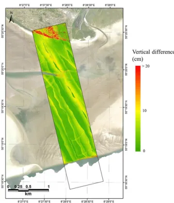
Figure 12.Vertical difference between the highest and the lowest lidar point within 0.5 m×0.5 m grid cells.
5.4 Spatial variations of topobathymetric lidar data quality
The quality of spatial datasets is often provided as single values, such as ±8.1 cm for the vertical accuracy in this
case, and then the determined value represents the accu-racy/precision of the whole dataset. However, in reality the value is only a measure of the local quality at the location where the assessment is conducted. The quality of the dataset varies spatially, and one way to illustrate this is to extract the maximum vertical difference between the lidar points of the processed point cloud within every 0.5 m×0.5 m cell
throughout the study site (Fig. 12). In flat areas, without mul-tiple return signals, this shows the spatially varying precision of the dataset. There are large differences on Fanø, which is expected due to vegetation causing multiple lidar returns from both the vegetation canopy and from the bare ground. In contrast, the differences on the very gently sloping, non-vegetated tidal flat are up to 10 cm, and there is no simple and natural reason for this variation. A range of factors contribute to the observed variations:
– The laser beam incidence angle is determined by a com-bination of the scan angle, the water surface angle and the terrain slope. The shape of the footprint is stretched with larger incidence angles, and this effect can cause pulse timing errors in the detected signal, which lead to a decreasing vertical accuracy (Baltsavias, 1999). The error associated with larger scan angles is generally causing the outer beams, toward the swath edges, to at-tain a lower accuracy (Guenther, 2007). This is a rea-son for the observed variations along the swath edges (Fig. 12). Terrain slopes have the same effect of decreas-ing the vertical accuracy due to the footprint stretch-ing. The measured elevation tends to be biased toward the shallowest point of the slope within the laser beam (Guenther, 2007). However, the influence of slope is not crucial in the Knudedyb tidal inlet system, since it is generally a very flat area.
– The water depth is a factor, since the accuracy and precision are expected to be lower as the laser beam penetrates deeper into the water column (Kunz et al., 1992). The laser beam footprint is diverging as it moves through the water column, resulting in a larger footprint on the seabed. The elevation of the detected point is thus derived from the measurement on a larger area on the seabed, which will decrease the vertical accuracy, as well as decrease the capability of detecting small objects. With this in mind, the higher precision at the frame compared to the block is opposite of what would be expected, since the frame is below water and the block is on land. In this case, other factors, such as over-lapping swaths and/or scan angle deviations, have more influence on the precision than the water depth. Also, it should be remembered that the frame surface was close to the water surface, and the effect of the water depth on the precision would most likely be more evident if it was located in deeper water.
Additional factors, beside the ones mentioned above, may influence the quality of lidar datasets. For instance, a dense vegetation cover of the seabed or breaking waves that makes the laser detection of the seabed almost impossible. However, these factors do not have a great influence in the studied part of the Knudedyb tidal inlet system, and thus they are not fur-ther elaborated.
5.5 Evaluation of the morphological classification The morphological classification presented in this study is based on the studied section of the Knudedyb tidal inlet sys-tem. The overall concept of using tidal range, slope and vari-ations of the elevation at different spatial scales proves to be a reliable method for delineating the morphological features in this tidal environment. The concept, however, can be ap-plied in other environments. The specific thresholds in the classification determined in this study may deviate in other areas. Morphological features of different sizes require steps of other spatial scales in the neighbourhood analyses to pro-duce a successful classification. In the future, the classifica-tion method will be improved by implementing an objective method for determining the scales, which can make it appli-cable in areas with different morphological characteristics. Such an objective scale determination method is presented by Ismail et al. (2015), who determined the scales based on the variance of the DEM at progressively larger window sizes. In this way, the sizes of the morphological features are deter-mining the scales for the classification.
5.6 Using topobathymetric lidar data to map
morphology in a highly dynamic tidal environment The study demonstrates the capability of green topobathy-metric lidar to resolve fine-scale features, while covering a broad-scale tidal inlet system. Collecting topobathymetric
li-dar data with a high point density of 20 points per m2on av-erage enables detailed seamless mapping of large tidal envi-ronments, and the lidar data have further proved to maintain a high accuracy. The combined characteristics of mapping with high resolution and high accuracy in a traditionally challeng-ing environment provide many potential applications, such as mapping for purposes of spatial planning and management, safety of navigation, nature conservation, or morphological classification, as demonstrated in this study. The developed lidar data processing method is tailored to a morphological analysis application. The best representation of the morphol-ogy is mapped by gridding the average value of the lidar points into a DEM with a 0.5×0.5 resolution. Other
appli-cations would require different gridding techniques. For in-stance, hydrographers, who are generally interested in map-ping for navigational safety, would use the shallowest point for gridding. However, the overall method for processing the point cloud can be used regardless of the application. Only the last and least-challenging/time-consuming step of grid-ding the point cloud into a DEM may vary depengrid-ding on the application.
Applying topobathymetric lidar data for morphological analyses in tidal environments enables a holistic approach of seamlessly merging marine and terrestrial morphologies in a single dataset. However, a combination of topobathymetric lidar and MBES data is required, in order to map the mor-phology of tidal environments in full coverage. The compa-rable quality and resolution of lidar and MBES data gives a potential to map broad-scale tidal environments, such as the Wadden Sea, in full coverage and with high resolution and high accuracy.
6 Conclusions
A method was developed for processing raw topobathymet-ric lidar data into a DEM with seamless coverage across the land–water transition zone. The method relies on basic prin-ciples, and the entire processing method is described with a high level of detail, which makes it transparent and easy to implement for future studies. Specifically, a new proce-dure was developed for water surface detection in a tidal environment utilizing automatic water level determination solely based on green lidar data. The water surface detection method presented in this work did not take into account the variation in wave heights and surface slopes, which therefore constitutes a challenge to be addressed in future studies.
The vertical accuracy of the lidar data was determined by object detection of a cement block on land to±8.1 cm with a
95 % confidence level. The vertical precision was determined at the cement block to±7.6 cm, and±3.8 cm at a steel frame
placed just below the water surface. The horizontal mean er-ror was determined at the block to±10.4 cm. Overall,
A seamless topobathymetric DEM was created in a 4 km×0.85 km section in the Knudedyb tidal inlet system.
An average point density of 20 points per m2made it possi-ble to create an elevation model of 0.5 m×0.5 m resolution
without significant interpolation. The DEM extended down to water depths of 3 m, which was determined as the max-imum penetration depth of the laser scanning system at the given environmental conditions. Measurements of suspended sediment concentration and organic matter content indicated that the penetration depth was limited by the amount of or-ganic matter rather than the amount of suspended sediment.
The vertical dead zone of the lidar data was determined to approximately 0–28 cm in the very shallow water.
The DEM was used as input in the benthic terrain modeler tool to classify the study area into five classes of geomor-phometry: broad-scale crests, fine-scale crests, depressions, slopes and flats. A morphological classification method was developed for classifying the area into six morphological classes: swash bars, linear bars, beach dunes, intertidal flats, intertidal creeks and subtidal channels. The morphologi-cal classification method was based on parameters of tidal range, terrain slope, a combination of various statistical neighbourhood analyses with varying window sizes and the area/perimeter ratio of morphological features. The concept can be applied in any coastal environment with knowledge of the tidal range and the input of a DEM; however, the thresholds may need adaptation, since they have been de-termined for the given study area. In the future, the classi-fication method should be improved by implementing an ob-jective method for determining thresholds, which makes it immediately applicable across different environments.
Overall, this study has demonstrated that airborne topo-bathymetric lidar is capable of seamless mapping across land–water transition zones even in environmentally chal-lenging coastal environments with high water column tur-bidity and continuously varying water levels due to tides. Furthermore, we have demonstrated the potential of topo-bathymetric lidar in combination with morphometric anal-yses for classification of morphological features present in coastal land–water transition zones.
7 Data availability
The raw topobathymetric lidar data and the processed DEM cannot be distributed; however, the data can be made avail-able by contacting the corresponding author.
Author contributions. Verner Brandbyge Ernstsen designed the
study within the research project “Process-based understanding and prediction of morphodynamics in a natural coastal system in re-sponse to climate change”. Frank Steinbacher and Laurids Ro-lighed Larsen collected the lidar data. Mikkel Skovgaard Ander-sen and Áron Gergely performed the groundtruthing fieldwork and processed the lidar and groundtruthing data. Mikkel Skovgaard
An-dersen, Zyad Al-Hamdani and Verner Brandbyge Ernstsen analysed and interpreted the data and drafted the paper, which was then edited by all co-authors.
Competing interests. The authors declare that they have no conflict of interest.
Acknowledgements. This work was funded by the Danish Council
for Independent Research – Natural Sciences through the project “Process-based understanding and prediction of morphodynamics in a natural coastal system in response to climate change” (Steno grant no. 10-081102) and by the Geocenter Denmark through the project “Closing the gap! – Coherent land–water environmental mapping (LAWA)” (grant no. 4-2015). We give thanks to QPS for providing the Fledermaus software suite. We thank the anonymous reviewers and the editor for comments and suggestions which improved the final version of the paper.
Edited by: A. Guadagnini
Reviewed by: three anonymous referees
References
Alexander, C.: Classification of Full-waveform Airborne Laser Scanning Data and Extraction of Attributes of Vegetation for To-pographic Mapping, PhD Thesis, University of Leicester, Leices-ter, 2010.
Al-Hamdani, Z., Alanen, U., Andersen, J. H., Bekkby, T., Bendtsen, J., Bergström, U., Buˇcas, M., Carlén, I., Dahl, K., and Daunys, D.: Baltic Sea marine landscapes and habitats-mapping and mod-eling, BALANCE Technical Summary Report, part 2/4, Geolog-ical Survey of Denmark and Greenland, Copenhagen, 2008. Allouis, T., Bailly, J. S., Pastol, Y., and Le Roux, C.: Comparison
of LiDAR waveform processing methods for very shallow water bathymetry using Raman, near-infrared and green signals, Earth Surf. Proc. Land., 35, 640–650, 2010.
Baltsavias, E. P.: Airborne laser scanning: basic relations and for-mulas, ISPRS J. Photogramm., 54, 199–214, 1999.
Brzank, A., Heipke, C., Goepfert, J., and Soergel, U.: Aspects of generating precise digital terrain models in the Wadden Sea from lidar–water classification and structure line extraction, ISPRS J. Photogramm., 63, 510–528, 2008.
Cavalli, M. and Marchi, L.: Characterisation of the surface mor-phology of an alpine alluvial fan using airborne LiDAR, Nat. Hazards Earth Syst. Sci., 8, 323–333, doi:10.5194/nhess-8-323-2008, 2008.
Chauve, A., Mallet, C., Bretar, F., Durrieu, S., Deseilligny, M. P., and Puech, W.: Processing Full-Waveform LiDAR data: Mod-elling raw signals, International archives of Photogrammetry, Re-mote Sensing and Spatial Information Sciences, Espoo, Finland, 2007.
Collin, A., Long, B., and Archambault, P.: Merging land-marine realms: Spatial patterns of seamless coastal habitats using a mul-tispectral LiDAR, Remote Sens. Environ., 123, 390–399, 2012. DCA – Danish Coastal Authority: Wave data – Fanø Bugt,
http://kysterne.kyst.dk/pages/10852/waves/showData.asp? targetDay=30-05-2014&ident=3071&subGroupGuid=16406 (last access: 9 March 2016), 2014.
Diesing, M., Coggan, R., and Vanstaen, K.: Widespread rocky reef occurrence in the central English Channel and the implications for predictive habitat mapping, Estuar. Coast. Shelf S., 83, 647– 658, 2009.
Dix, M., Abd-Elrahman, A., Dewitt, B., and Nash, L.: Accuracy Evaluation of Terrestrial LIDAR and Multibeam Sonar Systems Mounted on a Survey Vessel, J. Surv. Eng.-ASCE, 138, 203–213, doi:10.1061/(ASCE)SU.1943-5428.0000075, 2012.
DMI – Danish Metheorological Institute: Vejr- og klimadata, Danmark – Ugeoversigt 2014 – 22, 26 Maj 2014–1 Juni 2014, http://www.dmi.dk/uploads/tx_dmidatastore/webservice/t/g/i/s/ r/20140601ugeoversigt.pdf (last access: 9 March 2016), 2014. Doneus, M., Doneus, N., Briese, C., Pregesbauer, M., Mandlburger,
G., and Verhoeven, G.: Airborne laser bathymetry–detecting and recording submerged archaeological sites from the air, J. Archeol. Sci., 40, 2136–2151, 2013.
Ernstsen, V. B., Noormets, R., Hebbeln, D., Bartholomä, A., and Flemming, B. W.: Precision of high-resolution multibeam echo sounding coupled with high-accuracy positioning in a shallow water coastal environment, Geo-Mar. Lett., 26, 141–149, 2006. FGDC – Federal Geographic Data Committee: Geospatial
Position-ing Accuracy Standards, Part 3: National Standard for Spatial Data Accuracy, Subcommittee for Base Cartographic Data, Re-ston, Virginia, USA, 1998.
Graham, L.: Accuracy. Precision and all That Jazz, LiDAR Maga-zine, Spatial Media LLC, Maryland, 46–49, 2012.
Guenther, G. C.: Airborne laser hydrography: System design and performance factors, DTIC Document, National Technical Infor-mation Service, Springfield, VA, USA, 1985.
Guenther, G. C., Cunningham, A. G., LaRocque, P. E., and Reid, D. J.: Meeting the accuracy challenge in airborne lidar bathymetry, EARSel, Dresden, 2000.
Guenther, G. C.: Airborne lidar bathymetry, Digital elevation model technologies and applications: The DEM users manual, As-prs Publications, Maryland, 253–320, 2007.
Hladik, C. and Alber, M.: Accuracy assessment and correction of a LIDAR-derived salt marsh digital elevation model, Remote Sens. Environ., 121, 224–235, 2012.
Höfle, B., Vetter, M., Pfeifer, N., Mandlburger, G., and Stotter, J.: Water surface mapping from airborne laser scanning using signal intensity and elevation data, Earth Surf. Proc. Land., 34, 1635– 1649, 2009.
Höfle, B. and Rutzinger, M.: Topographic airborne LiDAR in geomorphology: A technological perspective, Z. Geomorphol. Supp., 55, 1–29, 2011.
Hogg, O. T., Huvenne, V. A., Griffiths, H. J., Dorschel, B., and Linse, K.: Landscape mapping at sub-Antarctic South Georgia provides a protocol for underpinning large-scale marine pro-tected areas, Scient. Rep., 6, 1–15, 2016.
Huising, E. J. and Gomes Pereira, L. M.: Errors and accuracy es-timates of laser data acquired by various laser scanning systems
for topographic applications, ISPRS J. Photogramm., 53, 245– 261, doi:10.1016/S0924-2716(98)00013-6, 1998.
IHO: IHO Standards for Hydrographic Surveys (S-44), 5th Edn., International Hydrographic Bureau, Monaco, 2008.
Ismail, K., Huvenne, V. A., and Masson, D. G.: Objective automated classification technique for marine landscape mapping in subma-rine canyons, Mar. Geol., 362, 17–32, 2015.
Jensen, J. R.: Remote sensing of the environment: An earth resource perspective 2/e, Pearson Education, India, 2009.
Kaskela, A. M., Kotilainen, A. T., Al-Hamdani, Z., Leth, J. O., and Reker, J.: Seabed geomorphic features in a glaciated shelf of the Baltic Sea, Estuar. Coast. Shelf Sci., 100, 150–161, doi:10.1016/j.ecss.2012.01.008, 2012.
Klagenberg, P. A., Knudsen, S. B., Sørensen, C., and Sørensen, P.: Morfologisk udvikling i Vadehavet: Knudedybs tidevandsom-råde, Kystdirektoratet, Lemvig, Denmark, 2008.
Klemas, V.: Airborne remote sensing of coastal features and pro-cesses: An overview, J. Coast. Res., 29, 239–255, 2013. Kunz, G., Lamberts, C., van Mierlo, G., de Vries, F., Visser, H.,
Smorenburg, C., Spitzer, D., and Hofstraat, H.: Laser bathymetry in the Netherlands, EAR-SeL Advances in Remote Sensing, EARSeL, Boulogne-Billancourt, France, 36–41, 1992.
Lecours, V., Dolan, M. F. J., Micallef, A., and Lucieer, V. L.: A review of marine geomorphometry, the quantitative study of the seafloor, Hydrol. Earth Syst. Sci., 20, 3207–3244, doi:10.5194/hess-20-3207-2016, 2016.
Lefebvre, A., Ernstsen, V. B., and Winter, C.: Estimation of roughness lengths and flow separation over compound bed-forms in a natural-tidal inlet, Cont. Shelf Res., 61–62, 98–111, doi:10.1016/j.csr.2013.04.030, 2013.
Leica: Leica LiDAR Survey Studio flyer, Heerbrugg, Switzer-land, available at: http://leica-geosystems.com/products/ airborne-systems/software/leica-lidar-survey-studio (last ac-cess: 24 March 2016), 2015.
Lundblad, E. R., Wright, D. J., Miller, J., Larkin, E. M., Rinehart, R., Naar, D. F., Donahue, B. T., Anderson, S. M., and Battista, T.: A benthic terrain classification scheme for American Samoa, Mar. Geodesy., 29, 89–111, 2006.
Mallet, C., and Bretar, F.: Full-waveform topographic lidar: State-of-the-art, ISPRS J. Photogramm., 64, 1–16, 2009.
Mandlburger, G., Pfennigbauer, M., Steinbacher, F., and Pfeifer, N.: Airborne Hydrographic LiDAR Mapping – Potential of a new technique for capturing shallow water bodies, Proceedings of ModSim’11, 12–16 December 2011, Perth, Australia, 2011. Mandlburger, G., Pfennigbauer, M., and Pfeifer, N.: Analyzing near
water surface penetration in laser bathymetry-A case study at the River Pielach, ISPRS Ann. Photogramm., 1, 175–180, 2013. Mandlburger, G., Hauer, C., Wieser, M., and Pfeifer, N.:
Topo-bathymetric LiDAR for monitoring river morphodynamics and instream habitats – A case study at the Pielach River, Remote Sensing, 7, 6160–6195, 2015.
Millard, R. C. and Seaver, G.: An index of refraction algorithm for seawater over temperature, pressure, salinity, density, and wave-length, Deep-Sea Res. Pt. A, 37, 1909–1926, doi:10.1016/0198-0149(90)90086-B, 1990.