Crises
∗
Aloisio Araujo,
†
Marcia Leon,
‡
Rafael Santos
§
Contents: 1. Introduction; 2. The Model with National Currency and Trade; 3. Numerical Exercises; 4. Remarks; 5. Figures and Tables; A. Appendix.
Keywords: Trade-openness, speculative attacks, and debt crisis.
JEL Code: F34, F41, H63.
We extended the Cole and Kehoe model (1996) by adding trade and debt denominated in national currency. We then evaluated some ex-ternal debt defaults and steep national currency devaluations occurred during last decades. Although default is unlikely, steep devaluation has been repeatedly triggered during financial distresses. It helps to over-come financial crisis as it improves trade balance and reduces national debt level. On the other hand, expected devaluation hurts welfare th-rough both higher national debt cost and reductions in the investment level. We modeled such trade-offs and showed that trade openness, by and large, improves the expected welfare as it allows for a better devaluation-response technology. We ran model simulations based on past 48 crises occurred in 32 middle-income countries, reasonably fit-ting devaluation and default responses observed as from 1971.
Com base em uma versão estendida do modelo Cole and Kehoe (1996), avaliamos eventos de default e de desvalorizações cambiais. Historicamente, as desvalorizações têm ajudado na superação de crises financeiras ao es-timular a balança comercial e ao reduzir o valor real da divida publica de-nominada em moeda nacional. Por outro lado, a expectativa de uma pos-sível desvalorização produz efeitos negativos sobre o bem-estar: aumento do custo da divida e redução do nível de investimento privado. Modelamos esses trade-offs e mostramos que a abertura comercial melhora o bem-estar
∗We are grateful to Affonso Pastore, Arilton Teixeira, Carlos Hamilton Araujo, Helio Mori, Ilan Goldfajn, Luis Braido, Maria Cristina Terra, Peter B. Kenen, Renato Fragelli, Ricardo Cavalcanti, Roberto Ellery, Rubens Cysne and Timothy Kehoe for their comments. The views expressed here are those of the authors and do not necessarily reflect those of Banco Central do Brasil or its members.
†Escola de Pós-Graduação em Economia (Fundação Getulio Vargas) and Instituto de Matemática Pura e Aplicada. E-mail:
‡Research Department, Banco Central do Brasil.E-mail:[email protected]
ao potencializar o efeito da desvalorização de câmbio sobre a balança co-mercial. Computamos simulações numéricas baseadas em 48 crises ocor-ridas em 32 países, e obtivemos resultados alinhados com as desvaloriza-ções e os defaults observados desde 1971.
1. INTRODUCTION
In the last decades, the academic debate on the best economic policies for economies that are de-pendent on international lending has been fed by recurrent steep currency devaluation episodes and by external-debt crises. Cole and Kehoe (Cole and Kehoe, 1996, 1998, 2000) developed a model where an indebted country was vulnerable to the willingness of the external creditors to keep its debt rolling, and applied it to the Mexican crisis. Calvo, Isquierdo and Talvi (Calvo et al., 2003), based on the Argentina crisis, linked thesudden stopevents to current account adjustments, currency devaluation and default. They also suggest that the damage associated with thesudden stopmay vary between countries, de-pending on the degree of dollarization1and openness.
Dollarization mechanisms were large used by emerging economies, specially as from the end of the 80’s. The supply of international capital available and the low credibility of the emerging market currencies favored the adoption of price stabilization policies, based on fixed exchange rates, as the currency board in Argentina and the Real-Dollar pegged in Brazil. Some economists have pointed out that emerging economies should sustain a really fixed exchange rate regime because their difficulty in conducting appropriate monetary policy (Calvo, 2000, Dornbush, 2000, Hausmann, 1999). Other have argued that fixed exchange rates do not improve fundamentals and so, it may be just a delay mechanism for intense crises (Chang and Velasco, 2000, Mishkin, 1998, Sachs and Larrain, 1999). Finally, there are studies suggesting that different monetary policies can be adequate to different realities and that each country must find its own solution according to its peculiarities (Araujo and Leon, 2002, Araujo et al., 2006, Frankel, 1999, Mussa et al., 2000).
Although there was some disagreement about the best exchange rate regime for emerging countries in the past, now there is an agreement on the fact that the more indebted and dollarized the economy is, the greater is its vulnerability to sudden reversals in the capital inflows. Such reversals induce balance of payments crisis that may be combated through national currency devaluation, as it improves net exports. On the other hand, depending on the intensity of the crisis, external debt default can be desired to overcome the external constraint.
This paper aims at evaluating these issues considering 48 crises, occurred in 32 middle-income countries, as from 1971. We follow Reinhart, Rogoff and Savastano (Reinhart et al. (2003), tables 3 and 13) to select 31 middle income countries which with Singapore complete our sample.2 Selected economies had a significant portion of their external debt denominated in foreign currency when they found themselves in trouble because their inability to obtain new credit in the international market. Steep currency devaluation was present in almost all of the episodes if we consider “steep” a two-digits monthly exchange rate devaluation. Moreover, the high risk premium observed in the financial transactions involving foreign currency indexed bonds, and placed before devaluations, suggests that markets were aware that default could be occasionally used.
To study steep devaluations episodes including issues as the risk of devaluation and the degree of openness, we extend the self-fulfilling debt crisis model of Cole and Kehoe (Cole and Kehoe, 1996). Our model takes into account the effect of a real devaluation on the trade balance of goods. We suppose
1To be “dollarized” means to be exposed to the exchange rate movements, which can increase obligations in foreign currency
assumed previously.
2See Table 3. Iran, Lebanon, Panama, Peru and Poland are not considered in our sample because some of their information was
that, during times of intensive borrowing in the international financial markets, the indebted country imports heavily and, at times of scarce international credit, it makes adjustments to its trade balance to pay for previous indebtedness. Additionally, we consider that a real devaluation reduces the real public debt denominated in national currency through inflation, increasing the government ability to deal with external crises. The devaluation effectiveness depends on the degree of openness and on the pass-through. The openness affects the response of the trade sector to a change in the relative prices, and the pass-through affects the national debt reduction through inflation rate. Finally, we also consider the welfare cost of inflation, captured by a reduction in private investments and by a higher nominal interest rate over the public debt denominated in national currency.
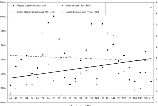
To estimate the effect of the openness and debt levels over the exchange rate adjustment during financial distresses, we present in Figure 1 the currency depreciation3observed versus the degree of openness4and versus the external debt related taxes for the selected crisis sample. We also present the best linear proxies for both relations. Looking to the Figure 1, one can guess that in most open countries the devaluation required tends to be lesser, even without considering many other important variables in such analysis. It also tends to be lesser under lower external debt to tax ratio.
Figure 2 summarizes uncertainty and we describe it further (uncertainty sub-session). Figures 3 to 14 present results of the model simulation which are detailed in the section 3. They are divided in two blocks. In the first one we use Brazil as a benchmark economy to evaluate some qualitative results from the model, like the optimal fiscal policy function; the crisis zone; how the degree of openness can affect this zone and the devaluation-response; how much degree of openness is required to compensate the negative welfare effect of more vulnerability (more risk premium and/or more external debt); what should be the shock required for the default to be better than the devaluation; and how the degree of openness affects this requirement. In the second, we show aggregate results for all countries, verifying that our model can indicate, in a stylized way, the preferences for default-devaluation options and the magnitude of the currency depreciation required to overcome external crisis.
On a more methodological ground, the possibility that default can be welfare enhancing is in accor-dance with the current bankruptcy literature, which says that it is optimal to have some bankruptcy in equilibrium, contrary to conventional wisdom (see Geanakoplos, Dubey and Shubik Dubey and Shubik (2005), for penalties on the utility function, and Araujo, Páscoa and Torres-Martínez Araujo et al. (2002), for infinite horizon economies). Although, the risk of default should be kept under control. Accordingly, the introduction of national currency and trade rises the possibility of a better bankruptcy technology through devaluation of the national currency, rather than repudiation of the external debt.
In the next section we describe the model and an equilibrium. Section 3 presents the numerical exercises and section 4 concludes.
2. THE MODEL WITH NATIONAL CURRENCY AND TRADE
We extended the Cole and Kehoe model (Cole and Kehoe, 1996) by including debt denominated in national currency and trade. There is only one good in the economy produced with capital,k, inelas-tic labor supply and price normalized to one; three parinelas-ticipants — national consumers, international bankers and the government; public external debt denominated in dollars or indexed to this currency, B∗, and public internal debt denominated in national currency, B. The external public debt is only acquired by international bankers, and there is a positive probability of no rollover whenever its level is in the crisis zone. We consider that any suspension in its payment is permanent and total, as in the original model. On the other hand, public debtBis only taken up by national consumers, which are
3We present details of these calculations and plot in the numerical exercise section and in the Table 3. Note that only
devalua-tions bigger than 30% are selected.
always prone to rolling it over, charging the price associated with the positive probability of partial repayment due to currency devaluation.
2.1. Uncertainty
To characterize uncertainty, we suppose that sunspot variables give a representation of real shocks and not just psychological ones. The model contains two sunspots: one representing the local investors’ confidence,ζ, and another portraying external investors’ confidence in the government,ζ∗, which has uniform distribution on [0;1]. Even though these shocks are not explicitly modeled, the fear of a sud-den fall in a commodity price that represents a big share of exports, of changing in the government preferences about public expenditure, or a political turmoil which contributes to the reversal of inter-national capital flows are examples of shocks that the sunspot variablesζ∗andζaim at representing. To generate extra revenues in response to a reversal of capital inflows the government can default on the dollar debt or else, it might devalue the national currency. Therefore, the realizationζ∗indicates the confidence that international investors have that the government will not default on the dollar debt. Likewise, the sunspotζdescribes the national investors’ confidence that the government will not devalue the national currency.
We consider that the sunspotζ realization is conditional onζ∗ realization. The probability that the international bankers’ confidence is below a critical valueπ∗ is given byP(ζ∗≤π∗) = π∗.If ζ∗ ≤π∗,ζis supposed to be distributed with uniform [0;1], but ifζ∗ > π∗,ζis supposed to be one. The probability that the consumers’ confidence is below the critical valueπgiven that international bankers are not willing to renew their loans isπ,i.e.P[ζ≤π|ζ∗≤π∗] =π. Then, in the model with debt in national currency, the probability of a self-fulfilling external debt crisis occurring isπ∗(1−π), which is equal to[P(ζ∗≤π∗)]·[P(ζ > π|ζ∗≤π∗)]. In this case, there is a suspension of foreign credits and the price that the international bankers are willing to pay for the new dollar debt, q∗, is zero. The fear of default is self-fulfilling. With probabilityπ∗πthere is an external crisis,q∗= 0, but the government devalues its currency in order to avoid the default. In this case both national and foreign creditors have very low confidence that the government will honor its debt obligations. Figure 2 sums up the three possible states in the crisis zone.
To avoid unnecessary technicalities, we rule out from the model the possibility that both default and devaluation can be used together. Instead, we consider that during a crisis each one of them can be used with some positive probability, given by sunspot,ζ. These probabilities can be inferred from the spreads of the interest rates on national currency public debt and on dollar currency public debt over the free risk rate. We also assume that the commitment to no-devaluation (no-inflation) is enforceable when there is no external crisis(q∗ >0). The results presented in the numerical solution (Figure 7) show that for low levels of the external debt, devaluation is the best response in the crisis zone and, for high levels, default is preferable.
2.2. Crises responses and trade openness
The decision to default on the dollar debt is characterized by the government’s decision variable,z∗, being equal to zero from default decision on, or being otherwise equal to one. We assume that default causes a permanent fall in national productivity,a, from1toα, withαǫ(0,1). Meanwhile, the decision whether or not to devalue the national currency is described by the government decision variable,z,
withzǫ(0,1]. On one hand, when international creditors do not renew their loans and the government
response against the crisis and conditional onz∗= 1.5Therefore, devaluation of the national-currency also brings a cost in terms of lower productivity and a benefit of extra revenue that helps to avoid an external default. Finally, provided that there has not been either a default or an inflation tax, previously or at present, thenais equal to one and the government decision variables arez∗ = 1andz = 1. Figure 2 shows the three possible government decisions and implied productivity, depending on the realization of the sunspots and considering external debt in the crisis zone. The crisis zone is defined as the interval of the external debt for which the government prefers to default if(q∗= 0),and not to default if(q∗>0). Both equilibria are possible and the selected one is given by the sunspot variables.
• Real devaluation
We do not model exchange rate transactions explicitly. Instead, we directly model the consequences of an exchange rate devaluation. Accordingly, it reduces the international value of a bond denominated in the devalued currency and it improves the trade balance. We also keep our framework based on a single good as in the original model. We assumed that the indebted country produces goods locally, and such goods have its price normalized to unity. When such good is exchanged abroad, its price changes. Therefore, there is only one good but with different prices depending on the place it is traded. This trade could be thought of as occurring through an exchange rate market. The government budget constraint in each period(t), in units of the domestic goods, is given by:
gt≤θ.[atf(Kt)−δKt] +T Bt−Rt−1zt∗Bt∗+Rtq∗tBt∗+1−Btzt+Bt+1qt (1)
withgbeing the public expenditure,θbeing the tax rate,f(.)6 being the production function,Kis the capital stock of the economy,Ris the price of the domestic good when it is exchanged abroad,δ is the depreciation factor,T Btis the trade balance andq,q∗are the prices of the national currency-denominated bond in unit of domestic goods and the dollar-currency-denominated bond in units of domestic goods traded abroad, respectively.
We suppose that every country’s international transaction occurs through the government budget constraint (1). This way, the imbalances in the current account,(−T Bt),plus the imbalances in the nonreserve capital account, Rt−1z∗tBt∗−Rtqt∗Bt∗+1
, are compensated by official reserve transactions, which cause a reduction in the public expenditure(g). We also assume that the nominal exchange rate is fixed or pegged to another currency, but might suffer a significant devaluation after the realization of an external shock. National governments may choose to devalue the national-currency in order to make local goods cheaper, impacting the trade balance,T Bt, and the return of its debts. As long as the pass-through coefficient from nominal exchange rate to prices,τ,is less than one, the devaluation is followed by a rise in the real exchange rate,R, and a rise in the domestic inflation, which implies that zis less than one,i.e.z=φ(τ). In this case, the government paysφBto local investors, reducing the real return on the national-currency debt. Furthermore, the real devaluation increases the volume of exports and decreases the demand for both imports and new dollar debt. We consider that it does not increase the price to be paid for the old external debt as the government can pay it before changingR. Then, the advantages of the devaluation-response embrace avoiding an external default, reducing the national-currency debt to GDP ratio; sinceφB, instead ofB, is settled from the moment of the devaluation on; and improving the trade balance. All these gains should be weighed up in terms of welfare. On the other hand, there are costs related to the inflation tax and to the rise in the value of the foreign obligations.
5We consider that this best-response is also permanent, i.e. ifz
t=φ <1thenzt+i=φ∀i≥0.Then, there is a permanent
and constant inflation rate equal to1−φφafter devaluation. Real effects over local public debt return and real exchange rate is present in the first period after devaluation. From the second period on, inflation is predictable and affects only nominal variables.
To compute such effects in the trade balance, we consider that its value,T B(R),depends on the real exchange rate. At times of no external crisis,Ris equal to one and the trade balance enters as a constant term in the government budget constraint. We are only interested in the revenue that the government obtains from an improvement in the trade balance after a real devaluation,D(R).7 This revenue depends on the intensity of the real devaluation, the trade volumes, and the real-exchange-rate elasticities of exports and imports,ηandη∗, respectively,8as developed in the Appendix. We setD(R) as
D(R) = (R−1) (ση+η∗R−1)Imp(1)
where(R−1)is the rate of devaluation,σis the export-import ratio andImp(1)is the initial level of imports whenR = 1. Then, a devaluation produces a positive change in the trade balance as long as (ση+η∗R)is greater than one, which means that the trade account is improved when the response of export-import ratio to a change of the real exchange rate is preponderant. In this case, the more price-elastic the trade volumes are, the greater the improvement will be. Note that the devaluation also may worsen the trade account because of the negative wealth effect on the import volumes ordered before the change in the real exchange rate.
2.3. Market participants
At any timet, the representative consumer maximizes the expected utility
max {ct,kt+1,bt+1}t
E ∞
X
t=0
βt[c
t+v(gt)]
subject to the budget constraint, given by
ct+kt+1−kt+qtbt+1≤[at.f(kt)−δkt] (1−θ) +bt−bt(1−zt)
givenk0>0andb0>0. At timet,the consumer chooses how many goods to save for the next period,
kt+1, to consume at present,ct, and the amount of new national-currency debt to buy, bt+1, which
consists of zero-coupon bonds maturing in one period. The utility has two parts: a linear function of private consumption, ct, and a logarithmic function of government spending, v(gt) ≡ ln(gt). The right-hand side of the budget constraint corresponds to the sum of consumer’s income from produc-tion, after taxes and capital depreciaproduc-tion, plus the return on the national-currency debt acquired in the previous period. If there is no devaluation,ztequals to one and this return equals tobtdomestic goods.
Analogously, at any timet, the problem of the representative international banker is
max {xt,b∗t+1}t
E ∞
X
t=0
βtxt
subject to the budget constraint
xt+Rtq∗tb
∗
t+1≤x+Rt−1zt∗b ∗ t
givenb∗
0>0. At timet, the bankers choose how many goods to consume,xt, and the amount of new government bonds denominated in dollar to buy,b∗
t+1. The expenditure on new government debt is
Rtq∗tb∗t+1, whereq∗t is the price of the zero-coupon bond that pays one unit of good at the maturity (t+ 1)if the government does not default. The right-hand side includes the revenue received from
7T B(R >1)−T B(1).
the bonds purchased in the previous period,Rt−1zt∗b∗t,and the fixed endowment flow,x. The decision variablez∗indicates whether the government defaults (z∗ = 0) or not (z∗= 1). If it defaults, then the bankers receive nothing.
The government is assumed to be benevolent in the sense that it maximizes the welfare of national consumers, with no commitment to honor its obligations. Its budget constraint is given by (1), where the left-hand-side is the government’s consumption and the right-hand-side includes the following terms: the income tax, the trade balance and the interest paid both on the dollar debt and on the national-currency debt.
In order to obtain the real exchange rate as a function of the government inflation decision, we define the real exchange rate devaluation as:
∆R
R =
∆E
E +
∆P∗
P∗ −
∆P P
Assuming that the foreign price levelP∗is constant, we obtain the local-inflation rateκ:
∆P
P =
τ 1−τ
∆R R
with the pass-through from nominal exchange rate change to local prices,τ,being equal to ∆PP/ ∆E E
. The value ofz,which corresponds to the units of domestic goods that a national-currency bond actual pays at maturity, is defined as
z= 1
1 +κ
Because we consider only the devaluation possibility, i.e.Rt+1≥Rt,we havezǫ(0,1].Accordingly, we arrive at an expression that relateszto the change in the real exchange rate:
z=
1 + (R−1) τ (1−τ)
−1
(2)
where the devaluation rate is given by(R−1),sinceR0= 1.
The government is assumed to behave strategically as it can foresee the optimal decisions of all market participants; including its own,z∗
t,ztandgt; given the initial aggregate state of the economy and its choices ofB∗t+1andBt+1. To match aggregate and individual variables it is assumed that, in
the initial period, the supply of dollar debtB∗
0 is equal to the demand for this debt,b∗0; the supply of
national currency debtB0is equal to its demand,b0; and the aggregate capital stock per worker,K0, is
equal to the individual capital stock,k0. The population of both consumers and bankers is continuous
and normalized to unit.
2.4. A recursive equilibrium
The definition of a recursive equilibrium follows the same procedure developed by Cole and Kehoe (Cole and Kehoe, 1996). The actions of the participants are taken backwards according to the timing in each period.
Timing of actions within a period
• the sunspot variablesζ∗ andζ are realized and the aggregate state of the economy iss≡(K,
B∗,B,a−
1,ζ∗,ζ);
• the government, taking the national-currency bond price schedule,q =q(s,B∗′,B′) as given, chooses the new national-currency debt,B′;
• international bankers, takingq∗andz∗as given, choose whether to purchaseB∗′;
• local investors, consideringq∗,qandzas given, decide whether to acquireB′;
• the government decides whether or not to default on dollar debt,z∗;
• the government decides whether or not to devalue the national currency, z, and chooses its current consumption,g;
• consumers, takinga(s,z∗,z)as given, choosecandk′.
Given this timing of actions, we can work backward in each period to define the value functions and the states variables for each market participant, starting with consumers who move last. For simplicity, from now on, we refer to consumers and government decisions asCandG,respectively.9
Each consumer knows the stock of capital saved,k, the stock of national-currency debt purchased,
b, the aggregate state of the economys, and the new dollar and national-currency debts offered by the
government,B∗′andB′. GivensandB∗′, consumers take as given the price that international bankers are willing to pay for the new dollar debt,q∗(s,B∗′,B′), and the price that turns them indifferent to accepting or not the new national-currency debt,q(s,B∗′,B′).They are also able to anticipate the gov-ernment’s decisions for the coming period,G(s′). Therefore, when consumers choose the amount of new national-currency debt,b′, their state iss
c≡(k,b,s,G(s)). The value function for the representa-tive consumer is given by:
Vc(sc) = max
c,k′,b′{c+v(g) +EVc(s ′
c)} (3)
s.t. : c+k′−k+qb′≤(1−θ) [af(k)−δk] +zb; (c,k′)>0.
Each international banker decides how much public debtb∗′to buy, knowing the amount of dollar debt purchased in the previous period,b∗, the aggregate state,s, and the government’s decisionG(s). They also take prices as given,q(s,B∗′,B′)andq∗(s,B∗′,B′), and the government decisions for the coming periodG(s′).Accordingly, their state issb≡(b∗,s,G(s))and their value function is defined by:
Vb(sb) = max
x,b∗′ x+βEVb(s ′
b) (4)
s.t. : x+Rq∗b∗′≤x+R−1z∗b∗; x≥0
The subscript(−1)indicates that whenq∗ = 0and the government choose to devalue, it can pay
the old debt first.
Finally, the government makes decisions twice within a period. When it chooses its new debt levels, it knows the states. Moreover, it takes price schedulesq∗(s,B∗′,B′) andq(s,B∗′,B′) as given, as well as its optimal choices induced by the new debts,G(s′|B′,B∗′). Likewise, the government also recognizes that it can affect the optimal choices of consumers,C(sc), the price schedulesq∗(s,B∗′,B′)
andq(s,B∗′,B′), and the productivitya(s,z∗,z)of the economy.
Then, in the beginning of each period, the government choosesB∗′andB′, and its value function is defined by
Vg(s) = max
B∗′,B′ c(sc) +v(g) +βEVg(s
′)
(5)
s.t. : g=g(sg) ; z∗=z∗(sg) ; z=z(sg)
where the last three restrictions indicate that the government chooses the best actions given its pre-vious choices about the debt level. sg is defined as the state of the government,(s,B∗′,B′). There-fore, after national and international investors decide about buying new debt, the government decides whether or not to default and whether or not to devalue the national currency. By comparing wel-fare levels according to repayments decisions, and taking all debt levels as given, the policy functions
z∗(s
g),z(sg)andg(sg), are solutions for:
max
z∗(s),z(s),gc(sc) +v(g) +βEVg(s
′)
(6)
subject to,
g+z∗R(−1)B∗+zB ≤ θ[a(s,z∗,z)f(K)−δK] +T B(R) +q
∗
RB∗′+qB′
g ≥ 0,zǫ(0,1] 0 = (R−1) (1−z∗)
where the last restriction indicates that default and devaluation cannot be implemented at the same time. We defined z and z∗ as function of sbecause when to default is better than not to default (z∗= 0≻g z∗= 1|z= 1), then the actual government response to the crisis, namely devaluation or default, depends on the sunspot-ζrealization. We also consider that when devaluation is used to avoid the default,zis chosen to maximize the welfare conditional toz∗= 1.
Definition of an equilibrium
An equilibrium is defined as a list of value functionsVcfor the representative consumer,Vbfor the representative international banker, andVgfor the government; policy functionsCfor the consumer, b∗′, for the international banker, andGfor the government; price functions for the dollar debt,q∗, and for the national-currency debt,q; and an equation for the aggregate capital motion,K′, as follows:
(i) givenG,q,q∗;V
cis the value function for the solution to the problem of the consumers (3), and Care their optimal choices;
(ii) givenG,q,q∗;V
bis the value function for the solution to the problem of the international bankers (4), andb∗′is their optimal choice;
(iii) givenC,q,q∗;V
gis the value function for the solution to the problem of the government (5 and 6) andGare its optimal choices;
(iv) B∗′(s)∈b∗′(s b);
(vi) B′(s)∈b′(s c);
(vii) K′(s,G(s)) =k′(s c).
2.5. Equilibrium Analysis
The behavior of consumers and bankers depends on their expectations regarding whether or not the government will default on the dollar debt or create inflation tax on the national-currency debt through devaluation. On the other hand, the government actions also depend on these expectations which have real effects through the debt prices and investment levels.
next period, and to the possibility that this crisis results in a default or a currency devaluation. Then, the optimal capital accumulation, kt+1, depends on the consumers’ expectations about productivity,
Et[at+1],as follows:
1
β = 1 + (1−θ) [f′(kt+1)E(at+1)−δ]
Furthermore, consumers act competitively and are risk neutral, so they may purchase new public debt denominated in national-currency if its price equals the expected return to1/β:
1
β =
Et[zt+1]
qt
The more closed the economy is the greater is the devaluation (inflation) required during the crisis and the smaller is the expected value forzt+1.So, interpreting q1t as being the interest factor over the
national currency debt we can say that the interest rate is decreasing in the degree of openness. Analogously, international bankers act competitively and are risk neutral, so they may purchase new public debt denominated in dollar-currency if its price equals the expected return to1/β:
1
β =
Et
z∗
t+1
q∗
t
During a crisis(ς∗< π∗) they are convinced about default on the next period and so they set
q∗
t = 0.
Finally, to complete the equilibrium analysis we must find which are the government actions. Let-ting Vg(s|z,z∗,q∗)denote the payoff to the government conditional on its decisions, zand z∗, and conditional on the priceq∗,and also considering that the public debt level denominated in the national currency cannot change over time(Bt=Bo∀t),10it is possible to construct an equilibrium with the crisis zone defined by the external debt level as in the Cole Kehoe model (Cole and Kehoe, 1996).
Next, we define theparticipation conditionwhich ensures that the government will want to honor the current external debt given it is able to sell new one:
Vg(s|1,1,q∗>0)> Vg(s|1,0,q∗>0) (7)
Analogously, we define theno-lending conditionwhich ensures that the government will want to default during a crisis:
Vg(s|1,0,q∗= 0)> Vg(s|1,1,q∗= 0) (8)
The crisis zone is defined as the interval for the current external debt level,(b,B],wherebis the greatest external debt level so as equation (8) does not hold with (b,kn)ǫs,
and B is the greatest external debt level so as equation (7) holds for B,kπ∗π
ǫs. When the economy is out of the crisis zone, i.e.B∗≤b,there is always external credit available. Since the bankers know that the government would not to default even if the price were zero, they do not refuse to rollover new bonds. In the crisis zone the bankers are aware of the possibility of default, and may refuse to sell new bonds(q∗= 0). In this case, default is desirable, but with probabilityπthe government devalues to avoid the default.
Although we do not compare the payoffs of devaluationversusdefault to characterize the crisis zone (we maintain the possibility of both responses occur), we compute in the numerical exercises, presented in the next section, the level of external debt,eb, for which government would be indifferent between
10From now on we consider that this assumption holds. Otherwise, there would be no external crisis since the absence of new
default and devaluation. We also verify thatebǫ(b,B)and that devaluation is the best response in the crisis zone ifB∗<eb.IfB∗>eb,default is the best response in the crisis zone.
Table 1 presents the four possible equilibrium capital accumulation and prices, according to the expectations. In the first line of the table we consider that the external debt is out of the crisis zone. In the second one we consider that the external debt level is in the crisis zone and the two last present the values for the after-crisis economy. Each one of the three last lines corresponds to the three states characterized in Figure 2.
3. NUMERICAL EXERCISES
In this section, we first present numerical exercises for the Brazilian economy to show some qualita-tive results from the model. Secondly, we present aggregate results for 58 currency crises and attempt to outline some of the factors that make countries adopt different crisis responses, with more or less devaluation, and choosing default or not.
3.1. Qualitative results
The parameters used in the simulations have been chosen to portray the Brazilian economy during 1998, period that precedes the Brazilian currency devaluation, starting in January 99. The definition of period length is based on the Brazilian government debt whose average length was varied from 7 to 10 months between 98-99. The government discount factor,β, is approximated by the yearly yield on government bond issued by the US, whose values were about 5 percent. Based on these figures, we interpret a period length as being one year and a yearly yield on risk free bonds,r,as being0.05, which implies a discount factorβ of0.95(= (1 +r)−1). The choice of the functional forms forv(.) and f(.)were the same used by Cole and Kehoe Cole and Kehoe (1996), that is,v(g) = ln(g)and f(k) = Akλwhere capital shareλis established at0.4and the scale factor at10. The parameterα equals0.95,assuming that default causes a permanent drop in productivity of0.05. Forz = φ,the correspondent inflation rate is(1−φ)/φ,which implies the welfare cost of inflation,αφ,
estimated according to Simonsen and Cysne11(Cysne and Simonsen, 1994). The probability of default,π∗(1−π), and the probability of inflation,π∗(π), are calculated on the basis of the risk premium practiced in the financial market according to the following expression:
1
β = 1 +r BR D
(1−π∗(1−π)) = 1 +rBR
LC
(1−(π∗π) (1−φ))
whererBR
D andrBRLC are yearly yields on Brazilian public debt denominated, respectively, in dollar and in national currency (discounting the expected inflation of Brazilian currency), andφis given by the unexpected yearly inflation associated with devaluation.
Data forrBR
D are available for the period of analysis, whilerLCBRonly since January 2002, when its value was about 0.12.12 Therefore, considering the values forφ, rBR
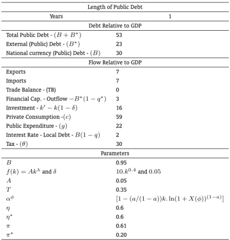
D ,andrBRLC equals to0.5,0.14, and0.12, respectively, we can compute(π∗,π)as being equal to(0.2,0.61). In Table 2 we present the values of parameters and variables used in the simulations for the Brazilian economy, whose results are described next.
Figure 3 shows that when the external public debt is in the crisis zone the optimal policy is to move out from it. But it may be difficult to reduce public expenditure and Figure 4 shows that an alternative
11In the estimation of welfare cost of inflation we use Bailey’s approximation and the money demand specified askr−a, where
ris the logarithmic annual inflation (see Cysne and Simonsen, 1994). We setkandaequals to0.07and0.6,respectively.
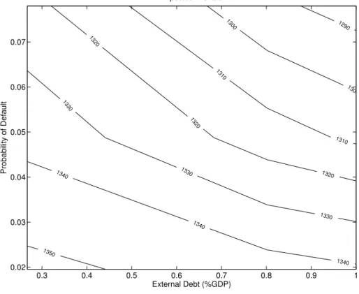
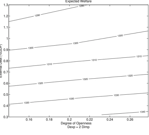
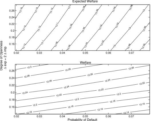
policy could be lengthening the maturity.13These conclusions remain the same as in the original model. Figures 5, 6, and 7 present the effects of the degree of openness over the economy. As shown in Figure 5, if the economy has its imports and exports enlarged without changing the trade balance, i.e. the gains in the volume of exports (Dexp) equal the gains in the volume of imports (Dimp), then only the cap of the crisis zone becomes greater. But if the economy can improve its trade technology and enlarge exports faster than imports, then the international capital inflow becomes greater and both the floor and the cap increases. In figure 6 it is possible to see that, according to the model, the devaluation required to overcome a crisis is increasing in the external debt level and decreasing in the degree of openness. Figure 7 also shows that the “devaluation–better-than-default” region is increasing in the degree of openness. Finally, figures 8, 9, and 10 correspond to welfare analyses. They show how much debt must be paid to compensate the welfare loss related to an increase in the external risk, and how much improvement in the trade is required to compensate the welfare loss related to an increase in both the external risk and the external debt. Note that in Figure 10 both expected welfare and welfare after crisis are considered.
3.2. Cross country results
The parameters used in the simulations for the other countries are presented in Table 3. To compare results across countries we change only a few parameters which we consider more relevant to explain differences between economies and their responses to crisis. The variables that are not presented in Table 3 are the same for all countries including Brazil (Table 2).
Figure 11 shows that, according to the assumptions of our model, the “countries on the left side” were more prone to choosing default than the “ones on the right”. Results match85%of the crises with “reality” in predicting that default is the best response whenever it actually occurs and it is not the best response whenever it does not occur. Triangule marks show where the model failed.
Figure 12 presents the estimated devaluations for different pass-through values. Note that the results are quite similar to a wide range of this parameter. Devaluation rates change significantly only when considering that pass-through is very close to one.
Figure 13 compares actual devaluations and those predicted by the model. In the first plot the elas-ticities(η∗,η)of0.6were considered, and in the second plot we double this value. Note that for greater elasticity less devaluation is required to overcome the external crisis as expected. Accordingly, most de-valuations predicted are overestimated, but not too far from reality. Moreover, we do not consider that our numerical exercise is a good predictor for actual devaluation, since we have made simplifications to compute after-crisis payoffs as considering z∗
t+i= 0,zt+i=φfor alli >0,respectively, in default and devaluation responses. Our aim is to outline the different crisis responses adopted by countries considering factors as the degree of openness, debt levels in both currencies, taxes, and risk-premiums. In this sense, we are more interested in comparing the shape of predicted versus actual devaluations plots.
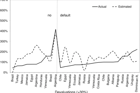
Figure 14 replicates Figure 13 excluding the devaluations lesser than 30% and separating countries that experienced default from the others.
Finally, it is also important to note that there are many ways to compute the actual devaluations of the currencies across countries. We use the exchange rate series published by IMF-Statistics, con-sidering the bilateral price of the dollar related to the national currency, and the mean value for each month. Sudden and significant devaluations indicate the beginning of the crisis period, whose length is defined as six months for all crises. The new level of the exchange rate is considered as the mean of
13We follow Cole and Kehoe approach for “lengthening the maturity structure”. Henceforth, lengthening the maturity
struc-ture means converting an initial quantityB∗of one-period (one year) bonds into equal quantitiesB∗
nof bonds of maturity
n(1,2, . . . ,N). Then, the government redeemsB∗
nbonds every period and sellsBn∗n-period bonds, whereB∗n(1−qn∗) =
B∗(1−q∗),andq∗
the exchange rate for this crisis period and the actual devaluation for each country is computed as from the exchange rate level immediately before the crisis period.
4. REMARKS
As Cole and Kehoe already pointed out, this type of model differs from most of the literature on debt crises by using a dynamic stochastic general equilibrium framework with an altruistic government rather than using a deterministic model or a model with a reduced form for the government. We extended their original debt crisis model by adding trade and local debt, without losing neither the dynamic stochastic general equilibrium framework nor the altruistic government. Original qualitative results remain in our extended version, i.e. the policy recommendation in almost all cases is to leave the crisis zone through both fiscal adjustments and through lengthening the maturity of the external debt. As a novelty, we present the positive welfare effect from trade openness and how it shifts the crisis zone up. Finally, we predicted, in a stylized way, the relative magnitude of the national currency depreciation required to overcome external crises and the preferences for default-devaluation options.
BIBLIOGRAPHY
Araujo, A. & Leon, M. (2002). Ataques especulativos sobre dívidas e dolarização. Revista Brasileira de Economia, 56(1):7–46.
Araujo, A., Leon, M., & Santos, R. (2006). Monetary arrangements for emerging economies.
Araujo, A., Páscoa, M., & Torres-Martínez, J. P. (2002). Collateral avoids Ponzi schemes in incomplete markets.Econometrica, 70(4):1613–1638.
Calvo, G. (2000). The case for Hard Pegs. Mimeographed, University of Maryland.
Calvo, G., Izquierdo, A., & Talvi, E. (2003). Sudden stops, the real exchange rate, and fiscal sustainability: Argentina’s lessons. Working Paper No. 9828 July 2003.
Chang, R. & Velasco, A. (2000). Exchange rate policies for developing countries. American Association Papers and Proceedings, 90:71–75.
Cole, H. & Kehoe, T. (1996). A self-fulfilling model of Mexico’s 1994-1995 debt crises. Journal of Interna-tional Economics, 41:309–330.
Cole, H. & Kehoe, T. (1998). Self-fulfilling debt crises. Staff Report.
Cole, H. & Kehoe, T. (2000). Self-fulfilling debt crises.
Cysne, R. & Simonsen, M. (1994). Welfare costs of inflation: The case for interest-bearing money and empirical estimates for Brazil. Ensaios Econômicos, 245.
Dornbush, R. (2000). Millenium resolution: No more funny money. January.
Dubey, P.; Geanakoplos, J. & Shubik, M. (2005). Default and punishment in general equilibrium. Econo-metrica, 73(1).
Frankel, J. (1999). No single currency regime is right for all countries or at all times. Cambridge, Mass 7338, National Bureau of Exonomic Research. W.P.
Mishkin, F. (1998). The dangers of exchange rate pegging in emerging market countries. International Finance, 1(81):101.
Mussa, M., Masson, P., A., S., Jadresic, E., & Mauro, P.; Berg, A. (2000). Exchange rate regimes in an increasingly integrated world economy. Washington,D.C.
Paiva, C. (2003). Trade elasticities and market expectations in Brazil. WP/03/140, Jul. 2003.
Reinhart, C. K., Rogoff, K., & Savastano, M. (2003). Debt intolerance. August 2003.
Sachs, J. & Larrain, F. (1999). Why dollarization is more straitjacket than salvation. Foreign Policy, 116:80–92.
5. FIGURES AND TABLES
Figure 1
0 1 2 3 4 5 6 7 8 9
-10% 10% 30% 50% 70% 90% 110% 130%
44 47 57 64 64 65 74 74 78 79 79 80 83 91 98 100 100 100 101 104 157 157 158 158 200 223 417
Devaluation (>30%)
Figure 2
1-
*
*
1-
z* = 1
z = Φ
a = αΦ
z* = 0
z = 1
a = α
z* = 1
z = 1
Figure 3
0 0.1 0.2 0.3 0.4 0.5 0.6 0.7
0 0.1 0.2 0.3 0.4 0.5 0.6 0.7
External Debt Level (%GDP)
Figure 4
5
10
15
20
25
30
35
40
0.2
0.4
0.6
0.8
1
1.2
1.4
1.6
1.8
Average Maturity of the External Debt Level (years)
Level of the External Debt (%GDP)
Crises Zone
Figure 5
1 2 3 4 5
0.2 0.3 0.4 0.5 0.6 0.7 0.8 0.9 1
Average Maturity of the External Debt Level (years)
1 2 3 4 5
0.2 0.3 0.4 0.5 0.6 0.7 0.8 0.9 1
Level of the External Debt (%GDP)
Crises Zone
2x more open imp = exp
Figure 6
0
0.1
0.2
0.3
0.4
0.5
0
0.5
1
1.5
2
2.5
Optimal Devaluation under Attack: calibrated as of Brazilian economy
External Debt (%GDP)
Rate of Devaluation
2x more open imp = exp
Figure 7
0.2 0.25 0.3 0.35 0.4
Openness, exp = 2 imp
External Debt Level (% GDP)
Debt Level for Default-Devaluation Indifference
0.16 0.18 0.2 0.22 0.24 0.26 0.28
0.2 0.22 0.24 0.26 0.28 0.3 0.32 0.34
Openness, exp= imp
Default
Out of Crisis Zone
Out of Crisis Zone Devaluation
Default Devaluation
Devaluation
Default
Default
Figure 8
1290 1300
1300 1310
1310 13
20
1320
1320 1330
1330
1330
1340 1340
1340
1350
Probability of Default
External Debt (%GDP) Expected Welfare
0.3 0.4 0.5 0.6 0.7 0.8 0.9 1
Figure 9
1290
1290
1300
1300
1300
1310
1310
1310
1320
1320
1320
1330
1330
1330
1340
External Debt (%GDP)
Degree of Openness Dexp = 2 Dimp Expected Welfare
0.16 0.18 0.2 0.22 0.24 0.26
Figure 10 12 .96 12 .98 12. 98 13 13 13 13 .02 13 .02 13 .02 13 .04 13 .04 13 .04 13 .06 13 .06 13 .06 13 .08 13 .08 13 .08 13 .1 13 .1 13 .1 13 .12 13 .12 13. 12 13 .14 13 .14 13 .16 Expected Welfare
0.02 0.03 0.04 0.05 0.06 0.07
0.16 0.18 0.2 0.22 0.24 0.26 12.14 12.16 12.16 12.18 12.18 12.18 12.2 12.2 12.2 12.22 12.22 12.22 12.24 12.24 12.24 12.26 12.26 12.26 12.28 12.28 12.3
Probability of Default
Degree of Openness
exp = 2
imp
Welfare
0.02 0.03 0.04 0.05 0.06 0.07
Aloisio Araujo , Mar cia Leon and Rafael Santos Figur e 11
0 2 4 6 8 10
Guyana Egypt Morocco Morocco Bolivia Philippines Costa Rica Ecuador Albania Chile Argentina Mexico Ecuador Russia Chile Venezuela Paraguay Uruguay Chile Jamaica Jordan Bulgaria Trinidad T. Venezuela Jamaica Honduras Brazil Egypt Argentina Russia Romania Philippines Swaziland Papua N. G. Costa Rica Mexico Venezuela Thailand Malasya Turkey Argentina Gabon Botswana Dominican R. Mexico Singapore Brazil default > devaluation default < devaluation (Actual External
Public Debt)-to-(External Public
Debt for Default-Devaluation Indifference)
Figure 13
-100% 0% 100% 200% 300% 400% 500%
Albania
Arg
entina Boli
via
Bra
z
il
Bulgaria
Chile
Costa Ri
ca
Dom
inican R. Ecuador
Egypt
Guyana Jamaic
a
Jor
d
an
Malasy
a
Mexic
o
Morocc
o
Papua
N. G.
Philippines Rom
ania
Russi
a
Swazilan
d
Tr
in
ida
d
T.
Ur
uguay
Venezuela
Full Sample
Actual Devaluation
Estimated , First Plot (elast=0.6)
Figure 14
0% 100% 200% 300% 400% 500% 600% 700%
Devaluations (>30%)
Actual Estimated
Table 1: Equilibrium Prices and Investment
K′(E(a
t+1)) q(Ez) q∗(Ez∗)
K′(1) β β
Kπ∗π(π∗παφ+π∗(1−π)α+ (1−π∗)) β.{1−π∗π(1−φ)} β{1−π∗(1−π)}
Kφ(αφ) β.φ β
Kd(α) β 0
Table 2: Brazil(98)-Before Exchange Rate Devaluation
Length of Public Debt
Years 1
Debt Relative to GDP
Total Public Debt -(B+B∗) 53
External (Public) Debt -(B∗) 23
National currency (Public) Debt -(B) 30
Flow Relative to GDP
Exports 7
Imports 7
Trade Balance - (TB) 0
Financial Cap. - Outflow−B∗(1−q∗) 3
Investment -k′−k(1−δ) 16
Private Consumption -(c) 59
Public Expenditure -(g) 22
Interest Rate - Local Debt -B(1−q) 2
Tax -(θ) 30
Parameters
B 0.95
f(k) =Akλandδ 10.k0.4and0.05
A 0.05
T 0.35
αφ [1−(a/(1−a))k.ln(1 +X(φ))(1−a)]
η 0.6
η∗ 0.6
π 0.61
π∗ 0.20
Speculative
A
ttacks,
Openness
and
Crises
ind
(y/m) Episode
Albania 1992 7 y 1992 100 11 89 21 67 0 5 15 30 25 y
Argentina 2001 12 y 2001 158 12 10 12 39 16 5 5 78 15 n
Argentina 1989 11 n 417 13 7 10 83 40 3 66 95 90 y
Argentina 1990 12 n 80 10 5 10 43 17 6 6 87 92 y
Bolivia 1989 7 y 1988 9 22 23 13 83 4 5 40 67 16 n
Botswana 1975 7 n 1976 20 44 64 30 39 19 3 3 49 94 y
Brazil 1998 12 n 44 7 7 30 23 30 5 20 61 24 n
Brazil 1993 6 n 1992 158 11 9 26 29 62 5 9 94 96 y
Bulgaria 1992 12 y 1992 100 47 53 36 114 115 12 55 65 90 y
Chile 1984 8 y 1985 30 24 25 29 69 25 5 31 75 26 n
Chile 1971 12 y 1972 100 11 12 15 25 21 8 37 67 12 n
Chile 1982 5 y 1983 47 19 21 29 35 4 8 30 60 26 n
Costa Rica 1987 8 y 1987 8 32 36 21 98 18 5 19 90 25 n
Costa Rica 1980 12 y 1981 98 26 37 17 48 28 8 7 33 82 y
Dominican R. 1984 12 y 1982 223 28 33 11 29 19 9 85 60 80 y
Ecuador 1999 9 y 1999 74 32 25 14 88 9 7 15 76 30 n
Ecuador 1982 4 y 1982 29 22 24 11 44 0 3 37 65 18 n
Egypt 1989 7 y 1987 57 18 32 29 112 74 7 8 93 8 n
Egypt 1978 12 n 79 22 37 38 86 62 8 13 60 90 y
Gabon 1980 9 y 1978 12 65 32 36 35 4 14 23 50 77 n
Guyana 1983 12 y 1982 24 46 65 43 255 193 6 16 60 10 n
Honduras 1990 2 n 101 29 34 15 93 16 8 4 84 89 y
Jamaica 1991 8 y 1990 74 50 51 32 111 0 7 6 88 82 n
Jamaica 1983 10 n 79 36 43 25 94 54 6 13 67 90 y
Jordan 1988 8 y 1989 27 45 67 14 98 52 3 16 25 73 y
Korea 1997 6 n 15 35 36 17 11 1 8 10 67 41 n
Malasya 1985 12 n 5 54 49 27 54 30 8 4 73 112 y
Mexico 1982 2 y 1982 83 10 13 14 27 29 9 3 87 11 n
Mexico 1989 1 n 5 20 19 13 51 27 5 6 74 92 y
Continued on Next Page
RBE
Rio
de
Janeiro
v.
66
n.
2
/
p.
135–165
Abr
-Jun
Aloisio
Araujo
,
Mar
cia
Leon
and
Rafael
Santos
Table 3
Country
Currency Crises Debt Default1
Actual devaluation EXP/GDP(%) IMP/GDP(%) TAX/GDP(%) B∗/GDP(%) B/GDP(%) Free risk(%) π∗(%) π(%) b
ind/GDP(%)2 3
Start of Episode of
(y/m) Episode
Mexico 1994 11 n 65 17 22 13 29 8 4 18 70 86 y
Morocco 1984 11 y 1985 7 24 34 24 108 32 7 7 52 16 n
Morocco 1983 7 y 1983 13 21 30 25 92 35 5 15 61 16 n
Papua N. G. 1994 8 n 22 56 38 23 36 16 9 5 35 56 n
Paraguay 1989 2 y 1987 104 34 37 10 59 2 5 22 66 38 n
Philippines 1986 1 y 1986 8 24 22 12 78 16 3 25 54 20 n
Philippines 1983 9 y 1983 27 22 28 12 63 18 8 4 85 83 y
Romania 1996 1 n 13 28 33 30 20 24 8 3 83 26 n
Russia 1998 7 y 1998 157 31 25 20 57 29 5 60 62 26 n
Russia 1992 12 y 1991 78 62 48 16 31 14 8 72 75 35 n
Singapore 1997 7 n 10 131 139 40 17 59 8 3 66 52 n
Swaziland 1985 7 n 28 57 85 29 64 1 6 21 59 88 y
Thailand 1997 3 n 14 48 47 18 41 0 8 4 27 81 n
Trinidad T. 1988 7 y 1989 17 39 34 29 47 17 5 19 78 40 n
Turkey 2001 1 n 64 24 32 28 45 27 5 4 75 96 y
Uruguay 1982 11 y 1983 200 14 17 21 27 18 7 5 79 19 n
Venezuela 1995 11 y 1995 91 27 22 16 43 24 8 25 79 23 n
Venezuela 1984 1 y 1982 64 20 11 22 36 0 3 19 58 33 n
Venezuela 1989 2 n 157 20 27 19 51 5 4 3 67 92 y
To reach comparative results, we set scale factor (A) equals to 15 for all countries, including Brazil. 1: Default or restructuring of the external debt. Many episodes lasted several years. 2: bind is the debt for default-devaluation indifference, and its value split the crisis zone into two. 3: Only to compute the critical debt levels avoiding empty crises zones, in some countries, we consider that government has constant endowment of 0.75 GDP/year. (n) means no endowmentand (y) means 0.75-endowment. Sources: The World Debt Tables, World Bank Book ; International Financial Statistics, Yearbook / IMF ; World Development Indicators, The World Bank ; Country Info Base free available in http://www.dbresearch.de ; Central Banks.
RBE
Rio
de
Janeiro
v.
66
n.
2
/
p.
135–165
Abr
-Jun
A. APPENDIX
A.1. Effect of Real Devaluation on the Trade Balance
DefiningExpas exports measured in domestic output units,Impas imports denominated in units of good traded abroad,R1as the initial real exchange rate, andR2as its new level after devaluation,
we can compute the trade balance changeD(.)as:
T B(R) = Exp(R)−Imp(R)R
∆T B
∆R =
∆Exp
∆R −
∆Imp
∆R R2−Imp(R1) ∆T B
∆R =
∆Exp ∆R
R1
Exp(R1)
Exp(R1)
R1
−∆Imp ∆R
R1
Imp(R1)
R2
Imp(R1)
R1
−Imp(R1)
∆T B
∆R =
η
Exp(R1)
R1·Imp(R1)
+η∗R2
R1
−1
Imp(R1)
Whereη= ∆∆ExpR R1
Exp(R1)andη
∗=−∆Imp
∆R R1
Imp(R1).Definingσas the exports-imports ratio,R1≡1,
andR2≡R, we obtain