ADDRESSING CONGESTION ON SINGLE ALLOCATION HUB-AND-SPOKE NETWORKS
Ricardo Saraiva de Camargo
∗and Gilberto de Miranda Jr.
Received March 28, 2012 / Accepted August 8, 2012
ABSTRACT.When considering hub-and-spoke networks with single allocation, the absence of alternative routes makes this kind of systems specially vulnerable to congestion effects. In order to improve the design of such networks, congestion costs must be addressed. This article deploys two different techniques for ad-dressing congestion on single allocation hub-and-spoke networks: the Generalized Benders Decomposition and the Outer Approximation method. Both methods are able to solve large scale instances. Computational experiments show how the adoption of advanced solution strategies, such as Pareto-optimal cut generation on the Master Problem branch-and-bound tree, may be decisive. They also demonstrate that the solution effort is not only associated with the size of the instances, but also with their combination of the installation and congestion costs.
Keywords: single allocation hub location problem, Benders decomposition method, outer-approximation algorithm, large scale optimization.
1 INTRODUCTION
Hub-and-spoke networks became an important field of discrete location research. The relevance is largely explained by their widespread use in cargo and passengers transportation and telecom-munication systems [5, 16].
In hub-and-spoke networks, direct transportation of flows between pairs of origin-destination nodes is usually extremely costly. As an alternative, flows from different origins but addressed to the same destination can be consolidated at transshipment nodes, known as hubs, prior to be routed, sometimes via other hubs, towards their destinations. Hubs are then responsible for flow aggregation and redistribution. The bundle of flows at the hubs increases the traffic on inter-hub connections, enabling the use of more efficient and higher volume carriers, resulting then in lower per unit transportation costs [47]. Thus economies of scale can be achieved by bulk transportation. Furthermore, hub-and-spoke networks allow lower infrastructure costs and greater overall efficiency of logistics [37].
*Corresponding author
Generally, in the design of hub-and-spoke networks, there is a connection between every hub pair; no two non-hub nodes can be serviced by a direct link; an origin-destination demand is routed through one or at most two hubs; and the economies of scale at inter-hub connections are represented by a discount factor (0 ≤ α ≤1). Usually the main decisions involve the location of hub facilities, the allocation of origin and destination nodes to hubs (formation of the spokes), the establishment of discounted transportation connections and the routing of flows through the network.
Moreover, according to the characteristics considered, different assumptions may be addressed, including: Single or multiple allocation of the non-hub nodes to the installed hubs, the number of hubs to be located may or may not be known beforehand, direct service between non-hub nodes may be enabled, capacity constraints on the amount of traffic a installed hub can handle, consideration of congestion effects at the installed hubs, flow dependent economies of scale on inter-hub connections, and furthermore there may be not a direct connection between every hub pair, implying then an incomplete hub network structure [6] or a network topology where the hubs are connected by means of a spanning tree [18]. A general review of different problems of hub-and-spoke networks can be found at Campbell [14, 15], while a exhaustive survey is present on Campbellet al.[16] and Alumur & Kara [5].
One of these problem variants is the single allocation hub location problem (SAHLP) where each non-hub is allocated to a single hub only, a fixed cost is incurred each time a node is selected to be a hub, and the path connecting each pair of origin-destination nodes has one or two hubs present. When there are no installation costs but the number pof hubs to be located is known beforehand, the problem is named as the single allocation p-hub location problem (SApHLP). As both problems are closely related, they share the same mathematical programming formulations, differentiating only by the presence or not of a constraint establishing thatphubs must be located and a term on the objective function summing the fixed cost of the installed hubs.
Furthermore, while the multiple allocation hub location problem is closely related to the facility location problem [40], the SAHLP is more akin to the quadratic assignment problem [46]. Hence it is harder to handle, requiring different approaches regarding solution techniques and proper formulations.
Among the available mixed integer linear programming formulations [3, 14, 24, 28, 46, 55], two are worthy of notice: the models of Skorin-Kapovet al.[55] and Ernst & Krishnamoorthy [28]. While the first has the tightest linear programming relaxation (optimality gaps smaller than 1%), yielding integer solution values for the integer variables most of the time at the expense of com-puter memory and time; the latter presents a good trade-off between formulation size (fewer variables and constraints) and computer effort to solve it.
Independently of which hub-and-spoke problem is addressed, one of the main overall advantages of such systems is the exploitation of scale economies. However this may induce the formation of networks that tend to overload a small number of hubs, resulting in some inter-hub connections more heavily-utilized than others. This is specially true when single allocations are involved, since the flow leaving from and arriving at a non-hub node goes through only one hub. Hence it is unavoidable to take congestion effects into consideration.
A common way of addressing congestion in SAHLP and SApHLP networks is to limit the amount of traffic a installed hub can handle [7, 8, 20, 30, 41, 44, 52]. Unfortunately, capacity con-straints do not mimic the explosive nature of congestion: the more flow a hub attracts, the harder the handling process becomes, the greater the costs. Usually these costs increase extremely rapid due to queuing and delay effects. Hence, elaborate cost functions are needed such as the one employed by Elhedhli & Hu [26].
Elhedhli & Hu [26] are the first authors to consider explicitly the congestion effects on the ob-jective function for the SApHLP. Using a power-law function widely utilized to estimate delay costs in airport applications [34]. They propose a non-linear formulation where these convex cost functions, that increase rapidly as more traffic flows through the installed hubs, are present on the objective function. They linearize their model utilizing a set of infinite piece-wise linear and tangent hyperplanes, and then solve it by means of a Lagrangian relaxation algorithm. They solve only toy instances (up to 25 nodes) with an average optimality gap close to 1%. The ob-tained solutions have a more balanced overall distribution of flows through the network than the ones attained by disregarding the congestion effects [26].
In this study, instead of linearizing the implied nonlinear formulation, two very efficient algo-rithms based on the Generalized Benders Decomposition (GBD) method [33] and on the Outer Approximation technique (OA) [23, 31, 57] are employed to handle the nonlinear SAHLP under congestion. These algorithms are different from the former deployed for the multiple allocation variant proposed at Camargoet al.[11]. The main contributions of the present article are the proper derivation of pareto-optimal Benders cuts as devised by Papadakos [49], the exploitation of the special structure of the formulation in order to enable the blending of GBD and OA cuts at the same master program, and the implementation of this strategy in a branch-and-cut framework.
Due to the combination of the best features of each method, the proposed scheme is able to solve large instances to optimality. As far as the authors know, there is no previous report of such large problems solved by the OA technique. Furthermore, a fair comparison of both techniques is presented demonstrating the advantages of one method over the other as a function of some of the instance parameters.
2 NOTATION AND FORMULATION
In this section, the SAHLP under congestion is formulated as a mixed integer nonlinear pro-gram (MINLP) using the model of Skorin-Kapovet al.[55] as a starting basis. The formulation requires the following definitions: Let N be the set of demand node locations which exchange flows and letK be the set of candidate nodes to become hubs. UsuallyK ⊆N, but it is assumed henceforth that all demand nodes are candidates to have a installed hub, implyingK ≡N. For all node pairsiand j(i,j ∈N :i6= j),wi j represents the flow demand from origin nodeito des-tination node j which is routed through either one or two installed hubs. Normallywi j 6=wji. Let alsoOi = P
j∈Nwi j and Di = Pj∈Nwji be the total of demand that is originated from and destined to nodei ∈N, respectively.
Further, let fk be the fixed installation cost of a hub at nodek ∈ N and letci j km be the trans-portation cost per unit of flow from nodei to node j routed via hubs at nodeskandm, that is, the standard transportation cost of routei−k−m−j(i,j,k,m∈N). This transportation cost is the composition of three cost segments: ci j km = ci k +αckm+cm j, whereci k andcm j are the standard transportation cost per unit of flow from nodei to hubkand from hubmto node j, andαckmis the discounted standard transportation cost between hubskandm. The discount factor 0≤α≤1 represents the scale economies on the inter-hub connections. If only one hub is present in any given route thenk=mand no discount factor is applied for the routei−k−k−j.
The MINLP uses flow variablesxi j km ≥ 0 to represent the fraction of demandwi j (i,j ∈ N) that is routed through hubskandm(k,m∈ N), in this order; the variablesgkto account for the total flow passing through hubk ∈ N; and the integer variables zi k ∈ {0,1}to indicate if node i ∈Nis allocated to hubk∈N(zi k =1) or not (zi k =0). When a hub is located at nodek∈ N, thenzkk =1; otherwisezkk =0.
The congestion cost function is usually defined as a power-law τk(gk) = a gkbthat increases rapidly as more traffic goes through hub k ∈ K, where the parameters a > 0 and b ≥ 1 are scalars related to the hub features. The function τk(gk)is increasing on[0,+∞), proper convex and smooth, and it is normally used to estimate delay costs in airport applications [34], being already used by Elhedhli & Hu [26] for the same problem. In this research, the adopted power law function is designed to consider congestion effects after a given flow threshold Ŵk (usually set to 70% of the hub nominal capacity) is trespassed. Such function can be written asτk(gk)=a(max{0,gk−Ŵk})bwithout loss of generality, sinceŴkcan be set for any value where the congestion effects start to degrade the network economies of scale.
In the SAHLP, as each non-hub node is allocated to a single installed hub only, demandswi j and
wji are sent over the same route, enabling then the reduction of the number of variablesxi j km in half [54]. Furthermore, as the outgoing and the incoming flows of a non-hub must go and arrive through the same hub, the cost component of local traffic can be written asP
k6=i(Oi+Di)ci kzi k.
Thus enabling the redefinition of the costsci j kmas
These three simple manipulations improve the overall performance of the algorithms here pro-posed. In the remainder of this paper, for the sake of simplicity in presentation, one must consider i,j,k,m∈ Nandi< j. Hence the implied formulation is given as:
minX k
[fkzkk+τk(gk)]+
X
k6=i
(Oi +Di)ci k zi k+X
i<j
X
k6=m
ci j km xi j km (1)
s. t.: X k
zi k=1 ∀i (2)
X
m
xi j km =zi k ∀i < j,k (3)
X
k
xi j km =zj m ∀i < j,m (4)
X
i
(Oi+Di)zi k−X
i<j
(wi j+wji)xi j kk =gk ∀k (5)
zi k ≤zkk ∀i 6=k (6)
xi j km ≥0 ∀i < j,k,m (7)
gk≥0 ∀k (8)
zi k ∈ {0,1} ∀i,k (9)
The objective function (1) minimizes the total cost associated with the demand transportation, the congestion effects and the hub installation costs. Constraints (2) assure that all nodes are allocated to a hub. Constraints (3) guarantee that routes beginning at origin nodei, then passing firstly at hubk, and finishing at destination node j will only exist if nodei is allocated to hub k. Likewise, constraints (4) guarantee that routes beginning at origin i and passing at hubm just before finishing at destination j will only exist if node j is allocated to hubm. Constraints (5) are responsible for accounting the total hub traffic, avoiding the double computation of the local traffic component. Constraints (6) allow a nodei to be allocated to hubkonly if hubkis installed, while (7), (8) and (9) are the non-negativity and the integrality constraints of variables xi j km,gkandzi k, respectively.
Although there are other formulations for the SAHLP [14, 24, 28], the formulation of Skorin-Kapovet al.[55] is chosen because it provides the tightest linear programming bound. This is a key feature, since nonlinear terms tend to weaken any mixed-integer programming formulation, enlarging the integrality gap as the nonlinearities become dominant. The chosen formulation has also a very interesting property: for a fixed feasible vectorz, the formulation is decomposable for eachi−j pair, recalling that the variablesgkcan be recovered by replacingxi j kkbyzi kzj k.
These constraints assume that the hubs may only be overloaded by the incoming flows originated at the non-hub nodes directly allocated to them.
X
i
Oizi k =gk ∀k. (10)
For those applications where the aforementioned assumption does not hold, Ernst & Krish-namoorthy [30] further suggest that the total hub flow gk can be determined by adding the demands destined to the non-hub nodes directly allocated to a given hub, yielding then con-straints (11).
X
i
(Oi+Di)zi k =gk ∀k. (11)
As observed by Labb´eet al.[41], constraints (11) compute the total hub flowgkin a wrong way. For those non-hub nodes which are allocated to the same hub, the flows originated from and destined to them are accounted twice: One time on the parcel Oi and another time on the parcel Di. Labb´eet al.[41] correct this misconception by proposing constraints (5).
Constraints (5) and (10) induce very different optimal networks, as well as require distinct com-putational efforts. In order to illustrate these differences, a small experiment was carried out by optimally solving, via CPLEX 12, the instance AP20.2, with 20 nodes andα=0.2, of the well-known Australian Post (AP) standard data set [28, 30]. The adopted power-law congestion cost function had parametersa =0.01 andb =2. Figure 2 shows how the network design and the required solution time were affected after constraints (10) were exchanged for (5). The attained values for when no congestion is accounted are also shown. Once again constraints (11) are meaningless since they wrongly compute the total hub flow, therefore they were not considered in this experiment.
In Figure 1(a), the total load (gk) of each installed hubs is represented by a bar above the hub’s index. When congestion effects are disregarded, only two hubs (1 and 10) are installed at the optimal solution. When congestion effects are accounted by computing the total hub flow through constraints (10) or (5), the optimal networks have three (hubs 3, 10 and 11) and six (hubs 1, 3, 8, 9, 10 and 11) hubs, respectively. In other words, they have very distinctive optimal infra-structures.
When the computational efforts are observed, the differences are more pronounced. Figure 1(b) presents, in logarithmic scale, the required solution time for the three considered situations. As can be seen, when constraints (5) are utilized, the required solution time is 204 times greater than when using constraints (10). Constraints (5) greatly hardens the problem, because the termxi j kk is a linearization of the product ofzi kzj k, which greatly affects the attained lower bounds during the branch-and-bound search.
(a) Optimal network infra-structure for different forms of accounting the total hub flow.
(b) Computational effort for different forms of accounting the total hub flow.
Figure 1– Comparison for different forms of accounting the total hub flow for instance AP20.2.
The proposed technique blends OA and classical Benders cuts in a straightforwardly manner, since there is no coupling of thegandxvariables on constraints (10). Their algorithm is capable of solving instances up to 200 nodes in reasonable time. Remark that previous articles on the literature solved only small problems up to 25 nodes [26, 27].
Unfortunately, for those practical situations where one needs to account the total hub flow using constraints (5), which are more general, the technique already proposed by Camargoet al.[13] can not be directly applied, due to coupling of theg andxvariables. Furthermore, as far as the authors know, there are no other studies in the literature that address congestion effects deploying constraints (5).
In the light of the aforementioned reasons, this article proposes a new hybrid OA/Benders al-gorithm that exploits the structure of the formulation, and optimally solves instances up to 100 nodes. Further, the method clearly outperforms an implemented GBD [33] algorithm, a well known technique for solving MINLPs.
Moreover, whenever two formulations – one tight and large, and another weak and small–are available for a given problem, the proposed scheme can be applied, if the global utilization of the common resources is accounted using the smaller model and is computed independently of the large scale system variables. This kind of manipulation simplifies the handling of the non-linearities, by confining them to a kind ofsandbox, while uses the large scale system to improve the formulation bounds.
For sake of presentation and understanding of the required concepts of the hybrid technique, the next section is dedicated to the application of the GBD method for the proposed model.
3 GENERALIZED BENDERS DECOMPOSITION
problem manipulation, followed by solution strategies of dualization, outer linearization and relaxation. The complicating variables (integer variables) of the original problem are projected out, resulting into an equivalent model with fewer variables, but many more constraints. When attaining optimality, a large number of these constraints will not be binding, suggesting then a strategy of relaxation that ignores all but a few of these constraints.
Benders proposes a procedure to add these constraints on demand by using two levels of coor-dination. At a higher level, known as master problem (MP), a relaxed version of the original problem having the set of the integer variables and its associated constraints is responsible for fixing the values of these integer variables and for providing a lower bound (LB) for the problem. At a lower level, known as subproblem (SP), the dual of the original problem with the values of the integer variables temporarily fixed by the MP is responsible for rendering a new cut or a Benders cut to be added to the MP and for generating a upper bound (UB) for the problem. The algorithm iterates, solving the MP and the SP one at a time, until the UB and the LB converge towards an optimal solution, if one exists.
Since the pioneering work of Geoffrion & Graves [32], the Benders decomposition method has been successfully deployed in solving large-scale problems: e.g., the uncapacitated network de-sign problem with undirected arcs [43], the locomotive and car asde-signment problem [19] and, more recently, the multiple allocation hub location problem [10–12].
In Sections 3.1, 3.2 and 3.3, formal descriptions of the MP, the associated SP, implementation issues and solution strategies are presented.
3.1 Benders master program
Projecting the problem (1)–(9) onto the space of the z variables results into the equivalent problem:
min z∈Z
X
k
fkzkk+X
k6=i
(Oi+Di)ci k zi k+φ(z)
where Z = {z∈ {0,1} |constraints(2) and (6) hold}andφ (z)is the following SP:
φ(z)= min
(x,g)∈G
X
k
τk(gk)+
X
i<j
X
k6=m
ci j km xi j km
being
G=
(x,g)≥0|constraints (3)–(5) hold .
Since the constraints definingzare enough to ensure feasibility, the SP is bounded. Further, as
techniques. So associating vectors of dual variablesu,v andβ to constraints (3), (4) and (5), respectively, and because there is no duality gap,φ (z)can be re-written as:
φ (z)=max
u,v,β
min
(x,g)∈G
X
k
τk(gk)+
X
i<j
X
k6=m
ci j kmxi j km+X
i<j
X
k,m
ui j kxi j km
X
i<j
X
k,m
vi j mxi j km−
X
i<j
X
k
βk(wi j+wji)xi j kk−
X
k
βkgk
−X
i<j
X
k
ui j kzi k−
X
i<j
X
m
vi j mzj m+
X
i,k
βk(Oi+Di)zi k
Since the supremum is the least upper bound and with the help of variable η ≥ 0, the whole problem (1)–(9) is then equivalent to following MP:
min z∈Z
X
k
fkzkk+X
k6=i
(Oi +Di)ci kzi k+η (12)
s. t.: η≥ min
(x,g)∈G
X
k
τk(gk)+
X
i<j
X
k6=m
ci j km xi j km+X
i<j
X
k,m
ui j kxi j km
X
i<j
X
k,m
vi j mxi j km−
X
i<j
X
k
βk(wi j+wji)xi j kk−
X
k
βkgk
−X
i<j
X
k
ui j kzi k−X
i<j
X
m
vi j mzj m+
X
i,k
βk(Oi +Di)zi k ∀u, v, β (13)
η≥0 (14)
Because a large number of the constraints of the MP (12)–(14) will not be binding when opti-mality is attained, the GBD algorithm solves the MP through a strategy of relaxation that ignores all but a few of the constraints (13). These constraints are then added, via a iterated procedure, to the MP as needed. Thus for a given iterationt, wherez = zt and after the solution of the associated SP and the recovery of the optimal values ofut,vt andβt, the optimal value ofφ(zt)
is given by:
φ (zt)= min
(x,g)∈G
X
k
τk(gk)+
X
i<j
X
k6=m
ci j km xi j km+X
i<j
X
k,m
uti j kxi j km
X
i<j
X
k,m
vi j mt xi j km−X
i<j
X
k
βkt(wi j+wji)xi j kk−
X
k
βktgk
−X
i<j
X
k
uti j kzti k−X
i<j
X
m
vi j mt ztj m+X
i,k
Further, constraints (13) can be rewritten for iterationtin the form:
η≥ min
(x,g)∈G
X
k
τk(gk)+
X
i<j
X
k6=m
ci j km xi j km+X
i<j
X
k,m
uti j kxi j km
X
i<j
X
k,m
vti j mxi j km−X
i<j
X
k
βkt(wi j+wji)xi j kk−
X
k
βktgk
−X
i<j
X
k
uti j kzi k−X
i<j
X
m
vi j mt zj m+
X
i,k
βkt(Oi+Di)zi k (16)
Therefore, by eliminating the minimum in (16) by using (15), the relaxed Benders master pro-gram (RMP) is stated as:
min z∈Z
X
k
fkzkk+X
k6=i
(Oi +Di)ci kzi k+η (17)
s. t.: η≥φ(zt)−X
i<j
X
k
uti j k(zi k−zti k)−X
i<j
X
m
vi j mt (zj m −ztj m)
+X
i,k
βkt(Oi+Di)(zi k−zti k) ∀t =1, . . . , T (18)
η≥0 (19)
whereT is the maximum number of iterations in order to attaining the optimal solution. In the next section, the resolution of SPφ (z)is presented.
3.2 Benders subproblem
For a hub structurezt fixed by the MP (17)–(19) at iterationt, the SPφ (zt)is given by:
min X k
τk(gk)+
X
i<j
X
k6=m
ci j km xi j km (20)
s. t.: gk+X
i<j
(wi j +wji)xi j kk=
X
i
(Oi+Di)zti k ∀k (21)
X
m
xi j km =zti k ∀i < j, ∀k (22)
X
k
xi j km =ztj m ∀i < j, ∀m (23)
xi j km≥0 ∀i < j, ∀k,m (24)
In the SP (20)–(25), there are two sets of variables,x andg, coupled by the constraints (21). After dualizing these constraints by the associated dual multipliersβ, a decomposable problem is implied:
d(β)= minX k
(τk(gk)−βk gk)−
X
i<j
X
k
βk(wi j +wji)xi j kk
+X
i<j
X
k6=m
ci j km xi j km+X
i,k
βk(Oi+Di)zti k
subject to constraints (22)–(25).
The problemd(β)is decomposable in two smaller SPs and a constant: A linear problem,dL(β), having only thexi j kmvariables; a non-linear problemdN L(β), having just thegkvariables; and a fixed term. Further, the SPdN L(β)is convex and differentiable, being therefore its Karush-Kuhn-Tucker conditions necessary and sufficient for optimality.
Hence for eachk, given a structurezt fixed by the RMP at iterationt, the optimal solution ofβt
minimizesdN L(β)or:
βkt =τk′(gkt) ∀k (26)
In order to determine the optimal value ofβkt, the value ofgkt has to be computed first. As the variablesxi j km can also be stated as the product ofzi k zj mfor any RMP solutionzt, the optimal value ofgkt can be obtained by rewriting equation (21) in the following way:
gtk=X
i
(Oi+Di)zti k−X
i<j
(wi j+wji)zti kztj k ∀k (27)
This small and apparently innocuous detail makes it possible to easily calculate the value ofgt, avoiding therefore the use of non-linear programming methods for evaluatingφ (zt). Moreover, this equation (27) has an additional advantage since it also allows the decomposition of the SP dL(β)in smaller problems, one for eachi− j pair. Henceforth the optimal values ofut andvt
can now be computed by solving the dual linear programming of these smaller problems:
max X k
ui j k zti k+X
m
vi j m ztj m (28)
s. t.: ui j k+vi j m ≤ci j km ∀k6=m (29)
ui j k+vi j k ≤ −βk(wi j +wji) ∀k (30)
ui j k ∈R ∀k (31)
vi j m ∈R ∀m (32)
3.3 Implementation and solution strategies
assem-bled. Strong cuts usually mean fewer iterations. In order to have strong cuts, the solution of the SP has to be judiciously done, since the Benders algorithm is very sensitive to the selection of the dual variables. If care is not taken, a poor behavior of the algorithm may be expected.
Magnanti & Wong [42] propose a methodology for tackling this issue and hence accelerate the Benders algorithm. They notice that when the dual SP has multiple optimal solutions different Benders cuts can be generated. Instead of adding them all to the MP, they propose a SP to be solved, very similar to (28)–(32), in order to find the strongest cut, which dominates all the other cuts in the sense of pareto-optimality. Magnanti & Wong define the strength of a cut compared to another cut according to the following definition:
Definition 1. A cut is said to be pareto-optimal if it is not dominated by any other cut. Let U = {(u, v) : satisfying constraints(29)−(32)}be the set of feasible values for the dual variables u andv. A Benders cut(18)corresponding to(u1, v1) ∈ U dominates that corresponding to
(u2, v2)∈U , if:
X
i<j
X
k
u1i j k zi k+
X
i<j
X
m
vi j m1 zj m ≥
X
i<j
X
k
u2i j kzi k+
X
i<j
X
m
vi j m2 zj m, ∀z∈Z
with strict inequality for at least one point z ∈ Z . Similarly, it is said that(u1, v1)dominates
(u2, v2)and it is called pareto-optimal.
In order to build up the pareto-optimal cut generation SP, they use the notion of core points:
Definition 2. A point z0 ∈ Z is a core point if it belongs to the relative interior of the convex hull of Z or z0∈r i(Zc), where r i(∗)and Zcare the relative interior and convex hull of set Z , respectively.
In the original algorithm of Magnanti & Wong, they have two different SPs to solve at each iteration: One associated to the current MP solution zt, SP (28)–(32), and another related to a initial fixed given core pointz0. This additional SP differs slightly from the original SP, having the form:
max X k
ui j kz0i k+
X
m
vi j mz0j m (33)
s.t.: X k
ui j kzti k+
X
m
vi j mztj m = ˉd i j
L(β,u, v) (34)
constraints (29)−(32) (35)
More recently, Papadakos [49] shows that it is possible to deal with a different version of the Magnanti & Wong SP that decreases the computational effort for cut generation by disregarding constraint (34). As a drawback, this enhancement only works if a different core pointz0is used at each iteration [49].
Even though, as pointed out by Mercieret al.[45], there are not practical methods to find good core points, Papadakos [49] proves that given a valid initial core pointz0 ∈ r i(Zc)andz ∈ Z then any convex combination ofz0 andz is also a core point. This successful approximation scheme is given by:
z0i k =λz0i k+(1−λ)zti k ∀i,k,t
where 0< λ <1. As also observed by Papadakos [49] and Mercieret al.[45],λ =1/2 gives the best results empirically.
Furthermore, the selected starting core point that demonstrated the best overall performance during the computer experiments is taken as:
z0kk=0.5 ∀k (36)
z0i k =0.5/(n−1) ∀i 6=k (37)
wheren= |N|.
Proposition 1.The point described by(36)and(37)is a valid core point, i.e. z0∈r i(Zc).
Proof. In order to proof Proposition 1, it is necessary to show thatz0can be expressed as convex
combination of at least two integer feasible solutions. A point z is a convex combination of several other pointszr, r=1, . . . ,m, if:
z=
m
X
r=1
λrzr
m
X
r=1
λr =1
λr ≥0 ∀r =1, . . . ,m
It is possible to verify thatz0respects the convex combination definition by makingz1equal to the solution where all nodes are hubs andzr,r =2, . . . , (n+1), equal to thenpossible solutions having a single installed hub, and establishingλ1 =0.5−0.5/(n−1)andλr =0.5/(n−1),
r =2, . . . , (n+1).
A sketch of the implemented algorithm is detailed in Algorithm 1 whereU B,L B,ε,θR M P∗ and
Algorithm 1: Generalized Benders Decomposition 1 SetU B= +∞,L B= −∞,t=1,z0.
2 If(U B−L B) < ε, then stop. Terminate, a near optimal solution has been obtained.
3 Calculate the values ofβt using equation (26) and the values ofgtusingz0.
4 Solve the subproblemdL(β)forz0.
5 Add a new Benders cut to the RMP using (18) andz0in the place ofzt.
6 Solve the RMP (17)–(19), obtainingθR M P∗ and the optimal values for the integer variableszt.
7 SetL B=θ∗R M Pand updatezt in subproblemsdL(β)anddN L(β).
8 Calculate the values ofβt using equation (26) and the values ofgt.
9 Solve the subproblemdL(β).
10 Compute the optimal value ofφ (zt)and set: ϑ∗=φ(zt)+X
k
fkzkkt + X
k6=i
(Oi+Di)ci k zti k.
11 Add a new Benders cut to the RMP using (18).
12 Update core pointz0.
13 Ifϑ∗<U B, then setU B=ϑ∗.
14 Incrementtand go to 2.
Usually, the solution time of the MP (line6) is usually much higher than the SP because of the integrality constraints. A common strategy to short it is to reduce the number of MP solved by embedding the pareto-optimal cuts generation procedure in a standardBranch-And-Cut frame-work, Algorithm 2.
Before starting the branch-and-cut, a cut poolis set up. Some cuts can be added early in the tree to avoid the exploration of too many infeasible branch-and-bound nodes. However, adding too many unnecessary cuts can slow down the LP relaxation at each node. A good starting cut pool is obtained by solving the LP relaxation of the MP and adding five to ten cuts. In Algo-rithm 2, solving a nodeρ∈means solving the LP relaxation of MP, augmented with branching constraints ofρand the cuts in pool. The adopted implementation algorithm has been carried in theBranch-And-Cutframework of CPLEX 9.1 using the standard callback classes.
Algorithm 2: Branch-and-Cut Generalized Benders Decomposition 1 Set= {ρ}, whereρhas no branching constraints.
2 Ifis empty, then stop.
3 Selectρ∗∈.
4 =\ρ∗.
5 Solveρ∗, obtainingz∗,η∗.
6 Calculate the values ofβ∗using equation (26) and the values ofg∗usingz∗.
7 Solve the subproblemdL(β∗)forz∗.
8 Compute the optimal value ofφ (z∗).
9 Ifη∗> δ φ(z∗), then add a new Benders cut to the RMP using (18).
10 Branch, yielding in nodesρ′andρ′′,=∪ {ρ′, ρ′′}.
whereδ is a scalar parameter set to 1.10. Line9 only allows the inclusion of cuts that might improve the overall lower bound of the algorithm.
Although the GBD algorithm solves the SAHLP under congestion successfully, see the com-putational results Section 6, an specialized OA procedure is also presented in the next sec-tion. Both techniques are very competitive and clearly outperformed CPLEX 9.1 on the tests carried out.
4 THE OUTER APPROXIMATION METHOD
The OA method is a simple but effective technique based on a cutting plane approach for solving MINLPs [23, 31, 57]. The OA technique has been applied on structural optimization of flow-sheet processes [35], on the synthesis of heat exchanger networks [4, 50], on general engineering processes [35] and on logistics applications [22, 36]. A general survey of the technique can be found at Grossmann & Kravanja [35].
The method is a coordination technique between a MP and a SP akin in essence to the GBD. Nevertheless the OA MP is written on the space of all the problem variables, opposing to the GBD projection onto the space of the complicating ones. This feature enhances the strength of the associated cutting planes and ensures the convergence in fewer iterations than the observed in GBD. As a drawback, the solution of the MP requires a greater computational effort worsening as the problem size increases.
In order to understand the development of the OA technique for the SAHLP under congestion, a general overview of the method is required. Given a MINLP in its most basic algebraic rep-resentation, wherexandzare the sets of continuous and discrete variables, respectively,
f :Rq×s 7→R and g:Rq×s 7→Rm
are two continuously differentiable functions, andZ andXare polyhedral sets:
min f(z,x) (38)
s. t.: gj(z,x)≤0 ∀ j =1, . . . ,m (39)
z∈ Z, z∈Zq (40)
x∈X (41)
It is possible to reduce this problem to a pure nonlinear program by choosing a fixed vector z=zh, zh ∈Z, for some iterationh, yielding the following nonlinear SP:
min f(zh,x) (42)
s. t.: gj(zh,x)≤0 ∀ j =1, . . . ,m (43)
When solved, the above SP (42)–(44) permits to infer the gradient of the functions f(z,x)and gj(z,x), ∀jat(zh,xh). If no further feasibility constraints are required, then a straightforward manipulation enables the problem (38)–(41) to be equivalent to a mixed integer program (MIP):
minξ (45)
s. t.: ξ ≥ f(zh,xh)+ ∇f(zh,xh)T
z−zh x−xh
∀h =1, . . . ,H (46)
0≥g(zh,xh)+ ∇g(zh,xh)T
z−zh x−xh
∀h =1, . . . ,H (47)
z∈Z, z∈Zq (48)
x∈X (49)
ξ ∈R (50)
where H is the maximum number of iterations andξ is an objective function variable under-estimator.
Problem (45)–(50) is known as the OA MP. Constraints (46) and (47) are responsible for per-forming the OA of the objective function and the feasible region, respectively. When functions g(z,x)are proper convex and a constraint qualification holds for every solution of (42)–(44), then constraints (47) are necessary and sufficient to outer approximate the feasible region.
5 THE HYBRID OA/BENDERS TECHNIQUE
The LBs attained by the OA technique are greater or equal to the ones obtained by the GBD, resulting then in fewer iterations for convergence [23]. However, in order to have these better LBs, the OA’s RMP has the number of variables and constraints greater than the GBD’s RMP. Consequently, the size of the largest instance that the OA technique is capable of solving is much smaller than the largest of the GBD.
One way of circumventing the limitations of the OA’s RMP in handling large size instances is to pay attention to its constraint matrix structure. Sometimes, when the RMP is a MILP, it can be efficiently solved by means of a Benders decomposition algorithm. This is specially true when the constraints of the problem being solved have a stair-case structure, see Figure 2(a), like the ones of location-transportation problems.
Unfortunately, this is not the case when capacity limits or congestion control are enforced by constraints that measure the level of utilization of the installed infra-structure. Normally, these constraints destroy the stair-case structure, see Figure 2(b), usually deprecating the performance of employed algorithms.
c
om
p
lic
atin
g
v
ariab
le
s
large scale system
. . .
(a) Stair-case structure of typical location-transportation problems.
global constraints
. . .
(b) Stair-case structure destroyed by global constraints imposed on common resources.
. . .
(c) Stair-case structure regained due to problem manipulation. The bold rect-angle contains the new master problem variables.
Figure 2– MINLP structures.
In the case of formulation (1)–(9), the objective function is separable on the linear and nonlinear terms. Hence applying the OA technique only requires the replacement ofτk(gk)byξk for each k on the objective function and the addition of constraints (46) in the form (52). These are responsible for the OA of functionτk(gk). The equivalent formulation of the OA MP can then be given as:
min X k
[fk zkk+ξk]+
X
k6=i
(Oi +Di)ci k zi k+X
i<j
X
k6=m
ci j km xi j km (51)
s.t.: (2)−(9)
ξk≥τk(gkh)+βkh(gk−ghk) ∀k, h=1, . . . ,H (52)
ξk≥0 ∀k (53)
Constraints (47) are not present in formulation (51)–(53), because the coupling constraints (5) are linear, making unnecessary thus to perform a OA of the feasible region. Furthermore, as expected, this formulation is still too large to be efficiently solved. The large size ofxvariables set might represent a computer burden during the solution of the OA MP. One way of addressing this drawback is to project these variables out provided that some manipulations are carried out. The idea here is to enable the solution of the OA MP by means of a Benders decomposition algorithm.
Observing the role of variablesxi j kkon constraints (5), it is possible to replace it using additional variablesyi j k ≥0 and some coupling constraints ony,zandx. The equation (5) responsible for computinggkvariables is then reformulated as follows:
X
i
(Oi+Di)zi k−X
i<j
(wi j+wji)yi j k =gk ∀k (54)
where the values ofyi j kcan be computed using the following coupling constraints:
yi j k ≥zi k+zj k−1 ∀i < j,k
yi j k ≤zi k ∀i < j,k
yi j k ≤zj k ∀i < j,k
yi j k ≥0 ∀i < j,k
Moreover, in order to avoid the degradation of linear programming bounds, constraints (3) and (4) are now rewritten as:
yi j k+X
m
xi j km =zi k ∀i < j,k
yi j m+X
k
These manipulations allow the decomposition of the OA MP using the standard scheme of Ben-ders decomposition. It is now possible to project thexvariables out, making the OA MP more manageable. For fixed values ofytandzt at some iterationt, the Benders primal SP is given by:
minX i<j
X
k6=m
ci j km xi j km
s. t.:
X
m
xi j km= zti k−yi j kt
∀i < j, k (55)
X
k
xi j km= ztj m−yi j mt
∀i < j, m (56)
xi j km ≥0 ∀i < j, ∀k,m
Associating the dual variablesu ∈ Randv ∈ Rto constraints (55) and (56), respectively, the following dual Benders SP is obtained for a giveni− jpair:
maxX k
ui j k zi kt −yi j kt +X
m
vi j m ztj m−y
t i j m
(57)
s. t.:ui j k+vi j m ≤ci j km ∀k6=m (58)
ui j k+vi j k ≤0 ∀k (59)
ui j k ∈R ∀k (60)
vi j m ∈R ∀m (61)
Using (57) and the help of an auxiliary variableη≥0, Benders cuts (64) can be derived, where
uti j k andvi j mt are the optimal values of the dual variables of iterationt. Once again, no further
feasibility constraints are required, being the dual Benders SP always bounded. Moreover, it is also possible to eliminate the variablesgkfrom the OA MP using equations (54). Therefore the resulting reformulated OA MP is now written as:
min X k
[fkzkk+ξk]+
X
k6=i
(Oi+Di)ci k zi k+η (62)
s. t.: X k
zi k=1 ∀i (63)
η≥X
i<j
X
k
uti j k(zi k−yi j k)−X
i<j
X
m
vi j mt (zj m−yi j m) ∀t=1, . . . ,T (64)
ξk+
X
i<j
βkh(wi j+wji)yi j k
−X
i
βkh(Oi+Di)zi k ≥ [τk(ghk)−βkhghk] ∀k, h=1, . . . ,H (65)
yi j k ≥zi k+zj k−1 ∀i < j,k (67)
yi j k ≤zi k ∀i < j,k (68)
yi j k ≤zj k ∀i < j,k (69)
yi j k ≥0 ∀i < j,k (70)
η≥0 (71)
ξk≥0 ∀k (72)
zi k ∈ {0,1} ∀i,k (73)
In formulation (62)–(73), τk(gkh)is calculated using equation (54) for the pair(zh,yh), while the quantityβkh gkh is computed recalling equation (26). It is important to remark that the final form of the OA MP enables the parallel solution of SP involving the pair(g, β)and the(u, v)
variables. Whenever a new solution(z,y)is available, new Benders cuts (64) or new OA cuts (65) can be added to the MP in any order.
Moreover, all the results concerning pareto-optimal cuts and core points can be reused here, since a starting core point on the yspace can be readily obtained by makingyi j k0 =z0i k z0j m. But even when using pareto-optimal cuts, the solution of (62)–(73) does not imply the generation of cuts as strong as those obtained by the classical OA MP, i.e. without projecting out the xvariables. However, it provides a good trade-off between the strength of the cuts and the computational effort on solving the MP.
A sketch of the implemented algorithm is detailed in Algorithm 3, whereθO AM P∗ and8∗O AS P
are the objective function optimal value of the OA MP and the OA SP, respectively.
At lines3and13of Algorithm 3, the OA MP is solved after relaxing and imposing the integrality constraints (73), respectively. In lines3through12, Benders and OA cuts are added to the OA MP while the difference between the under-estimator variable and the values of the SP objective function are greater than a thresholdδ.
In a similar way to Algorithm 1, the OA MP resolution time is usually much larger than the SP time, due to the integrality constraints. Therefore, the generation of Benders and OA cuts is embedded in a standard branch-and-cut framework, akin to Algorithm 2. The next section presents computation experiments comparing the deployed solution strategies.
6 COMPUTATIONAL EXPERIMENTS
In order to assess the performance of the proposed algorithms and the impact of the single al-location feature of this class of problems under hub congestion, three sets of computational experiments were designed.
Algorithm 3: Outer Approximation Method
1 SetU B= +∞,L B= −∞,t=1,h=1,z0andy0.
2 If(U B−L B) < ε, then stop. Terminate, a near optimal solution has been obtained.
3 Solve the OA MP (62)–(72), obtainingθO AM P∗ and the optimal values for the variableszt,yt.
4 SetL B=θ∗O AM P.
5 Update core pointz0andy0
6 Usez0andy0instead ofztandyt, respectively, in subproblem (57)–(61).
7 Solve the subproblem (57)–(61) using core pointsz0andy0.
8 Add a new Benders cut to the OA MP using (64).
9 Calculate the values ofβhusing equation (26) and the values ofgh.
10 Add a OA cut to the OA MP using (65)
11 Incrementtandh.
12 If(η∗−8∗O AS P) > δthen goto 3
13 Solve the OA MP (62)–(73), obtainingθO AM P∗ and the optimal values for the variableszh,yh.
14 SetL B=θ∗O AM P.
15 Solve the subproblem (57)–(61).
16 Add a new Benders cut to the OA MP using (64).
17 Update core pointz0andy0 18 Solve the subproblem (57)–(61).
19 Add a new Benders cut to the OA MP using (64).
20 Calculate the values ofβhusing equation (26) and the values ofgh.
21 Add a OA cut to the OA MP using (65)
22 ϑ∗=X k
h
fkzhkk+τk(ghk) i
+X
k6=i
(Oi+Di)ci k zi kh + X
i<j X
k6=m
ci j kmzhi kzhj m
23 Ifϑ∗<U B, then setU B=ϑ∗.
24 Incrementtandhand go to 2
The second set verifies how a given instance becomes harder to solve as the congestion and the installation costs vary. It infers that the instances become harder to solve when the two effects are combined. Hence being important to deploy a more elaborate GBD: Algorithm 2. This experiment also shows that the computational burden is not only explained by the instance size, but by the parameters settings too.
Finally, when the combination of the congestion and the installation cost parameters are stressed, a further approach is required. Thus a comparison of the OA Algorithm 3 and of the GBD Algorithm 2 is presented on the final set of experiments.
As K ≡ N is considered in the experiments, hub fixed costs were generated for all instances using a Gaussian distribution with average equal to fo and variance set to 40% to mimic how different installation costs vary in realistic problems. Here forepresents the scaled difference in objective value between a scenario in which a virtual hub is located in the center of mass and a scenario in which all nodes are hubs, as introduced by [25]. Further, as done by [25], the nodes with higher flows are selected to have the higher fixed costs, hardening in general the se-lection of potential hubs. For alternative articles considering this test bed and the methodological generation of hub set-up costs refer to [10–12, 25, 26, 48].
The nominal capacity of each hubkwas generated by taking the total demand of the node(Ok+
Dk)added to a random fraction (U[15%,50%]) of the total demand, recalling that the hub total traffic does not drop linearly with the number of installed hubs, equation (5). The algorithms were implemented in C + + using the IBM CPLEX 11 Concert Technology under a Linux operating system. The experiments were run on a regular PC desktop with a Intel Core 2 Quad 3.2G H zprocessor and 8Gbof RAM, and had 72,000 seconds as a time limit.
In the first set of experiments, the parametersaandbwere set to 0.0001 and 2, respectively. The obtained results are presented in Table 1. The entryLP plots the number of cycles where the GBD MP was solved disregarding the integrality constraints (hot-start cycles). The entryInteger shows the number of additional integer cycles needed to prove optimality. ColumnsSolution TimeandInstalled Hubsshow the total computational time required and the number of installed hubs.
An interesting feature of this class of hub-and-spoke problems can be observed in Table 1 when compared to the results reported in Camargoet al.[11]. The single allocation systems are much more affected by congestion effects than the multiple ones. This is expected, since, in the present case, there are no alternative paths for a given origin destination pair once the network is de-signed. This enhanced sensitivity can be deduced from Table 1 where an addition of 1.35 hubs on average was required to handle the congestion effects even for very small congestion cost parameters.
In this sense, the economies of scale play a fundamental role in the network design, once they allow the affordance of the congestion extra costs prior to installing additional infrastructure. Further, the computational burden to prove optimality grows as the efficiency of the economies of scale in counterbalancing the congestion effects is reduced. Figure 3 shows this trend by plotting the log scale of the solution time of instances AP40, AP50 and AP70 under congestion.
Table 1– Obtained results for Algorithm 1.
No congestion costs Accounting congestion costs
Instance Benders Cycles Time Installed Benders Cycles Time Installed
LP Integer [s] Hubs LP Integer [s] Hubs
AP10.2 5 1 0.05 2 5 58 6.96 4
AP10.4 5 1 0.05 2 5 113 24.14 4
AP10.6 5 1 0.05 3 5 36 2.96 4
AP10.8 5 2 0.07 4 5 14 0.56 6
AP20.2 5 3 0.08 3 5 19 6.96 4
AP20.4 5 1 0.36 2 5 26 10.91 4
AP20.6 5 2 0.59 4 5 13 3.46 5
AP20.8 5 3 1.16 3 5 29 11.71 5
AP30.2 5 1 2.5 3 5 10 13.2 4
AP30.4 5 2 2.87 2 5 45 122.42 4
AP30.6 5 2 2.94 2 7 9 13.22 3
AP30.8 5 4 3.38 2 5 13 20.62 4
AP40.2 5 1 4.93 4 5 8 20.19 5
AP40.4 5 2 5.35 3 5 16 49.8 4
AP40.6 5 2 6.01 3 5 13 36.8 4
AP40.8 5 3 7.68 3 5 21 81.02 4
AP50.2 10 1 33.78 3 10 9 82.07 4
AP50.4 10 1 35.04 3 10 19 170.05 3
AP50.6 10 1 19.24 2 10 71 1155.74 4
AP50.8 5 5 31.07 2 5 95 2548.9 4
AP70.2 5 1 66.65 3 5 1 67.9 4
AP70.4 5 1 69.73 3 5 13 312.58 4
AP70.6 5 2 68.24 3 5 25 753.45 4
AP70.8 5 3 63.93 3 5 44 1301.2 5
AP100.2 5 1 213.28 3 5 6 528.97 4
AP100.4 5 2 268.02 3 5 9 748.88 5
AP100.6 5 4 538.37 2 5 35 2134.25 4
AP100.8 10 3 608.2 2 10 60 17957.64 3
AP150.2 5 1 2151.49 3 5 14 9591.41 4
AP150.4 5 1 2728.8 3 5 37 37795.5 4
AP200.2 5 1 13183.19 4 5 10 46230.17 5
Figure 3– Computer burden trend (log(Time[s])).
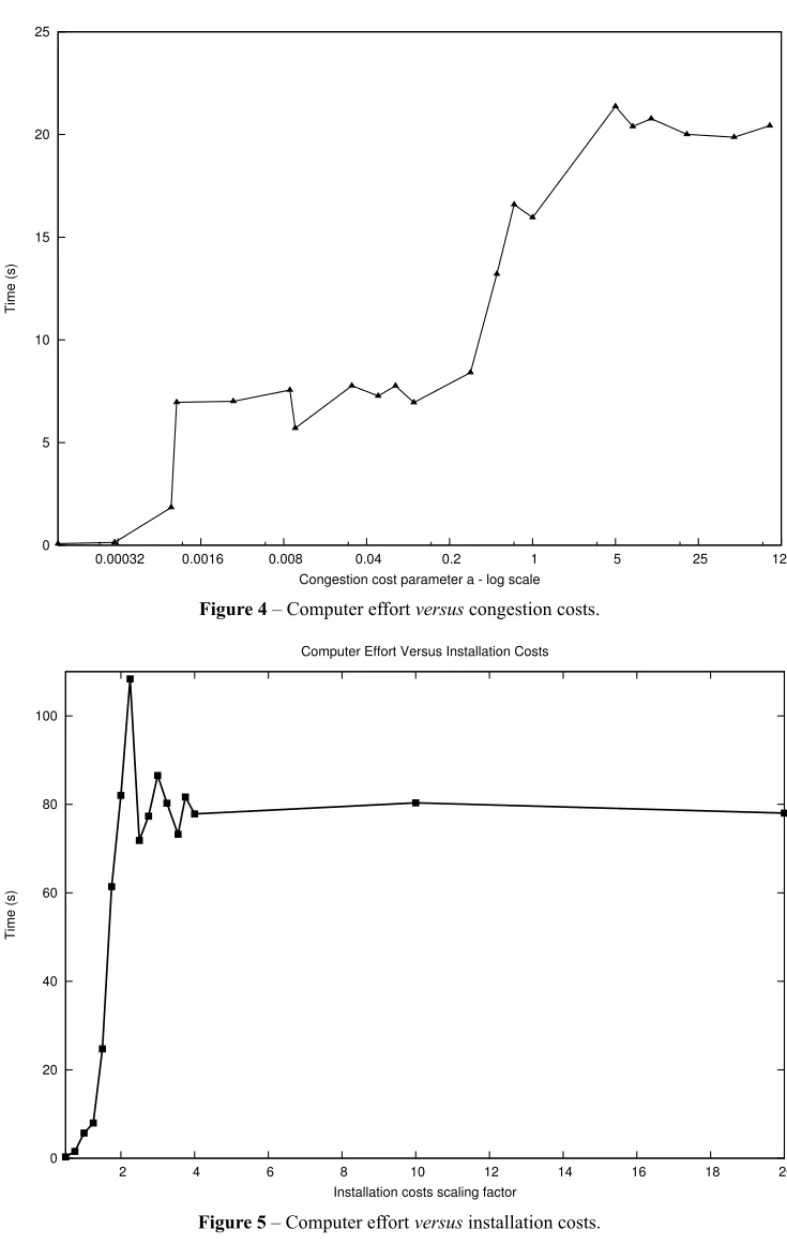
This can be seen in Figure 4 as the computational effort stabilizes after a given threshold of the parameterais trespassed. In other words, all the economies of scale were preserved, at the cost of an additional investment on the network infrastructure.
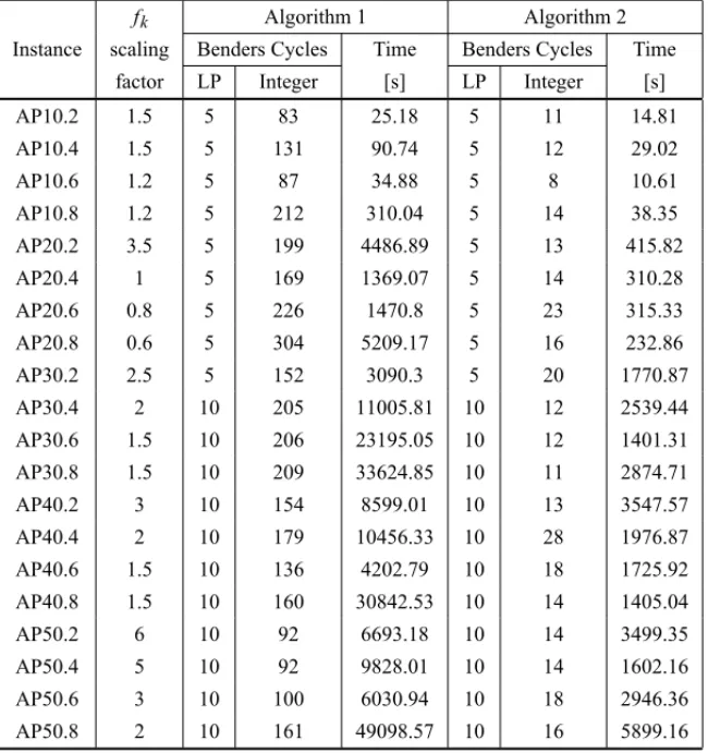
This phenomenon suggests that this class of problems has its inherent difficulty associated to other components than the congestion cost parameters, such as the hub installation costs. In order to investigate the role of these costs, the same instance AP10.2 was used, but having the parametersaandbfixed to 0.001 and 2, respectively. A scaling factor multiplying the installation costs was adopted ranging from 0.5 to 20.
As happened in the later case, Figure 5 shows that after a given threshold of the increased hub installation costs, the computing time to prove the instance optimality is stabilized. Hence from Figures 4 and 5, is possible to infer that the problem under study becomes harder to solve if a given instance presents high hub installation costs and also a very aggressive congestion cost function.
Figure 4– Computer effortversuscongestion costs.
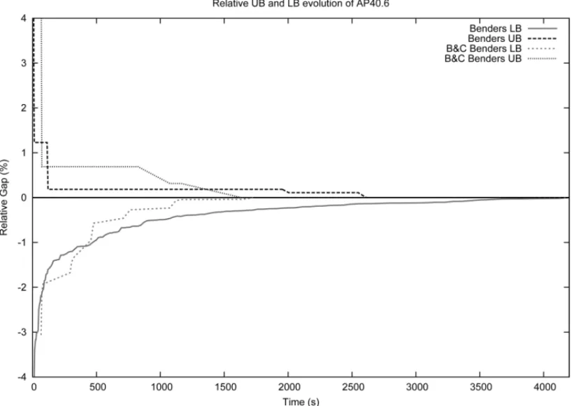
Algorithm 1 requires 7 times more computing time and 11 times more integer cycles than Algo-rithm 2, on average. It is also interesting to remark that there are computing times in Table 2 that are comparable to the ones associated with instances of 150 and 200 nodes of Table 1. Definitely indicating that the complexity of this problem it is not only a matter of instance size.
Table 2– Algorithm 1versusAlgorithm 2.
fk Algorithm 1 Algorithm 2
Instance scaling Benders Cycles Time Benders Cycles Time
factor LP Integer [s] LP Integer [s]
AP10.2 1.5 5 83 25.18 5 11 14.81
AP10.4 1.5 5 131 90.74 5 12 29.02
AP10.6 1.2 5 87 34.88 5 8 10.61
AP10.8 1.2 5 212 310.04 5 14 38.35
AP20.2 3.5 5 199 4486.89 5 13 415.82
AP20.4 1 5 169 1369.07 5 14 310.28
AP20.6 0.8 5 226 1470.8 5 23 315.33
AP20.8 0.6 5 304 5209.17 5 16 232.86
AP30.2 2.5 5 152 3090.3 5 20 1770.87
AP30.4 2 10 205 11005.81 10 12 2539.44
AP30.6 1.5 10 206 23195.05 10 12 1401.31
AP30.8 1.5 10 209 33624.85 10 11 2874.71
AP40.2 3 10 154 8599.01 10 13 3547.57
AP40.4 2 10 179 10456.33 10 28 1976.87
AP40.6 1.5 10 136 4202.79 10 18 1725.92
AP40.8 1.5 10 160 30842.53 10 14 1405.04
AP50.2 6 10 92 6693.18 10 14 3499.35
AP50.4 5 10 92 9828.01 10 14 1602.16
AP50.6 3 10 100 6030.94 10 18 2946.36
AP50.8 2 10 161 49098.57 10 16 5899.16
Furthermore, after observing the evolution of the upper and lower bounds of both algorithms during the solution process of instance AP40.6 of Table 2 (refer to Figure 6), the main advantage of Algorithm 2 over Algorithm 1 is its ability to reduce the tail-off effect. In order to close 1% of optimality gap, Algorithm 2 takes close to a 1000 seconds or 42% of the total time, against 3,600 seconds or 87% of Algorithm 1. An akin behavior occurs on all the other instances.
Figure 6– Convergence curve for Algorithms 1 and 2.
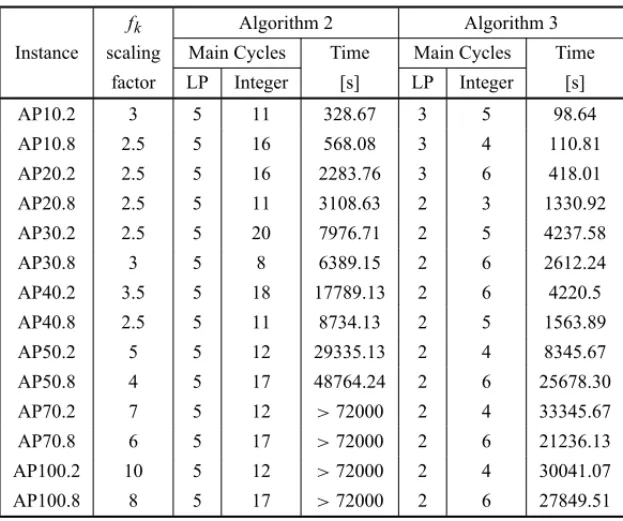
In these final experiments, the congestion cost parameter is set to 0.01 and the installation cost scaling factors were adopted, as indicated in the second column of Table 3. Recall that in the first two sets of experiments, parameterawas set to 0.0001 and 0.001, respectively. In other words, the combined effect of having high congestion and installation costs makes these instances even harder to solve.
Table 3 presents the comparison results of Algorithms 2 and 3. The Algorithm 3 or the OA tech-nique demonstrates a superior performance on these very hard instances, being 3.3 times faster and taking 3 times less integer cycles on average to prove optimality than the Algorithm 3. Notice that Algorithm 2 fails to prove optimality in four instances, ending with an average optimality gap close to 1% (instances AP70 and AP100).
Although, on one hand, Algorithm 3 demonstrates a remarkable performance tackling hard in-stances, on the other hand, the solution effort for solving each OA MP is still very high, even after projecting thexvariables out to reduce its dimension. In this sense, this technique is preferable only if large optimality gaps of the first integer cycles of Algorithm 2 are detected as can be seen in Table 4.
Table 3– Algorithm 2versusAlgorithm 3.
fk Algorithm 2 Algorithm 3
Instance scaling Main Cycles Time Main Cycles Time
factor LP Integer [s] LP Integer [s]
AP10.2 3 5 11 328.67 3 5 98.64
AP10.8 2.5 5 16 568.08 3 4 110.81
AP20.2 2.5 5 16 2283.76 3 6 418.01
AP20.8 2.5 5 11 3108.63 2 3 1330.92
AP30.2 2.5 5 20 7976.71 2 5 4237.58
AP30.8 3 5 8 6389.15 2 6 2612.24
AP40.2 3.5 5 18 17789.13 2 6 4220.5
AP40.8 2.5 5 11 8734.13 2 5 1563.89
AP50.2 5 5 12 29335.13 2 4 8345.67
AP50.8 4 5 17 48764.24 2 6 25678.30
AP70.2 7 5 12 >72000 2 4 33345.67
AP70.8 6 5 17 >72000 2 6 21236.13
AP100.2 10 5 12 >72000 2 4 30041.07
AP100.8 8 5 17 >72000 2 6 27849.51
the hub installation scaling factor and congestion parameteravaried according to the second and third columns, respectively.
The boldfaced entries in Table 4 represents the minimum computational effort for the instances solved. The deployment of Algorithm 3 is more interesting than the others when the optimality gaps of the first integer cycles of Algorithms 1 and 2 are greater than 40% on average for the tested problems.
A final comment is made here necessary. For the authors knowledge, there is no report on the literature that OA methods are able to solve such large scale problems. Notice that the in-stances AP100.2 and AP100.8 have 10,000 integer variables and 49,500,000 continuous vari-ables. Therefore, solving the OA master programs by using the Benders decomposition method is a promising technique,i.e. whenever the problem structure is amenable and the GBD is not a good alternative.
7 FINAL REMARKS
Addressing congestion effects by explicitly considering them as costs on the objective function yields a more realistic modeling approach, specially when suitable nonlinear functions are se-lected. Once the rapid growth of the congestion costs is portrayed, a flow load balancing over the installed infrastructure is induced, leading thus to a superior network design.
Table 4– A direct comparison of the three implemented algorithms.
Instance
Instance Parameters Algorithm 1 Algorithm 2 Algorithm 3 Initial
fk congestion Time Time Time optimality
scaling factor parametera [s] [s] [s] gap [%]
1.00 0.0001 6.98 10.19 11.19 8.17
1.00 0.0005 7.34 9.03 10.70 11.31
1.00 0.0010 6.19 3.14 5.15 26.42
AP10.2 1.00 0.0050 11.26 5.69 6.48 18.73
2.00 0.0010 38.27 15.01 8.22 54.02
2.00 0.0100 84.77 59.19 11.95 73.02
3.00 0.1000 249.59 195.94 86.71 86.15
1.00 0.0001 10.91 14.39 20.48 5.12
1.00 0.0005 57.15 33.99 50.90 19.03
1.00 0.0010 1199.79 293.38 566.50 33.07
AP20.4 1.00 0.0050 1429.65 376.77 569.71 43.05
2.00 0.0010 46474.47 1393.10 303.96 59.93
2.00 0.0100 >72000 24286.90 2267.52 78.84
3.00 0.1000 >72000 >72000 43747.74 85.23
are capable of solving instances up to 100 nodes, being the GBD (Algorithm 1) able to manage larger instances of 150 and 200 nodes.
Finally, the complexity on this class of problems is not only associated with the size of the instances. When an aggressive congestion cost function and large hub installation costs are com-bined, the computational effort to solve these instances may become remarkable. In these cases, the addition of pareto-optimal cuts on the MP branch-and-bound tree is an interesting way to reduce the tail-off effect, improving the overall performance of both of the portrayed methods: GBD and OA. In general, on one hand the GBD method is more scalable with instance size, on the other hand, the OA technique is less affected by the tail-off effect.
ACKNOWLEDGMENTS
The authors’ research has been funded by Conselho Nacional de Pesquisa – CNPq, project 480757/2008-9.
REFERENCES
[1] ABDINNOUR-HELM S. 1998. A hybrid heuristic for the uncapacitated hub location problem. European Journal of Operational Research,2-3(106): 489–499.
[3] ABDINNOUR-HELM S & VENKATARAMANAN MA. 1998. Solution approaches to hub location problems.Annals of Operations Research,78: 31–50.
[4] ADJIMANCS, ANDROULAKISIP & FLOUDASCA. 1997. Global optimization of MINLP problems in process synthesis and design.Computers & Chemical Engineering,21(Suppl. S): S445–S450. [5] ALUMUR SA & KARABY. 2008. Network hub location problems: The state of the art.European
Journal of Operational Research,190: 1–21.
[6] ALUMURSA, KARABY & KARASANOE. 2009. The design of single allocation incomplete hub networks.Transportation Research Part B,43: 936–951.
[7] AYKIN T. 1994. Lagrangian relaxation based approaches to capacitated hub-and-spoke network design problem.European Journal of Operational Research,79: 501–523.
[8] AYKINT. 1995. Network policies for hub-and-spoke systems with applications to the air transporta-tion system.Transportation Science,29: 201–221.
[9] BENDERS JF. 1962. Partitioning procedures for solving mixed-variables programming problems. Numerisch Mathematik,4: 238–252.
[10] CAMARGORS, MIRANDAJRGDE& LUNAHP. 2008. Benders decomposition for the uncapaci-tated multiple allocation hub location problem.Computers and Operations Research,35: 1047–1064. [11] CAMARGORS, MIRANDAJRGDE, FERREIRAR & LUNAHP. 2009. Multiple allocation hub-and-spoke network design under hub congestion.Computers and Operations Research,36: 3097–3106. [12] CAMARGORS, MIRANDAJR GDE & LUNAHP. 2009. Benders decomposition for hub location
problems with economies of scale.Transportation Science,43: 86–97.
[13] CAMARGO RS, MIRANDA JR G DE & FERREIRA RPM. 2011. A hybrid outer-approximation/ benders decomposition algorithm for the single allocation hub location problem under congestion. Operations Research Letters,39(5): 329–337.
[14] CAMPBELLJF. 1994. Integer programming formulations of discrete hub location problems. Euro-pean Journal of Operational Research,72: 387–405.
[15] CAMPBELLJF. 1994. A survey of network hub location.Studies in Locational Analysis,6: 31–49. [16] CAMPBELLJF, ERNSTAT & KRISHNAMOORTHYM. 2002. Hub location problems. In: Drezner Z
and Hamacher HW (editors), Facility Location: Applications and Theory, chapter 12, pages 373–407. Springer, 1stedition.
[17] CHEN JF. 2007. A hybrid heuristic for the uncapacitated single allocation hub location problem. Omega,35: 211–220.
[18] CONTRERASI, FERNANDEZ E & MARN A. 2010. The tree of hubs location problem.European Journal of Operational Research,202: 390–400.
[19] CORDEAUJF, SOUMISF & DESROSIERSJ. 2001. Simultaneous assignment of locomotives and cars to passenger trains.Operations Research,49(4): 531–548.
[20] COSTAMDAG, CAPTIVO ME & CL´IMACOJ. 2008. Capacitated single allocation hub location problema bi-criteria approach.Computers and Operations Research,35(11): 3671–3695.
[21] CUNHACB & SILVA MR. 2007. A genetic algorithm for the problem of configuring a hub-and-spoke network for a LTL trucking company in Brazil.European Journal of Operational Research,
![Figure 3 – Computer burden trend (log(Time[s])).](https://thumb-eu.123doks.com/thumbv2/123dok_br/18870838.420047/24.1063.119.882.160.734/figure-computer-burden-trend-log-time-s.webp)