Integrated statistical modelling of spatial landslide probability

(1)

NHESSD

3, 5677–5715, 2015

Integrated statistical modelling of spatial landslide probability

M. Mergili and H.-J. Chu

Title Page

Abstract Introduction

Conclusions References

Tables Figures

◭ ◮

Back Close

Full Screen / Esc

Printer-friendly Version Interactive Discussion

Discussion

P

a

per

|

Discussion

P

a

per

|

Discussion

P

a

per

|

Discussion

P

a

per

|

Nat. Hazards Earth Syst. Sci. Discuss., 3, 5677–5715, 2015 www.nat-hazards-earth-syst-sci-discuss.net/3/5677/2015/ doi:10.5194/nhessd-3-5677-2015

This discussion paper is/has been under review for the journal Natural Hazards and Earth System Sciences (NHESS). Please refer to the corresponding final paper in NHESS if available.

Integrated statistical modelling of spatial

landslide probability

M. Mergili1,2and H.-J. Chu3

1

Geomorphological Systems and Risk Research, Department of Geography and Regional Research, University of Vienna, Universitätsstraße 7, 1190 Vienna, Austria

2

Institute of Applied Geology, University of Natural Resources and Life Sciences (BOKU), Peter-Jordan-Straße 70, 1190 Vienna, Austria

3

Department of Geomatics, National Cheng Kung University, 1 University Road, 701 Tainan, Taiwan

Received: 26 August 2015 – Accepted: 3 September 2015 – Published: 24 September 2015

Correspondence to: M. Mergili ([email protected])

(2)

NHESSD

3, 5677–5715, 2015

Title Page

Tables Figures

◭ ◮

Back Close

Full Screen / Esc

Discussion

P

a

per

|

Discussion

P

a

per

|

Discussion

P

a

per

|

Discussion

P

a

per

|

Abstract

Statistical methods are commonly employed to estimate spatial probabilities of land-slide release at the catchment or regional scale. Travel distances and impact areas are often computed by means of conceptual mass point models. The present work intro-duces a fully automated procedure extending and combining both concepts to compute

5

an integrated spatial landslide probability: (i) the landslide inventory is subset into re-lease and deposition zones. (ii) We employ a simple statistical approach to estimate the pixel-based landslide release probability. (iii) We use the cumulative probability density function of the angle of reach of the observed landslide pixels to assign an impact probability to each pixel. (iv) We introduce the zonal probability i.e. the spatial

proba-10

bility that at least one landslide pixel occurs within a zone of defined size. We quantify this relationship by a set of empirical curves. (v) The integrated spatial landslide prob-ability is defined as the maximum of the release probprob-ability and the product of the impact probability and the zonal release probability relevant for each pixel. We demon-strate the approach with a 637 km2study area in southern Taiwan, using an inventory

15

of 1399 landslides triggered by the typhoon Morakot in 2009. We observe that (i) the average integrated spatial landslide probability over the entire study area corresponds reasonably well to the fraction of the observed landside area; (ii) the model performs moderately well in predicting the observed spatial landslide distribution; (iii) the size of the release zone (or any other zone of spatial aggregation) influences the integrated

20

spatial landslide probability to a much higher degree than the pixel-based release prob-ability; (iv) removing the largest landslides from the analysis leads to an enhanced model performance.

(3)

NHESSD

3, 5677–5715, 2015

Title Page

Tables Figures

◭ ◮

Back Close

Full Screen / Esc

Discussion

P

a

per

|

Discussion

P

a

per

|

Discussion

P

a

per

|

Discussion

P

a

per

|

1 Introduction

Overviews of spatial landslide probability (susceptibility) at catchment or regional scales are useful for hazard indication zoning and for prioritizing target areas for risk mitigation. Computer models making use of geographic Information Systems (GIS) are commonly employed to produce such overviews (Van Westen et al., 2006).

Physically-5

based modelling of landslide susceptibility – also with reasonably complex modelling tools – has become an option also for large areas from a purely technical point of view (Mergili et al., 2014a, b). However, the parameterization of such models remains a chal-lenge, limiting the quality of the results obtained. For this reason, statistical methods – often coupled with stochastic concepts – are commonly employed to relate the spatial

10

patterns of landslide occurrence to those of environmental variables, and to estimate landslide susceptibility by applying these relationships (Guzzetti, 2006). A broad array of statistical methods for landslide susceptibility analysis has been developed, docu-mented by a large bunch of publications (e.g. Carrara et al., 1991; Baeza and Coromi-nas, 2001; Dai et al., 2001; Lee and Min, 2001; Brenning, 2005; Saha et al., 2005;

15

Guzzetti, 2006; Komac, 2006; Lee and Sambath, 2006; Lee and Pradhan, 2007; Yal-cin, 2008; Yilmaz, 2009; Nandi and Shakoor, 2010; Yalcin et al., 2011; Petschko et al., 2014). However, such methods only concern the release of landslides whilst they dis-regard their propagation.

Whilst advanced physically-based models for landslide propagation (e.g.

Chris-20

ten et al., 2010a, b) are usually employed for local-scale studies, conceptual ap-proaches have been developed to analyze and to estimate travel distances and im-pact areas at broader scales. Some build on the angle of reach or related parameters (e.g. Scheidegger (1973) for rock avalanches; Zimmermann et al. (1997) and Ricken-mann (1999) for debris flows; Corominas et al. (2003) for various types of landslides;

25

(4)

pre-NHESSD

3, 5677–5715, 2015

Title Page

Tables Figures

◭ ◮

Back Close

Full Screen / Esc

Discussion

P

a

per

|

Discussion

P

a

per

|

Discussion

P

a

per

|

Discussion

P

a

per

|

sented an automated approach to statistically derive cumulative density functions of the angle of reach from a given landslide inventory, and to apply these functions to com-pute a spatially distributed impact probability. Modelling approaches considering both the release and the propagation of landslides do exist (Mergili et al. (2012) and Hor-ton et al. (2013) for debris flows; Gruber and Mergili (2013) for various high-mountain

5

processes). However, they yield deterministic results distinguishing areas with an im-pact expected from those with no imim-pact expected, or qualitative scores.

Integrated automated approaches to properly estimate the spatial probability of a given area to be affected by a landslide – considering both release and propaga-tion – are still missing. The present work attempts to fill this gap by combining the two

10

newly developed open source software tools r.landslides.statistics and r.randomwalk. We will next introduce our modelling strategy (Sect. 2) and the study area in Taiwan (Sect. 3). After presenting (Sect. 4) and discussing (Sect. 5) the results we will conclude with a set of key messages (Sect. 6).

Within the present article we use the term “landslide” in a broad sense, including all

15

relevant types of gravitational mass movements.

2 Modelling strategy

2.1 General model layout

We propose an integrated statistical procedure (containing stochastic elements) to compute the spatial probability of a given area (technically, a given GIS pixel) to be

20

affected by a landslide either through its release or through its propagation. We first consider release and propagation separately and finally combine the two concepts. The entire work flow is illustrated in Fig. 1, its components are introduced in detail in Sects. 2.2–2.6.

Two newly developed raster modules of the open source software package GRASS

25

GIS 7 (Neteler and Mitasova, 2007; GRASS Development Team, 2015) are combined:

(5)

NHESSD

3, 5677–5715, 2015

Title Page

Tables Figures

◭ ◮

Back Close

Full Screen / Esc

Discussion

P

a

per

|

Discussion

P

a

per

|

Discussion

P

a

per

|

Discussion

P

a

per

|

– r.landslides.statistics allows inventory subsetting, estimation of the spatial proba-bility of landslide release, and the generation of a zonal probaproba-bility function.

– r.randomwalk, introduced by Mergili et al. (2015), employs sets of constrained random walks to route hypothetic mass points down through the digital eleva-tion model (DEM) and assigns an impact probability to each pixel. The

cumula-5

tive probability density function (CDF) used is derived from the analysis of the observed landslides. Further, r.randomwalk includes an algorithm to combine re-lease probabilities and impact probabilities, making use of the zonal probability function derived with r.landslides.statistics.

Both tools build on a combination of the Python and C programming languages. The

10

R software environment for statistical computing and graphics (R Core Team, 2015) is used for built-in validation and visualization functions. r.landslides.statistics and r.randomwalk can be started in a fully non-interactive way i.e. all parameters are passed as command line arguments. This strategy enables a straightforward combination of multiple runs of the two models at the script level.

15

An issue of central importance consists in the strict separation of the data used for model development and the data used for model application and evaluation. In this sense, most operations are performed either for the model development area (MDA) or for the model evaluation area (MEA), but not for both. The only exception from this rule applies to the initial step of inventory subsetting.

20

All probabilities used in the context of the present work are summarized in Table 1.

2.2 Inventory subsetting

Landslide inventories often suffer from a missing – or unsatisfactory – subsetting into release, transit and deposition areas. The reason for this problem, which applies also to our case study, is not necessarily related to deficient mapping efforts, but rather to the

25

(6)

NHESSD

3, 5677–5715, 2015

Title Page

Tables Figures

◭ ◮

Back Close

Full Screen / Esc

Discussion

P

a

per

|

Discussion

P

a

per

|

Discussion

P

a

per

|

Discussion

P

a

per

|

landslide release or propagation. We therefore suggest a reproducible procedure to deal with this problem.

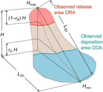
We analyze the geometric properties of all landslides in a given inventory in terms of inclination, minimum and maximum elevation, elevation range, central, maximum and average 2-D and 3-D length and width, 2-D and 3-D areas. Lengths and widths are

5

defined as Euclidean distances (the central 2-D and 3-D lengthsL2-DandL3-Das well

as the elevation range H are shown in Fig. 2). On this basis we compute the height ratiorH for each observed landslide pixel:

rH=

Hp−Hmin

Hmax−Hmin

, (1)

whereHpis the elevation at the considered pixel,Hmin is the minimum elevation of the

10

landslide andHmaxis the maximum elevation of the landslide (see Fig. 2).

In the present work, we consider all observed landslide pixels withrH≥rRas release

pixels and all observed landslide pixels withrH≤rDas deposition pixels.rRandrDare

defined by the user. All other observed landslide pixels are considered as unknowns regarding release and deposition. Following these rules, we obtain three landslide

in-15

ventory maps:

1. observed release areas (ORA), where all release pixels are considered observed positives (OP), the rest of the landslide areas are considered no data, and all non-landslide pixels are considered observed negatives (ON);

2. observed deposition areas (ODA), where all deposition pixels are considered OP,

20

the rest of the landslide areas are considered no data, and all non-landslide pixels are considered ON;

3. observed impact areas (OIA), where all landslide pixels are considered OP, and all non-landslide pixels are considered ON.

These definitions prevent us from including pixels in the statistical analysis and the

25

(7)

NHESSD

3, 5677–5715, 2015

Title Page

Tables Figures

◭ ◮

Back Close

Full Screen / Esc

Discussion

P

a

per

|

Discussion

P

a

per

|

Discussion

P

a

per

|

Discussion

P

a

per

|

excuding all uncertain pixels we have to chose conservative values ofrR and rD,

re-sulting in a decreased number of OP pixels used for the statistical analyses and their validation.

2.3 Pixel-based release probability

Statistical analyses of landslide spatial release probability (landslide susceptibility)

5

have been treated exhaustively in previous studies (see Sect. 1 for references). In the context of the present work we are bound to a method yielding spatial probabilities in the range 0–1. In this sense, we employ a simple approach building on the spa-tial overlay of classified predictor maps. Considering separately each of the resulting combinations of predictor classes, we compute the fractionfR of observed landslide

10

release pixels related to all pixels. For this step we consider only the MDA. Building on the assumption that possible future landslides in the MEA are spatially related to the predictors in the same way as the observed landslides in the MDA, the release proba-bilityP_R (see Table 1) for each pixel in the MEA is set to the value off_Rassociated to the corresponding combination of predictor classes.

15

The true positive (TP), true negative (TN), false positive (FP) and false negative (FN) pixel counts are derived for selected levels ofP_R. An ROC Curve is produced by plotting the true positive rate TP/OP against the false positive rate FP/ON.

2.4 Zonal release probability

It is useful for many purposes to work with pixel-based spatial release probabilities

20

(P_R). They can be averaged in order to characterize the spatial probability of landslides for any type of zone (such as slope units, catchment basins, administrative entities or larger pixels). However, the average of PR over a certain zone does not tell us how

likely it is that a landslide occurs in a zone at all. For this purpose we introduce the zonal release probabilityPRZ(see Table 1) which increases with study area size. When

25

(8)

NHESSD

3, 5677–5715, 2015

Title Page

Tables Figures

◭ ◮

Back Close

Full Screen / Esc

Discussion

P

a

per

|

Discussion

P

a

per

|

Discussion

P

a

per

|

Discussion

P

a

per

|

entire countries)PRZ=1 as there will always be at least one landslide pixel.PRZ may

be useful for assessing how likely it is that a certain object (such as a road) is affected by a landslide at all. It is further the appropriate parameter when validating landslide probability at the level of slope units or other entities larger than single pixels. In the present work it is needed primarily as a basis to compute the integrated spatial

land-5

slide probabilityPL (see Sect. 2.6). It is further used to aggregate the model results at

the level of slope units.

PRZ cannot be computed in a fully analytic way. We suggest an empirical approach

to approximatePRZ(Fig. 3):

1. a subset of the MDA with a randomized size and randomized centre coordinates is

10

selected. P_RO is the observed pixel-based spatial probability of landslide release in this subset (i.e. the fraction of ORA pixels out of all pixels);

2. within this subset, a set of sub-subsets with constant zone sizeZand randomized centre coordinates is tested for the presence of observed landslide release pixels. The observed zonal release probabilityPRZO is defined as the fraction of subsets

15

with at least one observed landslide release pixel (see Fig. 3a);

3. (2) is repeated for a large number of sets of sub-subsets covering a broad range ofZ.

(1)–(3) are repeated for a large number of random subsets of the MDA.

This procedure results in a line cloud of PRZO plotted againstZ (one line for each

20

subset; Fig. 3b). A logistic regression is fitted to the average value ofPRZO,µPRZO, for

each tested value ofZ:

µ_PRZO(Z)= (1−µPRO)

1+e−(a₂+a₃Z)+µPRO, (2)

wherea2anda3are the regression coefficients andµPROis the fraction of the observed

landslide area within the considered zone. We will come back to the function introduced

25

in Eq. (2) in Sect. 2.6.

(9)

NHESSD

3, 5677–5715, 2015

Title Page

Tables Figures

◭ ◮

Back Close

Full Screen / Esc

Discussion

P

a

per

|

Discussion

P

a

per

|

Discussion

P

a

per

|

Discussion

P

a

per

|

2.5 Impact probability

The tool r.randomwalk (Mergili et al., 2015) is employed for routing mass points rep-resenting hypothetic landslides through the DEM. The specific impact probability PIR

describes the probability of an arbitrary impact pixel to be hit by a mass point routed from a defined release pixel through the DEM. The impact probabilityP∗

I orPI results

5

from the spatial overlay of all relevant values of PIR at a certain pixel (see Table 1).

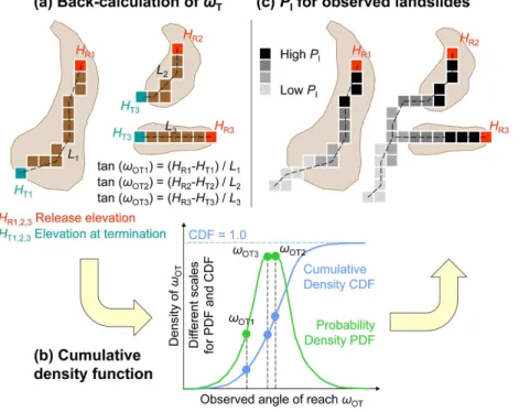
We definePIR on the basis of the angle of the path ωbetween the release pixel and

a possible impact pixel. This approach follows the concept of the angle of reach (Heim, 1932; Fig. 4).PI is computed in three steps:

1. The CDF describing the probability that a moving mass point starting from an

10

arbitrary release pixel leaves the OIA of the same landslide at or below a cer-tain threshold of ωis derived for the MDA. This is done by back-calculating the observed angles of reachωOT for all observed landslides (see Fig. 4a) and

ana-lyzing the resulting probability density (see Fig. 4b).

2. The CDF is then employed to compute PIR with regard to all observed release

15

pixels in the MEA and evaluated against the ODA by means of an ROC Plot (see Sect. 2.3). For those pixels with impacts from more than one release pixel, P_I∗ takes the maximum value out of all relevant values ofPIR(see Fig. 4c).

3. The same CDF is used for computingPIRwith regard to all pixels in the MEA. For

reasons to be explained in Sect. 2.6, for those pixels with impacts from more than

20

one release pixelPI takes the average value of all relevant values ofPIR.

2.6 Integrated spatial landslide probability

The integrated spatial landslide probabilityPLapproximates the spatial probability that

a landslide coincides spatially with an arbitrary pixel of the MEA, either through its release or through its impact (see Table 1). In principle,PL is computed by multiplying

(10)

NHESSD

3, 5677–5715, 2015

Title Page

Tables Figures

◭ ◮

Back Close

Full Screen / Esc

Discussion

P

a

per

|

Discussion

P

a

per

|

Discussion

P

a

per

|

Discussion

P

a

per

|

a release probability and an impact probability. Obviously, a simple overlay ofPR and

PI would be useless. Instead, we have to consider for each impact pixel withPI>0 the

zonal release probabilityPRZof the possible release zone (Fig. 5) relevant for this pixel.

Z and the associated value of µPR (see Sect. 2.4) refer to the entire set of release

pixels which may propagate all the way to the impact pixel. I.e.PRZhas to be computed

5

separately for each impact pixel.

For this purpose, we come back to the function introduced in Eq. (2). Thereby we assume that the shape of the logistic regression function is insensitive to the zonal average of the computed values ofPR,µPR, of any arbitrary subset of the study area

with zone sizeZ (see Fig. 3c):

10

1−P_RZ(Z)

1−µ_PRZO(Z)

∼ 1−µPR

1−µ_PRO. (3)

Reformulating Eq. (3),PRZ(Z) is computed as

PRZ(Z)∼1−(1−µPRZO(Z))

1−µ_PR

1−µ_PRO. (4)

For those pixels wherePRZ·PI< PR,PLis set toPR. For all other pixels,PLis set to the

product ofPRZandPI:

15

PL=max(PR,PRZ·PI). (5)

The resulting raster map ofPL is evaluated against the OIA by means of an ROC Plot

(see Sect. 2.3).

The expected error of PRZ is explored by comparing the empirical values of PRZO

obtained for each subset and each zone size with the results of Eq. (2) (see Fig. 3d). It

20

is expressed as a third-order polynomial regression function of the standard deviation ofPRZ:

σPRZ=b1+b2log10Z+b3(log10Z)2+b4(log10Z)3, (6)

(11)

NHESSD

3, 5677–5715, 2015

Title Page

Tables Figures

◭ ◮

Back Close

Full Screen / Esc

Discussion

P

a

per

|

Discussion

P

a

per

|

Discussion

P

a

per

|

Discussion

P

a

per

|

whereσPRZis the standard deviation ofPRZandb1–b4are the regression coefficients.

The standard deviation ofPL,σPL, is derived as

σPL=σPRZ·PI. (7)

Equation (7) only applies to those pixels wherePRZ·PI≥PR.

We note that the described procedure is supposed to yield smoothed results due

5

to averaging effects: (i) Eq. (5) builds on the simplification of a uniformly distributed release probability over the possible release zone. (ii) As highlighted in Sect. 2.5, PI

represents the average ofPIRof all mass points impacting a pixel. This type of

averag-ing is necessary to ensure a consistent combination ofPRZandPI.

3 Test area and parameterization 10

3.1 The Kao Ping test area

In the period from 7 to 9 August 2009, Typhoon Morakot triggered a high number of landslides in Taiwan. According to Lin et al. (2011), more than 22 000 landslides were recorded in Southern Taiwan. One of the hot spots was the Kao Ping Watershed (Wu et al., 2011), where extremely heavy rainfall (more than 2000 mm in a period of

15

90 h) caused an enormous amount of mass wasting and triggered a catastrophic land-slide in the Hsiaolin Village (Kuo et al., 2013).

We consider a 637 km2 subset of the Kao Ping Watershed for computing the in-tegrated spatial landslide probabilityPL (Fig. 6). 1399 landslides triggered by the

Ty-phoon Morakot are mapped in the shale, sandstone and colluvium slopes of the area.

20

A stereo-photogrammetrically generated 10 m DEM is used along with a landslide in-ventory derived from FORMOSAT-2 scenes recorded before and after the event. The landslide inventory delineates the OIA without differentiating between ORA and ODA, and without providing direct information on landslide volumes. Overlapping landslide polygons are aggregated to one polygon for the purpose of the statistical analyses.

(12)

NHESSD

3, 5677–5715, 2015

Title Page

Tables Figures

◭ ◮

Back Close

Full Screen / Esc

Discussion

P

a

per

|

Discussion

P

a

per

|

Discussion

P

a

per

|

Discussion

P

a

per

|

3.2 Model parameterization

The model tests are summarized in Table 2. The Kao Ping study area is divided into four subsets (A–D in Fig. 6) to separate between MDA and MEA. In each of the tests, three subsets are used as MDA and one subset is used as MEA. The division lines between the subsets follow catchment boundaries in order to ensure that all landslides

5

are clearly assigned to one of the four subsets and no landslide may impact more than one subset. All tests are run at a pixel size of 20 m.

We use values of rR=0.75 and rD=0.25 (see Sect. 2.2). Preliminary tests have

shown that the following two parameters are suitable as predictors for computingPR:

(i) local slope (five classes); and (ii) aspect (2 classes). For reasons of the regional

10

geology, NE–E–SE–S–SW exposed slopes are more affected by landslides than W– NW–N exposed slopes. Both predictors are derived from a modified version of the DEM: noise reduction is applied to the DEM through a low pass filter building on the mean of all values within in a radius of 50 m.

For back-calculatingωOT and for evaluatingP

∗

I we start a set of 10 3

random walks

15

from each pixel in the ORA of the MDA and the MEA, respectively. For computingPL

we start a set of 102 random walks from each pixel in the MEA. We use Gaussian distributions to generate the CDFs. The input parameters governing the routing pro-cedure in r.randomwalk are chosen in accordance with the suggestions provided by Mergili et al. (2015).

20

Preliminary tests have further indicated that the largest, deep-seated landslides in the test area are poorly predicted by the statistical model applied. We hypothesize that landsides of this type are governed by other factors than those which can be derived directly from the DEM or other surface data. The analyses are therefore repeated ex-cluding all landslides with a total size of the OIA≥1 km2. All pixels within the OIA of

25

those landslides are set to no data (Tests 2A–D in Table 2).

We further run the model with a spatially constant value of PR (identical to the

ob-served density of ORA in the MDA) in order to quantify the component ofPL(and of the

(13)

NHESSD

3, 5677–5715, 2015

Title Page

Tables Figures

◭ ◮

Back Close

Full Screen / Esc

Discussion

P

a

per

|

Discussion

P

a

per

|

Discussion

P

a

per

|

Discussion

P

a

per

|

model performance) associated to the zone size used for computingPRZ(see Sect. 2.6;

Tests 3A–D in Table 2).

The model results are evaluated against the observed landslides at two spatial levels using ROC Plots:

– The pixel level.PRis evaluated against the ORA,P

∗

I is evaluated against the ODA,

5

andPLis evaluated against the OIA.

– The level of slope units. The slope units are derived using the GRASS GIS module r.watershed (parameter half_basin), with a minimum area of one slope unit of 104m2. Each slope unit with at least one OP pixel is considered OP. The average and zonal values ofPRandPLas well as the slope unit size are tested against the

10

corresponding aggregated inventories.

4 Results

4.1 Spatial patterns of landslide probability

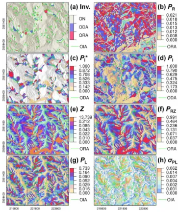
Figure 7 illustrates the result maps for test 1C. For reasons of clarity, we show only a subset of the test area (see Fig. 6). However, the general patterns of the results are

15

well represented in this area and are also valid for the other tests. Figure 7a shows the result of the inventory subsetting, the spatial variation ofPRis displayed in Fig. 7b.

Whilst the patterns ofP∗

I related to the observed landslide release pixels (see Fig. 7c)

clearly reflect the decreasing probabilities in downslope direction, the values ofPI

re-lated to all possible release pixels (see Fig. 7c) are high where large contiguous steep

20

slopes are present i.e. where the average slope angles are high. The probability den-sity function and the CDF ofωOT computed for the relevant MDA (including the zones

A, B and D; see Fig. 6) are shown in Fig. 8a. According to the Figs. 4 and 8a,P∗

I =1 for

(14)

NHESSD

3, 5677–5715, 2015

Title Page

Tables Figures

◭ ◮

Back Close

Full Screen / Esc

Discussion

P

a

per

|

Discussion

P

a

per

|

Discussion

P

a

per

|

Discussion

P

a

per

|

all mass points possibly impacting the considered pixel asPI represents the average of

all relevant values ofPIR(see Fig. 5)

The largest values ofZ are displayed in those areas with large catchments i.e. in the valleys (see Fig. 7e). Whilst the maxima exceed 10 km2in zone C, the median ofZ for all pixels in zone C is 0.043 km2. The zonal release probability (see Fig. 7f) strongly

5

reflects the patterns ofZ, clearly dominating over the influence ofPR(see Figs. 3 and

7b). This phenomenon is explained by the limited spatial variation ofP_R (see Fig. 7b) and the resulting dominance of the zone size reflected inPRZ. Figure 9a illustrates the

dependency of the observed zonal release probability PRZO from the zone size (see

Fig. 3).

10

Note that high values of PRZ are not associated to those areas with high release

probabilities, but to the source areas of the random walks determining PI of the

cor-responding pixel (see Fig. 5). However,PI is usually low in those areas with very high

values ofPRZas they are located in the valleys at some distance from the steep slopes.

Therefore, the integrated spatial landslide probability PL reaches its maxima on the

15

lower slopes and in narrow gorges, where both PRZ and PI are relatively high (see

Fig. 7g). The standard deviation shown in Fig. 7h is derived from the standard devia-tion funcdevia-tion of Fig. 9b (see Eqs. 6 and 7).σPRZ remains at a moderate level and is

highest in those areas where alsoPRZis high.

Figure 10 shows the distribution ofPLfor the entire test area. The maps for the tests

20

1A–1D – each of them covering the corresponding MEA – are combined into one map.

4.2 Pixel-based evaluation against observed landslides

Considering all observed landslides (tests 1A–D), 7.5 % of the entire test area are clas-sified as OIA (i.e. the observed integrated spatial landslide probability). The average value ofPL=9.3 %, meaning that we arrive at a reasonable estimate of the integrated

25

spatial landslide probability, even though we overestimatePL. The same is true for the

landslide release areas, where 1.4 % of the test area are classified as ORA, with a simi-lar average value ofPR. Whilst the excellent correspondence of observed and modelled

(15)

NHESSD

3, 5677–5715, 2015

Title Page

Tables Figures

◭ ◮

Back Close

Full Screen / Esc

Discussion

P

a

per

|

Discussion

P

a

per

|

Discussion

P

a

per

|

Discussion

P

a

per

|

release probabilities is forced by the type of statistical approach employed, the still rea-sonable correspondence with regard toPRindicates a certain validity of the suggested

workflow. The key parameters characterizing the outcomes of each test (see Table 2) are summarized in Table 3. Observed and computed percentages are lower for the tests 2A–D as some landslide areas are removed from the analysis.

5

The ROC Plots for model evaluation are compiled in Fig. 11.PRis evaluated against

the ORA, P_I is evaluated against the ODA and P_L is evaluated against the OIA. Only the MEA is taken into account. Considering the tests 1A–D, the predictors slope and aspect only explain part of the spatial variation ofPR, indicated by moderate levels of

AUC_ROC (0.569–0.661). The prediction level of test 1D even indicates model failure

10

(see Fig. 11a). In contrast, the spatial variation of the observed deposition areas is comparatively well predicted by the modelled values ofP∗

I (0.724≤AUCROC≤0.913;

see Fig. 11b). This observation is not surprising as the possible path of movement is usually reasonably well constrained, and most mass points necessarily touch the observed impact areas whilst those pixels on slopes without observed landslides yield

15

a large amount of “cheap” TN pixels (see Fig. 7c). WhilstPIderived by the routing of all

possible release pixels (see Fig. 7d) is of theoretical nature and would be less useful to evaluate, PL again displays a moderate prediction level (0.605≤AUCROC≤0.685;

see Fig. 11b) which is, however, better than PR. Considering the ROC Plots for PR

andP_I∗ indicates that the false predictions are a consequence of the uncertain release

20

probability rather than of deficiencies in the routing procedure.

Removing the largest landslides (OIA≥1 km2) from the data (Tests 2A–D) does not significantly change the general prediction quality with regard to PR (see Fig. 11d).

However, in the test 2D AUCROC increases from 0.569 to a (still very low) value of

0.598, indicating that the large Hsiaolin Landslide located in zone D (see Fig. 6) is very

25

poorly explained by the predictors used. The influence of removing large landslides (all of which are located in the zones C and D) on the model performance in terms of P∗

I is more obvious than in the case ofPR (see Fig. 11e). The tests 2C and 2D display

(16)

NHESSD

3, 5677–5715, 2015

Title Page

Tables Figures

◭ ◮

Back Close

Full Screen / Esc

Discussion

P

a

per

|

Discussion

P

a

per

|

Discussion

P

a

per

|

Discussion

P

a

per

|

and 0.724 to 0.900, respectively). This phenomenon is again a consequence of the particular settings associated to the large landslides (especially the Hsiaolin Landslide, the deposition area of which is very poorly predicted) yielding a large number of false negative pixels in the observed deposit. Coming back to Fig. 8b, the tests 1A–D yield lower peaks of the probability density and a shift of the curves towards lower values

5

of ωOT, compared to the tests 2A–D (see Table 3). Those lower values of ωOT are

associated to the large landslides excluded in the tests 2A–D. Consequently, ω_T is underestimated – and therefore, the impact area is overestimated – for the majority of the observed landslides in the tests 1A–D. However, the shift in the model performance is related to the poor prediction of the large deposit of the Hsiaolin Landslide rather

10

than to the changes in the CDF.

In accordance with the patterns observed with regard to PI, AUCROC increases for

the tests 2C and D, compared to 1C and D (see Fig. 11f). In contrast, AUCROC forPL

derived with the tests 2A and B decreases slightly, compared to the values obtained with the results for 1A and B. Figure 11g illustrates the ROC Curves yielded for PL,

15

assuming a constant spatial pattern ofPR(i.e. the fraction of observed landslide pixels

in the MEA for each test 3A–D). The values of AUC_ROC are almost similar to those yielded with the tests 1A–D (see Fig. 11c). This observation indicates that the spatial differentiation of PR is almost completely covered by the patterns of PI and Z (see

Fig. 7).

20

4.3 Evaluation against observed landslides on the basis of slope units

The ROC Plots shown in the Fig. 11h–l relate the modelled distribution ofPR and PL

to the distribution of OP and ON slope units of the entire test area (in each case, the combination of the results of the tests A–D). All slope units with at least one OP pixel are considered OP, the ROC Curves are weighted for the slope unit size. The AUCROC

25

values derived for the average values ofPR for each slope unit evaluated against the

aggregated ORA are significantly higher than the AUC_ROC values derived at the pixel level (0.695 for the tests 1A–D and 0.723 for the tests 2A–D; see Fig. 11h and j).

(17)

NHESSD

3, 5677–5715, 2015

Title Page

Tables Figures

◭ ◮

Back Close

Full Screen / Esc

Discussion

P

a

per

|

Discussion

P

a

per

|

Discussion

P

a

per

|

Discussion

P

a

per

|

AUC_ROC further increases to 0.787 and 0.766, respectively, when the zonal values of PR for the slope units are considered. This would be the correct way. However, these

zonal probabilities are extremely strongly correlated to the size of the associated slope unit (this phenomenon is already indicated by Fig. 9), so that validating the zone size against the ORA results in ROC Curves almost identical with those derived for the

5

zonal probabilities. This means that, despite the high values of AUCROC, the zonal

values of P_R for the slope units have no predictive power in terms of differentiating between areas of varying environmental or topographic conditions. The high prediction quality just relies on the fact that larger slope units are more likely to contain OP pixels (see Sect. 2.4). This phenomenon was already indirectly shown by the comparison of

10

the Fig. 11c and g.

Slope units are not the suitable level to spatially aggregatePL(see Fig. 11i, k and l).

The average of PL for each slope unit evaluated against the aggregated OIA

indi-cates random predictions for all the sets of tests (AUC_ROC₌0.494–0.502). As for PR,

the strong correlation between slope unit size and zonal values of PL results in high

15

AUCROC values (0.771–0.779) in all tests. This implies limitations analogous to those

described forPR.

5 Discussion

We have introduced a novel methodology to compute the spatial probability of an arbi-trary raster pixel – or any other type of unit – to be affected by a landslide. Our approch

20

considers both landslide release and propagation. It further introduces the concept of the zonal release probability for correcting (i) the release probability relevant for a cer-tain impact pixel for the size of the possible release area, or (ii) any type of probability for a certain level of spatial aggregation.

The model results were evaluated at the pixel and slope unit levels. Slope units

25

(18)

NHESSD

3, 5677–5715, 2015

Title Page

Tables Figures

◭ ◮

Back Close

Full Screen / Esc

Discussion

P

a

per

|

Discussion

P

a

per

|

Discussion

P

a

per

|

Discussion

P

a

per

|

that a physically-based landslide susceptibility model performs better when evaluated at the level of slope units instead of pixels. In the present study, this phenomenon is confirmed forPR. It is also shown that slope units are unsuitable to discretizePL. The

ORAs and the associated areas with highPRare generally well confined to slope units

as they usually coincide with more or less steep slopes. In contrast, many OIAs touch

5

more than one slope unit by crossing major drainage lines. As a consequence, almost the entire study area is considered OP with regard to the OIA, hampering a meaningful evaluation. In fact, it is generally questionable to evaluate average probabilities against binary observations at the level of slope units of varying sizes. Large slope units are much more likely to contain landslide pixels than small slope units, so that the zonal

10

probabilities introduced in the present work would be the appropriate criterion for eval-uation. However, we have shown that the zonal probabilities strongly reflect the size of the associated slope units. Consequently, zonal probabilities are unsuitable to explain spatial patterns at the level of slope units or other predefined entities. In contrast,PRZ

is highly useful to computePL at the pixel level where the zone sizes are not defined

15

a priori, but computed separately for each pixel. Also here, the result depends onPRZ

(indirectly, the zone sizeZ) andPIrather than on the pixel-based values ofPR. Further,

high values ofPRassociated to single pixels or small groups of pixels are not reflected

inPLdue to the smoothing immanent to the zonal probability concept. Averaging of PI

may induce a similar e_ffect.

20

Whilst traditional statistically-based landslide susceptibility studies (e.g. Car-rara et al., 1991; Baeza and Corominas, 2001; Dai et al., 2001; Lee and Min, 2001; Saha et al., 2005; Guzzetti, 2006; Komac, 2006; Lee and Sambath, 2006; Lee and Pradhan, 2007; Yalcin, 2008; Yilmaz, 2009; Nandi and Shakoor, 2010; Yalcin et al., 2011; Petschko et al., 2014) are useful to identify likely release areas at the pixel level,

25

they appear to play a limited role when (i) considering integrated landslide probability; or (ii) aggregating the pixel-based results to larger spatial units. However, the strong correlation between zone size and the zonal value ofPR– and, consequently, the

non-existent reflection of PR in PL – is partly related to the moderate level at which the

(19)

NHESSD

3, 5677–5715, 2015

Title Page

Tables Figures

◭ ◮

Back Close

Full Screen / Esc

Discussion

P

a

per

|

Discussion

P

a

per

|

Discussion

P

a

per

|

Discussion

P

a

per

|

predictors used explain the spatial distribution of observed landslides. This low model performance is not surprising as we consider only one single meteorological event, expected to produce landslides at a certain randomness. The parameters governing landslide occurrence are partly stochastically distributed, particularly at fine scales (e.g. Seyfried and Wilcox, 1995). Areas with high values ofPRare expected to produce

5

landslides during future events, even if they were not affected by the Typhoon Morakot. In fact, those false positive pixels represent the most interesting areas in terms of future predictions as they tell us where landslides have not occurred, but are likely to occur in the future (Mergili et al., 2014a). This statement is equally valid in the context ofPL.

The proposed approach is considered particularly useful for situations where

land-10

slides are highly mobile e.g. where they convert into debris flows. It has to be used with care where landslides are not mobile. In these cases, the CDF of the angle of reach would reflect the length distribution of the ORAs rather than the mobility of the landslides. In general, we note that the angles of reach used in the present study rely on another concept than those included in published relationships (e.g. Scheidegger,

15

1973; Zimmermann et al., 1997; Rickenmann, 1999; Corominas et al., 2003; Noet-zli et al., 2006): whilst these and other authors refer to the angle between the highest and the terminal point of the landslide, we consider the angles between any release pixel of an observed or hypothetic landslide and its terminal point. This is necessary to combinePI withPRZ, the latter referring to any arbitrary pixel possibly involved in a

fu-20

ture landslide. Further, it is not possible to makePIdependent on landslide volumes as

it was done, e.g. by Scheidegger (1973), Rickenmann (1999) or Noetzli et al. (2006). Such approaches are useful for single events with known volumes. However, as the volumes of possible future landslides are not a priori known at the scale relevant for the present study, we rely on the plain CDF.

25

(20)

NHESSD

3, 5677–5715, 2015

Title Page

Tables Figures

◭ ◮

Back Close

Full Screen / Esc

Discussion

P

a

per

|

Discussion

P

a

per

|

Discussion

P

a

per

|

Discussion

P

a

per

|

cannot necessarily be deduced from a DEM or remotely sensed data only. Instead, understanding, modelling and predicting those events relies on detailed on-site inves-tigations and more advanced physically-based models.

Whilst it was out of scope of the present study to extensively evaluate the sensitivity of the model results to the various parameters used, such an evaluation has to be the

5

subject of future studies, including (i) the predictors; (ii) the type of statistical method for computingP_R; (iii) the number of random walks and the parameters constraining the random walks (see Mergili et al., 2015); (iv) the pixel size; and (v) the spatial units con-sidered. Particularly with regard toPR, alternatives to the pixel-based approach have to

be tested not only for evaluation, but also for establishing the statistical rules. We

fur-10

ther note that all inventory subsets and probabilities (ORA, ODA andPR in particular,

to a much lesser extent also the other probabilities) are influenced by the choice ofrR

andrD(see Sect. 2.2). Keeping in mind all the possible influences of varying

parame-ter combinations, we have to emphasize that the probabilities computed in the present work have to be understood as relative probabilities in the context of the particular

15

settings applied to all tests.

6 Conclusions

We have presented an innovative approach for integrated statistical modelling of the spatial probability of landslides at catchment or broader scales. For this purpose we have combined the tools r.landslides.statistics and r.randomwalk. The release

prob-20

ability was computed using a simple overlay of the landslide inventory with a set of predictor layers whilst landslide propagation – i.e. the impact probability – was de-duced from the cumulative probability of the angle of reach of the observed landslide pixels. The concept of zonal release probability was introduced, allowing to correct the release probability for the size of the release area possibly affecting a given pixel before

25

combining the impact probability and the release probability.

(21)

NHESSD

3, 5677–5715, 2015

Title Page

Tables Figures

◭ ◮

Back Close

Full Screen / Esc

Discussion

P

a

per

|

Discussion

P

a

per

|

Discussion

P

a

per

|

Discussion

P

a

per

|

The result approximates the probability of a pixel to be affected by a landslide either through its release or through its propagation. Analyzing the outcomes of the procedure leads us to a set of key conclusions:

– The predictors used explain the observed landslide distribution only at a moderate performance level. This observation may be related to the fact that the landslides

5

are attributed to one single meteorological event (the typhoon Morakot).

– The prediction quality does not decrease when using a constant release proba-bility over the entire area. This indicates that the size of the possible release area is more important for the zonal release probability than the pixel-based release probability. This conclusion is supported by the outcome of the evaluation of the

10

results on the basis of slope units.

– Even though this effect may be less pronounced for areas where the distribution of the release areas is well explained by the environmental layers, we conclude that the outcomes of traditional statistical landslide susceptibility analyses are less relevant for the integrated landslide probability and for higher levels of spatial

15

aggregation.

– Removing the largest observed landslides from the analysis improves the predic-tion quality. We explain this phenomenon with particular geological settings not deducible from terrain data conditioning some of these events, and conclude that in-detail studies and physically-based models are needed in this context.

20

Confirming, refining and improving the results obtained will rely on thorough tests of parameter sensitivity.

(22)

NHESSD

3, 5677–5715, 2015

Title Page

Tables Figures

◭ ◮

Back Close

Full Screen / Esc

Discussion

P

a

per

|

Discussion

P

a

per

|

Discussion

P

a

per

|

Discussion

P

a

per

|

References

Baeza, C. and Corominas, J.: Assessment of shallow landslide susceptibility by means of mul-tivariate statistical techniques, Earth Surf. Proc. Land., 26, 1251–1263, 2001.

Brenning, A.: Spatial prediction models for landslide hazards: review, comparison and evalua-tion, Nat. Hazards Earth Syst. Sci., 5, 853–862, doi:10.5194/nhess-5-853-2005, 2005.

5

Carrara, A., Cardinali, M., Detti, R., Guzzetti, F., Pasqui, V., and Reichenbach, P.: GIS tech-niques and statistical models in evaluating landslide hazard, Earth Surf. Proc. Land., 16, 427–445, 1991.

Christen, M., Bartelt, P., and Kowalski, J.: Back calculation of the In den Arelen avalanche with RAMMS: interpretation of model results, Ann. Glaciol., 51, 161–168, 2010a.

10

Christen, M., Kowalski, J., and Bartelt, B.: RAMMS: numerical simulation of dense snow avalanches in three-dimensional terrain, Cold Reg. Sci. Technol., 63,1–14, 2010b.

Corominas, J., Copons, R., Vilaplana, J. M., Altamir, J., and Amigó, J.: Integrated Landslide Susceptibility Analysis and Hazard Assessment in the Principality of Andorra, Nat. Hazards, 30, 421–435, 2003.

15

Dai, F. C., Lee, C. F., and Zhang, X. H.: GIS-based geo-environmental evaluation for urban land-use planning: a case study, Eng. Geol., 61, 257–271, 2001.

Gamma, P.: Dfwalk – Murgang-Simulationsmodell zur Gefahrenzonierung, Geographica Bernensia, Bern, G66, 2000.

GRASS Development Team: Geographic Resources Analysis Support System (GRASS)

Soft-20

ware, Version 7.0, Open Source Geospatial Foundation, available at: http://grass.osgeo.org, last access: 27 July 2015.

Gruber, F. E. and Mergili, M.: Regional-scale analysis of high-mountain multi-hazard and risk indicators in the Pamir (Tajikistan) with GRASS GIS, Nat. Hazards Earth Syst. Sci., 13, 2779– 2796, doi:10.5194/nhess-13-2779-2013, 2013.

25

Guzzetti, F.: Landslide Hazard and Risk Assessment, PhD dissertation, University of Bonn, Bonn, 2006.

Heim, A.: Bergsturz und Menschenleben, Fretz und Wasmuth, Zürich, 1932.

Horton, P., Jaboyedoff, M., Rudaz, B., and Zimmermann, M.: Flow-R, a model for susceptibility mapping of debris flows and other gravitational hazards at a regional scale, Nat. Hazards

30

Earth Syst. Sci., 13, 869–885, doi:10.5194/nhess-13-869-2013, 2013.

(23)

NHESSD

3, 5677–5715, 2015

Title Page

Tables Figures

◭ ◮

Back Close

Full Screen / Esc

Discussion

P

a

per

|

Discussion

P

a

per

|

Discussion

P

a

per

|

Discussion

P

a

per

|

Komac, M.: A landslide susceptibility model using the analytical hierarchy process method and multivariate statistics in perialpine Slovenia, Geomorphology, 74, 17–28, 2006.

Kuo, Y. S., Tsai, Y. J., Chen, Y. S., Shieh, C. L., Miyamoto, K., and Itoh, T.: Movement of deep-seated rainfall-induced landslide at Hsiaolin Village during Typhoon Morakot, Landslides, 10, 191–202, 2013.

5

Lee, S. and Min, K.: Statistical analysis of landslide susceptibility at Yongin, Korea, Environ. Geol., 40, 1095–1113, 2001.

Lee, S. and Pradhan, B.: Landslide hazard mapping at Selangor, Malaysia using frequency ratio and logistic regression models, Landslides, 4, 33–41, 2007.

Lee, S. and Sambath, T.: Landslide susceptibility mapping in the Damrei Romel area, Cambodia

10

using frequency ratio and logistic regression models, Environ. Geol., 50, 847–855, 2006. Lin, C. W., Chang, W. S., Liu, S. H., Tsai, T. T., Lee, S. P., Tsang, Y. C., Shieh, C. J., and

Tseng, C. M.: Landslides triggered by the 7 August 2009 Typhoon Morakot in southern Tai-wan, Eng. Geol., 123, 3–12, 2011.

Marchesini, I., Mergili, M., Schneider-Muntau, B., Alvioli, M., Rossi, M., and Guzzetti, F.:

15

Physically-based landslide susceptibility modelling: geotechnical testing and model evalu-ation issues, Geophys. Res. Abstracts, 17, EGU205-3660, 2015.

Mergili, M., Fellin, W., Moreiras, S. M., and Stötter, J.: Simulation of debris flows in the Central Andes based on Open Source GIS: possibilities, limitations, and parameter sensitivity, Nat. Hazards, 61, 1051–1081, 2012.

20

Mergili, M., Marchesini, I., Rossi, M., Guzzetti, F., and Fellin, W.: Spatially distributed three-dimensional slope stability modelling in a raster GIS, Geomorphology, 206, 178–195, 2014a. Mergili, M., Marchesini, I., Alvioli, M., Metz, M., Schneider-Muntau, B., Rossi, M., and

Guzzetti, F.: A strategy for GIS-based 3-D slope stability modelling over large areas, Geosci. Model Dev., 7, 2969–2982, doi:10.5194/gmd-7-2969-2014, 2014b.

25

Mergili, M., Krenn, J., and Chu, H.-J.: r.randomwalk v1.0, a multi-functional conceptual tool for mass movement routing, Geosci. Model Dev. Discuss., accepted, 2015.

Nandi, A. and Shakoor, A.: A GIS-based landslide susceptibility evaluation using bivariate and multivariate statistical analyses, Eng. Geol., 110, 11–20, 2010.

Neteler, M. and Mitasova, H.: Open Source GIS: a GRASS GIS Approach, Springer, New York,

30

2007.

(24)

NHESSD

3, 5677–5715, 2015

Title Page

Tables Figures

◭ ◮

Back Close

Full Screen / Esc

Discussion

P

a

per

|

Discussion

P

a

per

|

Discussion

P

a

per

|

Discussion

P

a

per

|

Perla, R., Cheng, T. T., and McClung, D. M.: A two-parameter model of snow avalanche motion, J. Glaciol., 26, 197–207, 1980.

Petschko, H., Brenning, A., Bell, R., Goetz, J., and Glade, T.: Assessing the quality of landslide susceptibility maps – case study Lower Austria, Nat. Hazards Earth Syst. Sci., 14, 95–118, doi:10.5194/nhess-14-95-2014, 2014.

5

R Core Team.: R: a Language and Environment for Statistical Computing, R Foundation for Statistical Computing, Vienna, Austria, available at: http://www.R-project.org, last access: 23 September 2015.

Rickenmann, D.: Empirical relationships for debris flows, Nat. Hazards, 19, 47–77, 1999. Rossi, M., Guzzetti, F., Reichenbach, P., Mondini, A. C., and Peruccacci, S.: Optimal landslide

10

susceptibility zonation based on multiple forecasts, Geomorphology, 114, 129–142, 2010. Saha, A. K., Gupta, R. P., Sarkar, I., Arora, M. K., and Csaplovics, E.: An approach for

GIS-based statistical landslide susceptibility zonation – with a case study in the Himalayas, Land-slides, 2, 61–69, 2005.

Scheidegger, A. E.: On the Prediction of the reach and velocity of catastrophic landslides, Rock

15

Mech., 5, 231–236, 1973.

Seyfried, M. and Wilcox, B.: Scale and the nature of spatial variability: field examples having implications for hydrologic modeling, Water Resour. Res., 31, 173–184, 1995.

Van Westen, C. J., van Asch, T. W. J., and Soeters, R.: Landslide hazard and risk zonation: why is it still so difficult?, B. Eng. Geol. Environ, 65, 176–184, 2005.

20

Voellmy, A.: Über die Zerstörungskraft von Lawinen, Schweiz. Bauzeitung, 73, 159–162, 212– 217, 246–249, 280–285, 1955.

Wichmann, V. and Becht, M.: Modelling of geomorphic processes in an alpine catchment, in: Proceedings of the 7th International Conference on GeoComputation, Southampton, 2003. Wu, C. H., Chen, S. C., and Chou, H. T.: Geomorphologic characteristics of catastrophic

land-25

slides during typhoon Morakot in the Kaoping Watershed, Taiwan, Eng. Geol., 123, 13–21, 2011.

Yalcin, A.: GIS-based landslide susceptibility mapping using analytical hierarchy process and bivariate statistics in Ardesen (Turkey): comparisons of results and confirmations, Catena, 72, 1–12, 2008.

30

Yalcin, A., Reis, S., Aydinoglu, A. C., and Yomralioglu, T.: A GIS-based comparative study of fre-quency ratio, analytical hierarchy process, bivariate statistics and logistics regression meth-ods for landslide susceptibility mapping in Trabzon, NE Turkey, Catena, 85, 274–287, 2011.

(25)

NHESSD

3, 5677–5715, 2015

Title Page

Tables Figures

◭ ◮

Back Close

Full Screen / Esc

Discussion

P

a

per

|

Discussion

P

a

per

|

Discussion

P

a

per

|

Discussion

P

a

per

|

Yilmaz, I.: Landslide susceptibility mapping using frequency ratio, logistic regression, artificial neural networks and their comparison: a case study from Kat landslides (Tokat – Turkey), Comput. Geosci., 35, 1125–1138, 2009.

Zimmermann, M., Mani, P., and Gamma, P.: Murganggefahr und Klimaänderung – ein GIS basierter Ansatz, NFP 31 Schlussbericht, Hochschulverlag an der ETH, Zürich, 1997.

(26)

NHESSD

3, 5677–5715, 2015

Title Page

Tables Figures

◭ ◮

Back Close

Full Screen / Esc

Discussion

P

a

per

|

Discussion

P

a

per

|

Discussion

P

a

per

|

Discussion

P

a

per

|

Table 1.Summary of the various probabilities as defined in the context of the present work.

Variable Name Description

P_R Release probability Spatial probability of a pixel to become a landslide release pixel

P_IR Specific impact probability Spatial probability of a pixel to be impacted by the propagation of a mass point starting from one defined pixel.

P∗

I Impact probability related to

observed release pixels

Spatial probability of a pixel to be impacted by the propagation of mass points starting from an arbitrary number of observed landslide release pixels. In the case of more than one mass point impacting a pixel, the maximum of all values ofP_IRapplies.

P_I Impact probability related to all pixels

Spatial probability of a pixel to be impacted by the propagation of mass points starting from all pixels in a given area. In the case of more than one mass point impacting a pixel, the average of all values ofPIRapplies.

P_RZ Zonal release probability Spatial probability that at least one landslide pixel exists within the possible release zone relevant for the considered pixel.

P_L Integrated spatial landslide probability

Spatial probability that a pixel is affected by a landslide either through release or through propagation.

(27)

NHESSD

3, 5677–5715, 2015

Title Page

Tables Figures

◭ ◮

Back Close

Full Screen / Esc

Discussion

P

a

per

|

Discussion

P

a

per

|

Discussion

P

a

per

|

Discussion

P

a

per

|

Table 2. Summary of model tests. All tests build on the combination of the tools r.landslides.statistics and r.randomwalk. Refer to Fig. 6 for the subsets A–D used to define the MDA and the MEA.

ID Description Components MDA MEA

1A 1B 1C 1-D

All landslides, all model components

P_R,P_I, PRZ,PL

B, C, D A, C, D A, B, D A, B, C

ABCD

2A 2B 2C 2-D

Large landslides excluded

PR,PI,

PRZ,PL

B, C, D A, C, D A, B, D A, B, C

ABCD

3A 3B 3C 3-D

All landslides, constantP_R

P_I,P_RZ, P_L

B, C, D A, C, D A, B, D A, B, C

(28)

NHESSD

3, 5677–5715, 2015

Title Page

Tables Figures

◭ ◮

Back Close

Full Screen / Esc

Discussion

P

a

per

|

Discussion

P

a

per

|

Discussion

P

a

per

|

Discussion

P

a

per

|

Table 3.Key figures describing the results of the twelve tests introduced in Table 2. The IDs 1–3 refer to the combined results from each set A–D. All values given in per cent are averages over the area indicated.

ID MDA (km2) MEA (km2)

Size (km2)

ORA (%)

OIA (%)

Peak of ω_OT(◦

)

Size (km2)

ORA (%)

OIA (%)

PR

(%)

PL

(%)

1A 492.0 1.44 7.92 28.1 145.2 1.18 6.12 1.65 10.83

1B 506.9 1.49 8.21 28.1 130.3 0.96 4.80 1.62 10.73

1C 436.3 1.25 6.79 29.0 200.9 1.67 9.08 1.37 8.96

1D 476.4 1.33 7.01 29.4 160.8 1.54 9.01 1.23 7.06

2A 492.0 1.23 6.23 29.7 145.2 1.18 6.12 1.42 9.74

2B 506.9 1.29 6.57 29.8 130.3 0.96 4.80 1.41 9.52

2C 436.3 1.12 5.73 30.2 200.9 1.43 7.24 1.25 8.15

2D 476.4 1.23 6.22 30.5 160.8 1.20 6.14 1.15 6.14

3A 492.0 1.44 7.92 28.1 145.2 1.18 6.12 1.24 10.67

3B 506.9 1.49 8.21 28.1 130.3 0.96 4.80 1.00 10.48

3C 436.3 1.25 6.79 29.0 200.9 1.67 9.08 1.80 9.66

3D 476.4 1.33 7.01 29.4 160.8 1.54 9.01 1.66 7.18

1 637.2∗ 1.38∗ 7.51∗ 1.45∗ 9.27∗

2 637.2∗ 1.22∗ 6.20∗ 1.30∗ 8.28∗

3 637.2∗ 1.38∗ 7.51∗ 1.48∗ 9.43∗

Values marked with an asterisk represent averages for the entire test area.

(29)

NHESSD

3, 5677–5715, 2015

Title Page

Tables Figures

◭ ◮

Back Close

Full Screen / Esc

Discussion

P

a

per

|

Discussion

P

a

per

|

Discussion

P

a

per

|

Discussion

P

a

per

|