What controls biological production in coastal upwelling systems? Insights from a comparative modeling study

www.biogeosciences.net/8/2961/2011/ doi:10.5194/bg-8-2961-2011

© Author(s) 2011. CC Attribution 3.0 License.

Biogeosciences

What controls biological production in coastal upwelling systems?

Insights from a comparative modeling study

Z. Lachkar and N. Gruber

Environmental Physics, Institute of Biogeochemistry and Pollutant Dynamics, ETH Zurich, Universit¨atstrasse 16, 8092 Zurich, Switzerland

Received: 29 May 2011 – Published in Biogeosciences Discuss.: 14 June 2011 Revised: 1 October 2011 – Accepted: 9 October 2011 – Published: 21 October 2011

Abstract. The magnitude of net primary production (NPP) in Eastern Boundary Upwelling Systems (EBUS) is tradi-tionally viewed as directly reflecting the wind-driven up-welling intensity. Yet, different EBUS show different sen-sitivities of NPP to upwelling-favorable winds (Carr and Kearns, 2003). Here, using a comparative modeling study of the California Current System (California CS) and Ca-nary Current System (CaCa-nary CS), we show how physical and environmental factors, such as light, temperature and cross-shore circulation modulate the response of NPP to up-welling strength. To this end, we made a series of eddy-resolving simulations of the two upwelling systems using the Regional Oceanic Modeling System (ROMS), coupled to a nitrogen-based Nutrient-Phytoplankton-Zooplankton-Detritus (NPZD) ecosystem model. Using identical ecologi-cal/biogeochemical parameters, our coupled model simulates a level of NPP in the California CS that is 50 % smaller than that in the Canary CS, in agreement with observation-ally based estimates. We find this much lower NPP in the California CS despite phytoplankton in this system having nearly 20 % higher nutrient concentrations available to fuel their growth. This conundrum can be explained by: (1) phy-toplankton having a faster nutrient-replete growth in the Ca-nary CS relative to the California CS; a consequence of more favorable light and temperature conditions in the Canary CS, and (2) the longer nearshore water residence times in the Ca-nary CS, which permit a larger buildup of biomass in the up-welling zone, thereby enhancing NPP. The longer residence times in the Canary CS appear to be a result of the wider continental shelves and the lower mesoscale activity charac-terizing this upwelling system. This results in a weaker off-shore export of nutrients and organic matter, thereby increas-ing local nutrient recyclincreas-ing and reducincreas-ing the spatial

decou-Correspondence to:Z. Lachkar (zouhair.lachkar@env.ethz.ch)

pling between new and export production in the Canary CS. Our results suggest that climate change-induced perturba-tions such as upwelling favorable wind intensification might lead to contrasting biological responses in the California CS and the Canary CS, with major implications for the biogeo-chemical cycles and fisheries in these two ecosystems.

1 Introduction

Eastern boundary upwelling systems (EBUS) are among the most productive marine ecosystems in the world and are well known for supporting some of the world’s major fisheries (Pauly and Christensen, 1995; Bakun, 1990; Carr, 2001; Carr and Kearns, 2003; FAO, 2009). Although they represent less than 1 % of the world ocean by area, EBUS account for around 11 % of global new production (Chavez and Togg-weiler, 1995) and up to 20 % of the global fish catch (Pauly and Christensen, 1995). This high production supports large downward export of organic carbon (Muller-Karger et al., 2005), in addition to a significant fraction which is exported laterally into the open ocean (e.g., Aristegui et al., 2004). Thus, determining what controls production within EBUS is not only essential to understand the functioning of these ecosystems, but is also relevant for the assessment of the global marine carbon cycle.

To this end, we contrast two of the four major EBUS, namely the California Current System (California CS) and the Canary Current System (Canary CS). Our goal is to iden-tify the major limitations of biological production in these systems and to improve our understanding of how different environmental and physical conditions can alter the sensitiv-ity of production to the wind forcing in EBUS. The compari-son of the two systems provides a framework for developing a more comprehensive view of the factors that influence the sensitivity of biological production to wind forcing and for a better understanding of the underlying dynamics of EBUS ecosystems in general (Lachkar and Gruber, 2011). This can also be useful for predicting the response of EBUS to poten-tial wind changes induced by climate change (Bakun, 1990; Shannon et al., 1992; Mendelssohn, 2002; McGregor et al., 2007).

Over the last decade, several comparative studies of EBUS have been conducted using satellite observations to iden-tify commonalities and differences in the production regimes characterizing these systems (Thomas et al., 2001; Carr, 2001; Carr and Kearns, 2003; Demarcq, 2009; Lachkar and Gruber, 2011). For instance, Carr and Kearns (2003) exam-ined some potential governing factors for biological produc-tion that they separated into local forcing and large-scale cir-culation related factors. They found the Atlantic EBUS to support larger biomass than the Pacific EBUS despite a lower nutrient supply. These authors hypothesized this might be due to differences in iron limitation, community structure or biomass retention between the two basins. Demarcq (2009) showed that recent observed changes in surface chlorophyll and production in EBUS are only moderately correlated with changes in wind, suggesting a contrasting sensitivity of the production to the upwelling changes in the different EBUS. Using a Self-Organizing Map (SOM) analysis of recent satel-lite data, Lachkar and Gruber (2011) found that the sensi-tivity of biological production to upwelling-favorable wind is fundamentally different between the Atlantic and the Pa-cific EBUS, and proposed parameters such as the width of continental shelf and the level of eddy activity as factors po-tentially explaining these contrasts. A modeling approach is needed to test these hypotheses and gain a mechanistic under-standing of the underlying dynamics controlling production in EBUS. Yet, no comparative modeling study of production regimes in EBUS has been undertaken yet, in part due to the large efforts required to set up, run, and evaluate regional models consistently across different EBUS. We show here how by using the same model with identical settings for two different EBUS, one can gain insight into the sensitivity of biological production to the local physical and environmental conditions. Based on a simple NPZD-type ecosystem model, our study highlights the importance of physics as a primary driver for the contrasting production regimes observed in the two upwelling systems. Finally, by modeling the California CS and the Canary CS at an eddy-resolving resolution, we aim at properly capturing the role of the mesoscale

variabil-ity. Previous studies have, indeed, shown that eddies are par-ticularly important for the dynamics of EBUS (Rossi et al., 2008; Marchesiello and Estrade, 2009; Gruber et al., 2011; Lachkar and Gruber, 2011).

2 Methods

2.1 Model details

2.1.1 The circulation model

Our circulation model is based on the UCLA version of the Regional Oceanic Modeling System (ROMS) (Shchep-etkin and McWilliams, 2005). ROMS solves the primi-tive equations with a free sea surface, horizontal curvilin-ear coordinates, and a generalized terrain-following verti-cal coordinate (Marchesiello et al., 2003; Shchepetkin and McWilliams, 2005). The time stepping is a leapfrog/Adams-Moulton, predictor-corrector scheme, which is third-order accurate in time (Marchesiello et al., 2003). The open-boundary conditions are a combination of outward radia-tion and flow-adaptive nudging toward prescribed external conditions (Marchesiello et al., 2001). Advection is repre-sented using a third order and upstream biased operator, de-signed to reduce dispersive errors and the excessive dissipa-tion rates needed to maintain smoothness (Shchepetkin and McWilliams, 1998). Vertical diffusivity in the interior and planetary boundary layers is given by the nonlocal K-Profile Parameterization (KPP) scheme (Large et al., 1994).

The bathymetry is calculated using the 2′bathymetry file ETOPO2 from the National Geophysical Data Center (Smith and Sandwell, 1997). Depths shallower than 50 m are reset to 50 m. After interpolation and truncation, the topography is smoothed using a selective Shapiro filter for excessive topo-graphic slope parameter values (Beckmann and Haidvogel, 1993) to avoid large pressure gradient errors.

2.1.2 The Ecosystem/Biogeochemistry model

The ecological-biogeochemical model is a nitrogen based NPZD model described in detail by Gruber et al. (2006). It consists of a system of seven coupled partial differen-tial equations that govern the time and space distribution of the following non-conservative scalars: nitrate (NO−₃) subse-quently denoted asNnto reflect “new” nitrogen, ammonium

(NH+₄), denoted asNrto reflect regenerated nitrogen,

phy-toplankton (P), zooplankton (Z), small (DS) and large (DL)

detritus, and a dynamic phytoplankton chlorophyll-to-carbon ratio (θ).

The biological source minus sink flux for phytoplankton,

J (P ), is given by:

J (P )=µP(T ,I,Nn,Nr)·P−8graz(P ,Z)·P (1)

−8mort·P−8coag(P ,DS)·P

The first term on the right-hand side of Eq. (1) is primary pro-duction withµP(T ,I,Nn,Nr)being the growth rate of

phyto-plankton. The other three terms represent, grazing, mortality and coagulation, respectively. Phytoplankton growth is lim-ited in our model by the amount of photosynthetically avail-able radiation (PAR),I, the concentrations of nitrate,Nn, and

ammonium,Nrand temperature,T in the following manner:

µP(T ,I,Nn,Nr)=µmaxP (T ,I )·γ (Nn,Nr) (2)

whereµmax_P (T ,I )is the temperature-dependent, light-limited growth rate under nutrient replete conditions andγ (Nn,Nr)

is a non-dimensional nutrient limitation factor. The temperature-dependent, light-limited growth rate is given by:

µmax_P (T ,I )= µ

T

P(T )·αP·I·θ q

(µT_P(T ))2_+(α

P·I·θ )2

(3)

whereαP is the initial slope in the growth versus light

re-lationship andθ the dynamic phytoplankton chlorophyll-to-carbon ratio. The temperature-dependent growth rateµT_P(T )

is parameterized using the relationship of Eppley (1972):

µT_P(T )=ln2·0.851·(1.066)T (4) The nutrient limitation factorγ (Nn,Nr)≤1, is

parameter-ized using a Michaelis-Menten equation, taking into account that ammonium is taken up preferentially over nitrate, and that its presence inhibits the uptake of nitrate by phyto-plankton (Wroblewski, 1977). We use an additive function weighted toward ammonium:

γ (Nn,Nr)=γ (Nn)+γ (Nr)

= Nn

KNn+Nn KNr KNr+Nr

+ Nr

KNr+Nr

(5) whereKNnandKNrare the half-saturation constants for

phy-toplankton uptake of nitrate and ammonium, respectively. All model parameters are set identical for both California CS and Canary CS configurations and are those described in de-tail in Gruber et al. (2006).

2.2 Model setup

For the purpose of our comparative study, we developed two ROMS configurations for the California CS and the Canary CS. In the California CS the domain extends in latitude from the middle of Baja California (28◦N) to the Canadian bor-der (48◦N). This is about 2000 km alongshore and 1000 km offshore, and it encompasses the California CS and its most energetic eddy region. This is the same setup used by Gruber

et al. (2011). In the Canary CS the domain extends in lati-tude from 10◦_{N (latitude of the North Equatorial Current) to} 43◦_{N (north-west Iberia). This is about 3200 km alongshore} and 1500 to 2500 km offshore, and it encompasses the en-tire Canary CS and its different subsystems (Aristegui et al., 2009).

The California CS has a curvilinear grid which follows the shape of the US West Coast. The grid for the Canary CS is an isotropic Mercator grid (1/20◦ ×1/20◦ cos(latitude)). Both have an average grid spacing around 5 km, i.e., 4 to 12 times smaller than the Rossby deformation radius which varies be-tween 20 and 60 km in these regions (Chelton et al., 1998). This allows an explicit resolution of most of the mesoscale eddy spectrum (Chassignet and Verron, 2006). The vertical grid has 32 levels with surface refinement. The stretching parameters for the vertical grid allow for a reasonable repre-sentation of the surface boundary layer and the euphotic zone everywhere in the domain. On average, about eight levels are within the euphotic zone, defined here as the 1 % light level. This corresponds to an euphotic depth varying between 50 m nearshore and 80 m around 300 km offshore.

Initial and boundary conditions for the temperature, salin-ity and nitrate fields were taken from the World Ocean Atlas 2005. The model was started from rest, then spun up for 10 years with a climatological monthly forcing. Wind stress is taken from the QuikSCAT-based Scatterometer Climatol-ogy of Ocean Winds (SCOW) (Risien and Chelton, 2008). The surface heat and freshwater fluxes were derived from the Comprehensive Ocean-Atmosphere Data Set (COADS) (da Silva et al., 1994) and applied with a surface temperature and salinity restoring following the formulation of Barnier et al. (1995). In order to remove the model internal chaotic interannual variability, we generally show and discuss 5-year averages from model years 6 to 10.

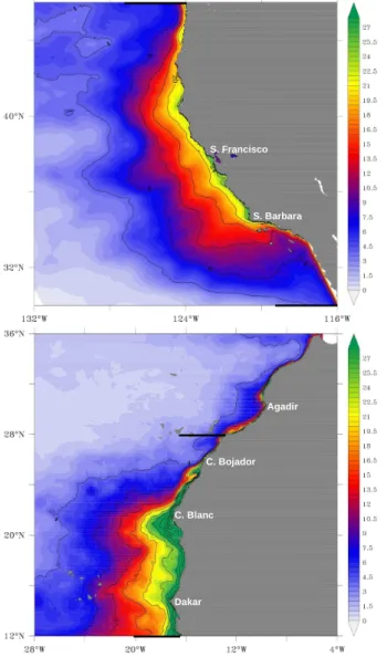
We quantitatively compare the simulations from the two systems as follows: data are averaged for both systems, ex-tending from the coastline to 300 km offshore and over 1◦ bins in meridional direction from 30◦_{N to 46}◦_{N for the} Cal-ifornia CS, and from 12◦_{N to 28}◦_{N for the Canary CS. These} boundaries were chosen to include the most productive re-gions of these upwelling systems (Fig. 4). Thus, the less productive northern parts of the Canary CS are not included in our analyses here.

2.3 Model evaluation

Except for two ecological parameters (the light response pa-rameterαP and phytoplankton mortalityηmort) our

on a newer numerical core optimized for computations on distributed systems (A. Shchepetkin, personal communica-tion, 2008). Additional modifications include an improved implementation of the KPP scheme, a stiffer scheme for the vertical sigma coordinate system and improved numerics for tracer transport. These changes and the new setup for the Ca-nary CS require a re-evaluation of the model’s performance on the basis of primarily satellite chlorophyll and sea-surface temperature (SST), augmented with a monthly climatology of mixed layer depth based on the Argo float observations. We also evaluate the model’s performance with regard to dif-ferent estimates of NPP.

Simulated annual mean surface chlorophyll-a concentra-tions compare generally well to SeaWiFS in both the Cali-fornia CS and the Canary CS, although there is an important underestimation of nearshore concentrations (Fig. 1). The model-data discrepancies in the coastal zone may partially be due to a systematic bias in the SeaWiFS data towards higher concentrations in the coastal waters. Indeed, ocean color remote sensing tends to overestimate chlorophyll gen-erally in continental shelf and coastal regions because of in-creased concentrations of colored optical constituents in the water that vary independently of phytoplankton chlorophyll pigment and absorbing aerosols that tend to be concentrated near the coast (Schollaert et al., 2003; Hyde et al., 2007). This is also consistent with previous results from Gruber et al. (2006) who found similar discrepancies by comparing SeaWiFS chlorophyll with those measured in situ by the Cal-COFI program in this region.

The simulated annual mean SST represents well the ob-served pattern in both the California CS and Canary CS (Fig. 2). In particular, the model successfully captures the offshore extent of the cold upwelling region in both systems. However, as found by Gruber et al. (2006), absolute values of modeled SST exhibit a cold bias of about 1◦C relative to AVHRR satellite data in most of the California CS as well as in the northern Canary CS. Some of the differences be-tween the model and the data likely reflect true changes over time, since our model was forced with heat fluxes from the COADS climatology, which was derived from observations collected between 1950 to 1989, whereas the AVHRR cli-matology was put together on the basis of the years 1997– 2005 only. Therefore, the long-term surface ocean warming observed over the last couple of decades will likely lead to higher SST in AVHRR data in comparison with COADS. In the nearshore areas, overestimated wind stress and uncertain-ties associated with the wind stress profile in the QuikSCAT data is probably further enhancing the cold bias (Capet et al., 2004).

A more quantitative evaluation of the model simulations is depicted in the Taylor (2001) diagrams shown in Fig. 3. A Taylor diagram is anr−θ polar plot that provides a quick quantitative synthesis of three statistics. First, the modeled field’s standard deviation relative to the standard deviation of the observations is represented by the radiusr(distance on

the plot between the model and the origin point). Second, the angle θ between the model point and the X-axis indi-cates the correlation coefficient between the model and the observations. Finally, the distance from the reference point to a given modeled field represents that field’s central pattern root mean square (RMS), also known as the pattern error. If a model were perfect, it would lie along the X-axis, right on top of the (observation) reference point.

For both the California CS and the Canary CS, we find relatively high correlations between simulated and satellite-based annual mean surface chlorophyll ranging between 0.68 for the nearshore area of the California CS up to around 0.9 for the Canary CS when estimated over the entire domain (Fig. 3a). The standard deviations of simulated chlorophyll patterns are, however, 30 % to 50 % lower than in SeaWiFS. This is essentially due to the model underestimating SeaW-iFS’s high values in the immediate nearshore as we men-tioned before. The simulated surface temperatures show high agreement with SST observations from AVHRR (Fig. 3a). In particular, the correlations between modeled and observed patterns are particularly high ranging between 0.95 and 0.99. Finally, the correlation between the simulated mixed layer depth and the Argo-based climatology of de Boyer Mont´egut et al. (2004) is around 0.7 in the California CS and 0.85 in the Canary CS (Fig. 3a). As nearshore MLD observations are associated with relatively large uncertainties (few Argo floats in the coastal areas), only the patterns related to the en-tire domain are represented in the Taylor diagrams. In both systems, the modeled mixed layer depths have substantially larger standard deviations relative to observations. This is likely due to the much coarser resolution of the data (2◦_{) in} comparison to our model’s fine resolution of∼5 km.

The model simulates the seasonal cycle of chlorophyll less successfully than the annual mean pattern (Fig. 3b). In both the California CS and the Canary CS, the correlations of the seasonal anomalies, i.e. of the monthly means minus the an-nual means, range between 0.3 and 0.45. This distinct differ-ence between the annual mean and the seasonal component is not reflected in the SST, which shows generally a very good agreement with observations with a correlation around 0.95 and a model variance very close to the observed one. For the mixed layer depth, the correlations of the seasonal anomalies with observations are 0.75 and 0.82 for the Canary CS and the California CS, respectively. In both systems, the model variance is substantially larger than in observations. Again, this is likely due to the coarse resolution of the mixed layer climatology.

C

a

li

fo

rn

ia

C

S

C

a

li

fo

rn

ia

C

S

C

a

n

a

ry

C

S

Cape Blanc Cape Blanc S. Francisco

S. Francisco

S

e

a

W

iF

S

R

O

M

S

C

a

n

a

ry

C

S

0 0.2 0.4 0.6 0.8 1 1.2 1.4 1.6 1.8 2 4 (mg/m^3)

0 0.2 0.4 0.6 0.8 1 1.2 1.4 1.6 1.8 2 4 0

0.2 0.4 0.6 0.8 1 1.2 1.4 1.6 1.8 2 4

0 0.2 0.4 0.6 0.8 1 1.2 1.4 1.6 1.8 2 4

Fig. 1.Annual average of surface chlorophyll-aconcentrations (mg m−3) from SeaWiFS (top) and ROMS model (bottom) in the California CS (left) and the Canary CS (right). The SeaWiFS climatology is computed over the period from 1997 to 2007.

C

a

li

fo

rn

ia

C

S

C

a

li

fo

rn

ia

C

S

C

a

n

a

ry

C

S

Cape Blanc Cape Blanc S. Francisco

S. Francisco

A

V

H

R

R

R

O

M

S

C

a

n

a

ry

C

S

17 18 19 20 21 22 (°C)

23 24

17 18 19 20 21 22 23 24 11

12 13 14 15 16 17 18 19

11 12 13 14 15 16 17 18 19

Chl-a Chl-a

SST SST

MLD MLD

CanCS CalCS

Chl-a Chl-a

SST SST

MLD MLD

CanCS CalCS Seasonal Anomalies

Fig. 3. Taylor (2001) diagrams of modeled annual-mean (left) and seasonal anomalies (right) of surface chlorophyll (circles), sea surface temperature (diamonds) and mixed layer depth (stars) in the California CS (blue) and the Canary CS (orange). The reference point of the Taylor diagram corresponds to SeaWiFS observations for chlorophyll, AVHRR data for temperature and the monthly climatology of de Boyer Mont´egut et al. (2004) for the mixed layer depth. The statistics were computed separately for the entire domain (data points labeled “1”) and the 100 km wide nearshore region (data points labeled “2”).

underestimates in-situ observation based estimates by over 20 % (Tilstone et al., 2009).

Some of these deficiencies may arise from our using a simple NPZD-type ecosystem model as suggested by Gru-ber et al. (2006) for the underestimation of chlorophyll and NPP in the offshore regions. While the addition of increased biogeochemical and ecological complexity may indeed help, experience shows little gain in model skill for bulk ecosys-tem properties such as chlorophyll and primary production (Friedrichs and Hofmann, 2001; Hood et al., 2003; Friedrichs et al., 2007). Additionally, it has been established that when their parameters are tuned for one type of ecosystems (e.g., EBUS in this study), the simplest NPZD models fit the data as well as those with multiple phytoplankton functional groups (Friedrichs et al., 2007). Moreover, biogeochemical model intercomparisons have revealed that biogeochemical variations tends to be dominated by the physical environment and depend less on ecosystem model complexity (Friedrichs et al., 2006).

Overall, the model exhibits reasonable skills in both up-welling systems. Most importantly, it captures well the strong differences in phytoplankton biomass and NPP that characterizes the California and Canary CS. Since the pri-mary focus of our study here is to understand these differ-ences, we consider the identified biases as acceptable, par-ticularly since the biases in the two systems are of the same nature and go in the same direction.

3 Results and discussion

The Canary CS generally shows substantially higher annual NPP in comparison to the California CS, with the former

hav-Table 1. Comparison of simulated and satellite observation-based estimates of net primary production (mol C m−2yr−1) from Kahru et al. (2009) in the central California CS (34◦N–42◦N).

Offshore extent Kahru ROMS satellite-based model simulated

0–100 km 32.9 21.6 100–500 km 10.9 9.4 500–1000 km 4.7 1.8

Table 2. Comparison of simulated and in-situ estimates of net primary production (mol C m−2yr−1) from Tilstone et al. (2009) over the Canary Current Coastal upwelling (CNRY) biogeochemi-cal province (15◦N–26◦N, 20◦W-African coast) as defined in Til-stone et al. (2009). Simulated NPP is shown at the (N=6) obser-vation point locations and over the whole CNRY biogeochemical province, respectively.

Tilstone ROMS ROMS

in-situ obs model simulated model simulated Tilstone et al. (2009) at obs locations CNRY province

17.3 13.6 19.7

S. Francisco

S. Barbara

C. Blanc C. Bojador

Agadir

Dakar

Fig. 4. Simulated annual mean, vertically integrated NPP (mol C m−2yr−1) in the California CS (left) and Canary CS (right).

40 molCm−2yr−1 in the nearshore areas of the Canary CS south of Cape Bojador. Although these rates are, on aver-age, about 20 % to 40 % lower than corresponding in situ or satellite-based estimates, the model correctly simulates the large difference in NPP between the California CS and the Canary CS. Thus we will be using our model to investigate the mechanisms behind this difference.

According to Eq. (1), NPP is the product of the nutrient limitation termγ (Nn,Nr), the nutrient-unlimited growth rate

µmax_P (T ,I )and the biomassP. Therefore, we need to exam-ine each of these three components in order to understand the contrasting NPP between the two systems.

3.1 Biological production and nutrient resources

As the high biological production in EBUS is driven to the first order by the upwelling of nutrient-rich water to the

sur-0 0.5 1 1.5 2 2.5 3 3.5 4

0 5 10 15 20 25 30 35

f(x) = 1.17x + 8.72 R² = 0.06 f(x) = 4.81x + 7.71

R² = 0.67

Total Inorganic Nitrogen inventory (mol C/m^2)

N

e

t

P

ri

m

a

ry

P

ro

d

u

c

ti

o

n

(

m

o

l

C

/m

^2

/y

r) Canary CS

California CS

(a)

0.2 0.3 0.4 0.5 0.6 0.7 0.8 0.9

0 5 10 15 20 25 30 35

f(x) = 19.88x - 1.9 R² = 0.75 f(x) = 49.72x - 9.34

R² = 0.93

γN

N

e

t

P

ri

m

a

ry

P

ro

d

u

c

ti

o

n

(

m

o

l

C

/m

^

2

/y

r)

Canary CS

California CS

(b)

Fig. 5. (a)The relationship between NPP and the inventory of TIN in the euphotic zone in the California CS (blue) and Canary CS (orange). (b) NPP as a function of the nutrient limitation factor γ (Nn,Nr)averaged over the upper 40 m in the California CS (blue)

and Canary CS (orange). Data were averaged over the 300 km wide nearshore area and over 1◦bins in meridional direction. Circles with horizontal lines correspond to the southernmost part of each system, i.e., from 30◦N to 34◦N for the California CS and from 12◦N to 16◦N for the Canary CS, and circles with vertical lines indicate their northernmost parts, i.e., from 42◦N to 46◦N for the California CS and from 24◦N to 28◦N for the Canary CS.

face, these differences may simply result from contrasting upwelling intensities between the two systems leading to dif-ferent nutrient concentrations in the euphotic zone. To test this hypothesis, we examine here the relationship between NPP and the nutrient content in the euphotic zone in the two upwelling systems (Fig. 5a). To this end, we computed for each system the total inorganic nitrogen TIN (i.e., nitrate and ammonium) integrated vertically over the euphotic zone.

Table 3.Production and its drivers averaged over the 300 km wide nearshore area for the California CS and the Canary CS.Tresidrefers to the

water residence time in the 100 km wide nearshore area.µP andµmax_P refer to the growth rate and nutrient-replete growth rate, respectively.

Nutrient-replete growth ratesµmax_P are normlized to constant PAR=20 W m−2,θ=25 mg C (mg chl-a)−1andT=14◦C, respectively.

NPP TIN T_resid µ_P µmax_P µmax_P µmax_P µmax_P

(I=const) (θ=const) (T =const) Unit mol C m−2yr−1 mol C m−2 day day−1 day−1 day−1 day−1 day−1

California CS 11.8 2.63 19.29 0.32 0.46 0.45 0.52 0.46 Canary CS 18.15 2.17 30.1 0.36 0.64 0.42 0.83 0.57 Relative diff. +54 % −18 % +56 % +12 % +40 % −7 % +60 % +24 %

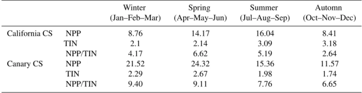
Table 4. Seasonally averaged NPP (mol C m−2yr−1), TIN (mol C m−2) and nutrient assimilation rate (i.e., NPP/TIN in yr−1) in the euphotic zone in the California CS and Canary CS.

Winter Spring Summer Automn (Jan–Feb–Mar) (Apr–May–Jun) (Jul–Aug–Sep) (Oct–Nov–Dec)

California CS NPP 8.76 14.17 16.04 8.41

TIN 2.1 2.14 3.09 3.18

NPP/TIN 4.17 6.62 5.19 2.64

Canary CS NPP 21.52 24.32 15.36 11.57

TIN 2.29 2.67 1.98 1.74

NPP/TIN 9.40 9.11 7.76 6.65

the nutrients are used much more efficiently in the Canary CS relative to the California CS despite the former having actually a higher upwelling intensity, on average (Lachkar and Gruber, 2011; Gruber et al., 2011). Thus, our model re-sults indicate that the reality is more complex than the simple canonical view of higher upwelling giving rise to higher nu-trient availability, yielding higher growth rates and ultimately higher NPP. This perplexing finding emerges not only from the analysis of the annual mean, but also when the analysis is repeated with monthly outputs (Table 4).

In both systems and particularly in the California CS, the relationship between the NPP and TIN exhibits a strong non-linearity, with a tendency for saturation of NPP at high nu-trient concentrations (Fig. 5a). A part of this non-linearity is due to the Michaelis-Menten nutrient limitation formulation, which is strongly non-linear with respect to nutrient concen-trations. Thus, to better describe the relationship between NPP and the “useful” nutrient resources, we show in Fig. 5b NPP as a function of the nutrient limitation factorγ (Nn,Nr).

The slopes of a linear regression of NPP on the nutrient lim-itation factorγ (Nn,Nr)are 20(±7) mol C m−2yr−1for the

California CS and 50 (±8) molCm−2yr−1 for the Canary CS. The more than a factor of two difference in these slopes which represent the productµmax_P (T ,I )×P indicates that these two parameters, i.e., the nutrient-replete growth rate

µmax_P (T ,I )and the biomassP are important drivers for ex-plaining the differing levels of NPP between the Canary and

California CS. Next, we first investigate the contribution of the phytoplankton growth under nutrient-replete conditions and then the contribution of the biomass.

3.2 The nutrient-replete growth rate

The comparison of the two systems reveals that the nutrient-replete growth rateµmax_P (T ,I )is, on average, 40 % faster in the Canary CS than in the California CS (Table 3 & Fig. 6). As described by Eq. (3), µmax_P (T ,I )is a function of light, temperature and the dynamic chlorophyll-to-carbon ratioθ. In order to better understand the contribution of each of these three factors to the overall difference inµmax_P (T ,I )between the two systems, we consider normalizedµmax_P (T ,I ) distri-butions with respect to light, the chlorophyll-to-carbon ratio, and temperature, respectively (Fig. 6).

When normalized to a constant PAR of 20 Wm−2_{, which}

30.5N 32.5N 34.5N 36.5N 38.5N 40.5N 42.5N 44.5N

0 0.1 0.2 0.3 0.4 0.5 0.6 0.7 0.8 0.9 1

Latitude

N

u

tr

ie

n

t-u

n

li

m

it

e

d

g

ro

w

th

(

p

e

r

d

a

y)

California CS

(a)

12.5N 14.5N 16.5N 18.5N 20.5N 22.5N 24.5N 26.5N

0 0.1 0.2 0.3 0.4 0.5 0.6 0.7 0.8 0.9 1

Latitude

N

u

tr

ie

n

t-u

n

li

m

it

e

d

g

ro

w

th

(

p

e

r

d

a

y)

Canary CS

(b)

Fig. 6.Meridional distribution of the temperature-dependent, light-limited growth rate under nutrient replete conditionsµmax_P (T ,I ) in the California CS(a)and the Canary CS(b). Data is horizon-tally averaged over the 300 km wide nearshore area and vertically over the upper 40 m. Shown are the simulatedµmax_P (T ,I )(solid) and normalizedµmax_P (T ,I )to to constant PAR=20 W m−2(long dashed), temperatureT=14◦C (fine dashed) and chlorophyll-to-carbon ratioθ=25 mg C(mg Chl-a)−1(dotted).

by the chlorophyll-to-carbon ratio variations allowed in our model, which mimic photoacclimation in phytoplankton (Falkowski and Raven, 1997). Fixingθ for example at 25 mgC(mgChl−a)−1, which corresponds to the average con-ditions in the central California CS, enhances indeed the difference inµmax_P (T ,I )between the two systems by more than 50 % (Table 3). Finally, when normalized to a con-stant temperature of 14◦_{C (corresponding to the average} tem-perature conditions in the central California CS), the differ-ence inµmax_P (T ,I )between the two systems gets reduced by 38 %, which indicates a smaller, yet important role played by the temperature differences in the contrasting nutrient-replete growth rates between the two upwelling systems (Table 3).

The 40 % largerµmax_P in the Canary CS causes the overall growth rateµP to be 12 % larger in this system, despite a

0.1 0.15 0.2 0.25 0.3 0.35 0.4 0.45 0.5 0.55 0

10 20 30 40 50 60 70 80 90 100

f(x) = 99.98x + 0.25 R² = 0.97 f(x) = 168.08x - 11.4

R² = 0.93

Phytoplankton growth rate (per day)

N

e

t

P

ri

m

a

ry

P

ro

d

u

c

ti

o

n

(

m

m

o

l

C

/

m

^

2

/

d

a

y

)

California CS Canary CS

Fig. 7. The relationship between NPP and the phytoplankton growth rate in the California CS (blue) and Canary CS (orange). Data were averaged over the 300 km wide nearshore area and over 1◦bins in meridional direction. Circles with horizontal lines corre-spond to the southernmost part of each system, i.e., from 30◦N to 34◦N for the California CS and from 12◦N to 16◦N for the Canary CS, and circles with vertical lines indicate their northernmost parts, i.e., from 42◦N to 46◦N for the California CS and from 24◦N to 28◦N for the Canary CS.

stronger nutrient limitation (Table 3). Does this difference alone explain the more than 50 % larger NPP in the Canary CS relative to the California CS? To answer this question, we next consider the effect of the third component in Eq. (1), i.e., the phytoplankton biomass, on the production in the two upwelling systems.

3.3 NPP and phytoplankton biomass

The correlation between the NPP and the total growth rate is very strong in both systems withR2of 0.93 and 0.97 in the Canary and the California systems, respectively. Yet, comparable growth rates in the Canary CS and the Cali-fornia CS lead to substantially different NPP (Fig. 7). The slopes of a linear regression of NPP on the growth rate vary from 100 (±10) molCm−2_{for the California CS to up to 168}

(±28) molCm−2_{for the Canary CS. Since the slope is equal}

to the average biomassP, this difference indicates a signifi-cantly larger average biomass in the Canary CS relative to the California CS even at comparable growth rates. Therefore, in addition to the slightly faster phytoplankton growth in the Canary CS relative to the California CS, mechanisms affect-ing the biomass but independent of the growth rate must con-tribute to the large NPP contrasts between the two systems.

According to Eq. (1), we can write the time-evolution of the phytoplankton biomass as:

dP

dt = [µP(T ,I,Nn,Nr)−8

30.5N 32.5N 34.5N 36.5N 38.5N 40.5N 42.5N 44.5N -0.3 -0.2 -0.1 0 0.1 0.2 0.3 0.4 0.5 0.6 Latitude P h y to p la n k to n b io m a s s s o u rc e s a n d s in k s ( p e r d a y )

California CS

(a)

12.5N 14.5N 16.5N 18.5N 20.5N 22.5N 24.5N 26.5N -0.3 -0.2 -0.1 0 0.1 0.2 0.3 0.4 0.5 0.6 Latitude P h y to p la n k to n b io m a s s s o u rc e s a n d s in k s ( p e r d a y )

Canary CS

(b)

Fig. 8.Meridional distribution of the net growth of phytoplankton (black) and its four components: the growth (green), the grazing (blue), the mortality (red) and the coagulation (yellow) daily rates in the California CS(a)and the Canary CS(b). Data is horizontally averaged over the 300 km wide nearshore area and vertically over the upper 40 m.

−8mort−8coag(P ,DS)] ·P+3(P )

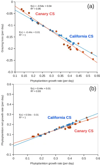
where the term between square brackets on the right-hand side represents the net growth, i.e., growth minus the bio-logical sink terms, and3(P )is the physical transport op-erator. Because of their very small magnitude, the phyto-plankton mortality and the coagulation terms contribute very little to the net growth. Thus, the net growth is essentially set by the balance between phytoplankton growth and the graz-ing by zooplankton (Fig. 8). Moreover, because the grazgraz-ing term8graz(P ,Z)is tightly correlated in our model with the growth rateµP(T ,I,Nn,Nr)(R2>0.95) (Fig. 9a), we can

express the net growth as being nearly proportional to the phytoplankton growth (Fig 9b).

Therefore, if we consider an individual water particle and follow it through time in a Lagrangian framework, Eq. (6)

0.1 0.15 0.2 0.25 0.3 0.35 0.4 0.45 0.5 0.55 -0.3

-0.25 -0.2

-0.15 -0.1 -0.05

0

f(x) = -0.44x + 0.01 R² = 1

f(x) = -0.54x + 0.04 R² = 0.95

Phytoplankton growth rate (per day)

G ra z in g l o s s ( p e r d a y ) Canary CS California CS

(a)

0 0.1 0.2 0.3 0.4 0.5 0.6

-0.1 0 0.1 0.2 0.3 0.4 0.5 0.6

f(x) = 0.54x - 0.01 R² = 1

f(x) = 0.44x + 0.01 R² = 0.93

Phytoplankton growth rate (per day)

P h y to p la n k to n n e t g ro w th ra te (p e r d a y )

California CS

Canary CS

(b)

Fig. 9. (a)The grazing rate as a function of the growth rate in the California CS (blue) and Canary CS (orange). (b)The net growth rate as a function of the growth rate in the California CS (blue) and Canary CS (orange). Data were averaged over the 300 km wide nearshore area and over 1◦bins in meridional direction. Circles with horizontal lines correspond to the southernmost part of each system, i.e., from 30◦N to 34◦N for the California CS and from 12◦N to 16◦N for the Canary CS, and circles with vertical lines indicate their northernmost parts, i.e., from 42◦N to 46◦N for the California CS and from 24◦N to 28◦N for the Canary CS.

can be simplified to:

dP

dt ≈α·µP(T ,I,Nn,Nr)·P , (7)

and the residence timetres of the water parcel in the coastal

zone.

Therefore, it appears that the previously shown partial de-coupling between the growth rate on the one hand and the phytoplankton biomass and NPP on the other hand can result from contrasting residence times in the nearshore area be-tween the two upwelling systems. NPP may indeed remain low despite high growth rates, as the short residence times would prevent the buildup of high phytoplankton biomass. Conversely, long water residence times in the nearshore area can result in a relatively large buildup of biomass, thereby permitting high NPP even at moderate growth rates.

Next, we investigate how water residence times in the nearshore vary between and within these systems, and we explore the potential mechanisms responsible for these vari-ations as well as the impact this has on the recycling and export of nutrients and organic matter.

3.4 Nearshore water residence times

The buildup of biomass in the upwelling zone is a function of the water renewal rate, i.e. the inverse of the residence time, in the nearshore area. To determine the water mass res-idence times in the upwelling zone, a large number of virtual particles were launched in this region and their Lagrangian trajectories computed using ARIANE (Blanke and Raynaud, 1997), a Lagrangian diagnostic tool fully documented at http://stockage.univ-brest.fr/∼_{grima/Ariane/doc.html. In} or-der to obtain a good sampling of newly upwelled waters, we seeded each grid point in the near-surface (upper 10m) and within the 50 km wide coastal strip. Repeating this parti-cle release experiment each 5 days throughout the year led to more than 300 000 particle trajectories in each of the two upwelling systems. Based on these large populations of in-dividual trajectories, we statistically estimated the residence times of newly upwelled water masses in the 100 km wide nearshore area. Because long residence times outside the growing season have little impact on biomass and NPP, we computed for each upwelling system the NPP weighted an-nual mean residence time. This gives a (weighted) average residence time of the newly upwelled water of 30 (±15) days in the nearshore area of the Canary CS, which is more than 55 % longer compared to the residence time found in the Cal-ifornia CS of 19 (±7) days (Fig. 10 and Table 3). Even in the unweighted average case, the difference remains substantial (about 20 %).

The longer water residence times enhance the buildup of biomass in the Canary CS coastal zone, leading to a sub-stantially larger production in comparison with the Califor-nia CS. Conversely, the substantially shorter water residence times in the nearshore region of the California CS result in an overall lower average biomass, thereby contributing to lower-ing the production in this system. Next, we explore the mech-anisms potentially responsible for the identified contrasts in water residence times between the two systems.

30.5 N

32.5 N

34.5 N

36.5 N

38.5

N 40.5

N 42.5

N 44.5

N

0 10 20 30 40 50 60 70 80

Latitude

W

a

te

r

re

si

d

e

n

ce

t

im

e

s

(d

a

y)

California CS

5km

(non-eddy)

5km

(control)

(a)

12.5 N

14.5 N

16.5 N

18.5 N

20.5 N

22.5 N

24.5 N

26.5 N

0 10 20 30 40 50 60 70 80

Latitude

W

a

te

r

re

s

id

e

n

ce

t

im

e

s

(

d

a

y)

5km

(control)

15km

(control)

15km

(narrow shelf)

Canary CS

(b)

Fig. 10. (a)Meridional distribution of the water residence times in the 100 km wide nearshore area in the California CS as simulated in the control simulation (solid black) and the non-eddy simulation (dashed green). (b)Meridional distribution of the water residence times in the 100 km wide nearshore area in the Canary CS as ulated in the control 5 km simulation (solid black), the 15 km sim-ulation with unaltered topography (dashed orange) and the 15 km narrowed-shelf simulation (dashed blue).

3.5 The role of mesoscale activity and shelf topography

0

100

200

300 400 500 600

0

500

1000

1500

2000

2500

3000

3500

4000

4500 Distance to the coast (km)

D

e

p

th

(

m

)

Fig. 11. Alongshore averaged bottom topography depth as a func-tion of distance to the coast in the the Canary CS 15 km simulafunc-tion with unaltered topography (orange) and the 15 km narrowed-shelf simulation (blue).

times in the nearshore area are on average twice as long in the non-eddying simulation in comparison to the control (eddying) simulation. This confirms the important role erted by mesoscale activity in enhancing the offshore ex-port and limiting the local buildup of biomass, in-line with the findings of Gruber et al. (2011) who demonstrated that mesoscale processes increase the transport of nutrient and organic carbon from the nearshore into the open ocean. Sec-ond, to test the role of wide continental shelves in increas-ing water residence times, we made two additional Canary CS simulations at slightly coarser horizontal resolution of 15 km: (i) one simulation where all the settings are kept iden-tical to the control 5 km simulation, and (ii) a second sim-ulation where the initially wide continental shelf was sub-stantially narrowed by altering the nearshore bottom topog-raphy (Fig. 11). The 15 km Canary CS simulation with unal-tered topography shows on average a 12 % longer residence times in comparison to the 5 km simulation (Fig. 10b). This is consistent with our previous finding that lower eddy ac-tivity leads to longer residence times in the nearshore area of EBUS. In the narrowed continental shelf simulation, the water residence times get, however, substantially reduced by 35 % on average (Fig. 10b). This confirms the role of wide continental shelves in enhancing the local recycling and lim-iting the offshore export of nutrients and biomass. Our re-sult is consistent with previous theoretical and model-based findings by Austin and Lentz (2002) and Marchesiello and Estrade (2009). Next, we investigate the consequences of these differences for the recycling and export of nutrients and organic matter in the two upwelling systems.

0 2 4 6 8 10 12 14 16

0 5 10 15 20 25 30

New Production (mol C/ m^2/ yr)

R

e

g

e

n

e

ra

te

d

P

ro

d

u

c

ti

o

n

(

m

o

l

C

/m

^

2

/y

r)

Fig. 12. The relationship between the regenerated production and the new production in the California CS (blue) and Canary CS (or-ange). Data were averaged over the 100 km wide nearshore area and over 1◦bins in meridional direction. Circles with horizontal lines correspond to the southernmost part of each system, i.e., from 30◦N to 34◦N for the California CS and from 12◦N to 16◦N for the Canary CS, and circles with vertical lines indicate their north-ernmost parts, i.e., from 42◦N to 46◦N for the California CS and from 24◦N to 28◦N for the Canary CS.

3.6 Recycling and export of nutrients and organic matter

The inefficient use of nutrients combined with a relatively high offshore export of biomass leads in the California CS relative to the Canary CS to a much lower recycling of nutri-ents in the nearshore area, and thus to a much higher f-ratio, i.e., the ratio of new production to net primary production. Fig. 12 shows the regenerated production as a function of the new production averaged over the first 100 km from the coast in both systems. While new production is only 15 % lower in the California CS in comparison with the Canary CS, regen-erated production is nearly 50 % lower, leading to a substan-tially larger f-ratio in the California CS (0.44) relative to the Canary CS (0.33).

0 2 4 6 8 10 12 14 0

2 4 6 8 10 12 14

f(x) = 0.53x + 1.34 R² = 0.65

f(x) = 1.04x + 0.78 R² = 0.71

New Production (mol C/ m^2/ yr)

E

x

p

o

rt

P

ro

d

u

c

ti

o

n

(

m

o

l

C

/m

^

2

/y

r)

(a)

0 1 2 3 4 5 6 7

0 1 2 3 4 5 6 7

f(x) = 1.32x + 0.06 R² = 0.91 f(x) = 1.33x + 0.43

R² = 0.9

NewProduction (molC/m^yr)

&

x

'

o

rt

P

ro

d

u

c

ti

o

n

(

m

o

l

C

/m

^

2

#

%

)

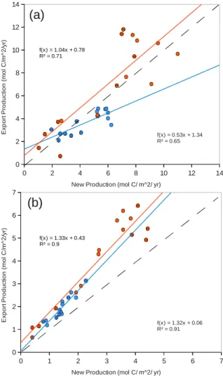
Fig. 13. Export production as a function of new production in the California CS (blue) and Canary CS (orange) averaged(a)over the 300 km wide nearshore area and(b)between 300 km and 500 km offshore. Data were averaged over 1◦bins in meridional direction. Circles with horizontal lines correspond to the southernmost part of each system, i.e., from 30◦N to 34◦N for the California CS and from 12◦N to 16◦N for the Canary CS, and circles with vertical lines indicate their northernmost parts, i.e., from 42◦N to 46◦N for the California CS and from 24◦N to 28◦N for the Canary CS. The diagonal dashed grey line indicate the identity line.

In the California CS, total export production is generally smaller than new production over the first 300 km from the coast, and larger further offshore with regression slopes of 0.53 (±0.22) and 1.32 (±0.23), respectively (Fig. 13). This is consistent with the results of Plattner et al. (2005) who found a substantial spatial decoupling between new and export pro-duction in the California CS with a decoupling length-scale of 300 km. In contrast, in the Canary CS the values of the export and new production are, on average, very simi-lar over the first 300 km from the coast (regression slope of 1.04 (±0.38)), whereas in the 300 km–500 km offshore area the relationship between the new production and the export

production deviate from a 1:1 relationship as is the case in the California CS with nearly identical regression slopes (re-gression slope of 1.33 (±0.25)). We interpret the relatively small differences between export and new production in the nearshore areas of the Canary CS as an indicator of a much weaker decoupling between new and export production in this system in comparison to the California CS.

3.7 Comparison with previous work

Obviously, none of these mechanisms is exclusive of an-other. Yet, the fact that we successfully reproduced the con-trasts in NPP between the Canary and California CS using a simple NPZD-type ecosystem model indicates that phys-ical processes likely dominate in explaining the differences in NPP and biomass between these systems. This needs, however, to be confirmed through a series of simulations per-formed with models that contain more details in terms of bio-geochemical controls (e.g. iron) and/or resolve the ecosys-tem with more phytoplankton functional groups.

4 Summary and conclusions

We investigated the major drivers of the biological produc-tion in EBUS using a comparative modeling study of two of the four major EBUS, namely the California CS and the Canary CS. Our aim has been to identify and compare the production limitations in these two systems, and to explore the mechanisms that control the sensitivity of biological pro-duction to upwelling-favorable wind forcing.

Directly comparable eddy-resolving simulations of the California CS and the Canary CS show that despite nutrient concentrations on average being about 20 % larger in the first, NPP is 50 % larger in the second, indicating a considerably larger nutrient use efficiency in the Canary CS. By analyz-ing phytoplankton growth in nutrient-replete conditions, we found that this more efficient use of nutrients in the Canary CS is essentially due to more favorable light and temperature conditions, resulting in an overall 12 % higher growth rate in the Canary CS in comparison with the California CS. Yet, comparable growth rates in the Canary CS and the California CS are associated with substantially larger productivities in the former. This is due to large contrasts in the water resi-dence times in the nearshore between the two systems.

We found that the newly upwelled water stays on average more than 50 % longer in the nearshore area of the Canary CS relative to the California CS. This enhances the buildup of biomass in the coastal zone of the Canary CS and leads to higher production, larger local recycling of nutrients, and much weaker decoupling between new and export produc-tion. Additional simulations demonstrate that the wider shelf and the lower level of mesoscale activity in the Canary CS relative to the California CS both likely contribute to the longer water residence time in the former.

Overall, our results show that factors affecting timescales of biological growth such as the light and temperature and those related to the dynamics of the cross-shore circulation in coastal upwelling systems such as the shelf topography and the level of eddy activity exert a strong control on nu-trient use efficiency, and thus, on the sensitivity of biologi-cal production to the intensity of upwelling. Therefore, this study suggests that the biological response to climate change induced perturbations such as upwelling favorable wind in-tensification (e.g. Bakun, 1990) or increased stratification

(e.g. Rykaczewski and Dunne, 2010) might lead to contrast-ing biological responses in the California CS and the Canary CS, with major implications for the biogeochemical cycles and fisheries in these two ecosystems.

Acknowledgements. Support for this research has come from the Swiss Federal Institute of Technology Zurich (ETH Zurich). Computations were performed at the central computing cluster of ETH Zurich, Brutus. We are indebted to J. McWilliams and his research group for the development, maintenance, and sharing of the physical component of ROMS. We thank H. Frenzel and D. Loher for their code support. We are grateful to B. Blanke and N. Grima for making their ARIANE code available. We also thank the various providers of the satellite data, in partic-ular the SeaWiFS Project (Code 970.2) sponsored by NASA’s Mission to Planet Earth program, as well as the AVHRR data products sponsored by the NOAA/NASA Polar Pathfinder program.

Edited by: G. Herndl

References

Allen, J.: Upwelling and Coastal Jets in a Continuously Stratified Ocean, J. Phys. Oceanogr., 3, 245–257, 1973.

Ar´ıstegui, J., Barton, E. D., Tett, P., Montero, M. F., Garca-Muoz, M., Basterretxea, G., Cussatlegras, A., Ojeda, A., and de Armas, D.: Variability in plankton community structure, metabolism, and vertical carbon fluxes along an upwelling fil-ament (Cape Juby, NW Africa), Progr. Oceanogr., 62, 95–113, doi:10.1016/j.pocean.2004.07.004, 2004.

Ar´ıstegui, J., Barton, E. D., Alvarez-Salgado, X. A., Santos, M., Figuerias, F.G., Kifani, S., Hernandez-Leon, S., Mason, E., Machu, E., and Demarcq, H.: Sub-regional ecosystem variability in the Canary Current upwelling, Progr. Oceanogr., 83, 33–48, doi:10.1016/j.pocean.2009.07.031, 2009.

Austin, J. A. and Lentz, S. J.: The Inner Shelf Response to Wind-Driven Upwelling and Downwelling, J. Phys. Oceanogr., 32, 2171–2193, 2002.

Bakun, A.: Global Climate Change and Intensification of Coastal Ocean Upwelling, Science, 247, 198–201, doi:10.1126/science.247.4939.198, 1990.

Barnier, B., Siefried, L., and Marchesiello, P.: Thermal forcing for a global ocean circulation model using a three-year climatology of ECMWF analyses, J. Mar. Syst., 6, 363–380, 1995.

Beckmann, A. and Haidvogel, D. B.: Numerical simulation of flow around a tall isolated seamount. Part I: Problem formulation and model accuracy, J. Phys. Oceanogr., 23, 1736–1753., 1993. Berger, W. H., Smetacek, V. S. and Wefer, G.: Ocean

productiv-ity and paleoproductivproductiv-ity–An overview, in Productivproductiv-ity of the Ocean: Present and Past, edited by: Berger, W. H., Smetacek, V. S., and Wefer, G., 1–35, John Wiley, Hoboken, N. J., 1989. Blanke, B. and Raynaud, S.: Kinematics of the Pacific Equatorial

Undercurrent: an Eulerian and Lagrangian approach from GCM results, J. Phys. Oceanogr., 27, 1038–1053, 1997.

Carr, M.: Estimation of potential productivity in Eastern Boundary Currents using remote sensing, Deep Sea Res. Pt. II, 49, 59–80, doi:10.1016/S0967-0645(01)00094-7, 2001.

Carr, M. and Kearns, E. J.: Production regimes in four Eastern Boundary Current systems, Deep Sea Res. Pt. II, 50, 3199–3221, doi:10.1016/j.dsr2.2003.07.015, 2003.

Capet, X. J., Marchesiello, P., and McWilliams, J. C.: Upwelling re-sponse to coastal wind profiles, Geophys. Res. Lett., 31, L13311, doi:10.1029/2004GL020123, 2004.

Chase, Z., Strutton, P. G., and Hales, B.: Iron links river runoff and shelf width to phytoplankton biomass along the U.S. West Coast, 2007.

Chassignet, E. P. and Verron, J.: Ocean Weather Forecasting: An Integrated View of Oceanography, Springer, Dordrecht, The Netherlands, 2006.

Chavez, F. P. and Toggweiler, J. R.: Physical estimates of global new production: The upwelling contribution, in: Upwelling in the Ocean: Modern Processes and Ancient Records, edited by: Summerhayes, C. P., Emeis, K.-C., Angel, M. V., Smith, R. L., and Zeitzschel, B., 313–320, ISBN:978-0471960416, John Wi-ley, New York, 1995.

Chavez, F. P. and Messi´e, M.: A comparison of Eastern Boundary Upwelling Ecosystems, Prog. Oceanogr., 83, 80–96, doi:10.1016/j.pocean.2009.07.032, 2009.

Chelton, D. B., deSzoeke, R. A., Schlax, M. G., Naggar, K. E., and Siwertz, N.: Geographical variability of the first-baroclinic Rossby radius of deformation, J. Phys. Oceanogr., 28, 433–460, 1998.

da Silva, A. M., Young, C. C., and Levitus, S.: Atlas of surface ma-rine data 1994. Volume 1: algorithms and procedures, Technical Report NOAA Atlas NESDIS 6, National Oceanic and Atmo-spheric Administration, Washington, DC, 1994.

de Boyer Mont´egut, C., Madec, G., Fischer, A. S., Lazar, A., and Iudicone, D.: Mixed layer depth over the global ocean: an exam-ination of profile data and a profile-based climatology, J. Geo-phys. Res., 109, C12003, doi:10.1029/2004JC002378, 2004. Demarcq, H.: Trends in primary production, sea surface

tem-perature and wind in upwelling systems (1998–2007), Prog. Oceanogr., 83, 376–385, doi:10.1016/j.pocean.2009.07.022, 2009.

Falkowski, P. G. and Raven., J.: Aquatic Photosynthesis, Blackwell, Oxford 375 pp, 1997.

FAO: The State of World Fisheries and Aquaculture 2008, Food & Agriculture Org, Pap/Cdr edn., 2009.

Eppley, R. W.: Temperature and phytoplankton growth in the sea, Fish. Bull., 70, 1063–1085, 1972.

Eppley, R. W. and Peterson, B. J.: Particulate organic matter flux and planktonic new production in the deep ocean, Nature, 282, 677–680, 1979.

Friedrichs, M. A. M. and Hofmann, E. E.: Physical control of bio-logical processes in the central equatorial Pacific Ocean, Deep-Sea Res. Pt. I, 48, 1023–1069, 2001.

Friedrichs, M. A. M., Hood, R. H., and Wiggert, J. D.: Ecosys-tem model complexity versus physical forcing: Quantification of their relative impact with assimilated Arabian Sea data, Deep-Sea Res. Pt. II, 53, 576–600, 2006.

Friedrichs, M. A. M., Dusenberry, J. A., Anderson, L. A., Arm-strong, R. A., Chai, F., Christian, J. R., Doney, S. C., Dunne, J., Fujii, M., Hood, R., Mcgillicuddy, D. J., Moore, J. K.,

Schar-tau, M., Spitz, Y. H., and Wiggert, J. D.: Assessment of skill and portability in regional marine biogeochemical models: Role of multiple planktonic groups, J. Geophys. Res.-Oceans, 112, C08001, 22 pp., doi:10.1029/2006JC003852, 2007.

Fung, I., Meyn, S. K., Tegen, I., Doney, S., John, J., and Bishop, J.: Iron supply and demand in the upper ocean, Global Biogeochem. Cy., 14, 281–295, 2000.

Gruber, N., Frenzel, H., Doney, S. C., Marchesiello, P., McWilliams, J. C., Moisan, J. R.., Oram, J., Plattner, G.-K., and Stolzenbach, K. D..: Eddy-resolving simulation of plankton ecosystem dynamics in the California Current System, Deep-Sea Res. Pt. I, 53, 1483–1516, doi:10.1016/j.dsr.2006.06.005. 2006 Gruber, N., Lachkar, Z., Frenzel, H., Marchesiello, P., Munnich, M.,

McWilliams, J. C., Nagai, T., and Plattner, G.: Mesoscale eddy-induced reduction of biological production in coastal upwelling systems, Nat. Geosci., doi:10.1038/ngeo1273, 2011.

Hood, R. R., Kohler, K. E., McCreary, J. P., and Smith, S. L.:A four-dimensional validation of a coupled physical-biological model of the Arabian Sea, Deep-Sea Res. Pt. II, 50, 2917–2945, 2003. Hyde, K., O’Reilly, J., and Oviatt, C.: Validation of SeaWiFS

chlorophyll-ain Massachusetts Bay, Cont. Shelf Res., 27, 1677– 1691, 2007.

Jickells, T. D, An, Z. S., Andersen, K. K., Baker, A. R., Berga-metti, G., Brooks, N., Cao, J. J, Boyd, P. W., Duce, R. A., Hunter, K. A., Kawahata, K., Kubilay, N., laRoche, J., Liss, P. S., Mahowald, N., Prospero, J. M., Ridgwell, A. J., Tegen, I., and Torres., R.: Global Iron Connections Between Desert Dust, Ocean Biogeochemistry, and Climate, Science, 308, 5718, 67– 71, doi:10.1126/science.1105959, 2005.

Kahru, M., Kudela, R., Manzano-Sarabia, M., and Mitchell, B. G.: Trends in primary production in the California Current detected with satellite data, J. Geophys. Res., 114, C02004, doi:10.1029/2008JC004979, 2009.

Lachkar, Z. and Gruber, N.: A comparative study of biological production in eastern boundary upwelling systems using an ar-tificial neural network, Biogeosciences Discuss., 8, 9901–9941, doi:10.5194/bgd-8-9901-2011, 2011.

Large, W. G., McWilliams, J. C., and Doney, S. C.: Oceanic vertical mixing: A review and a model with a nonlocal boundary layer parameterization, Reviews of Geophys. Res., 32, 363–403, 1994. Mackas, D. L., Strub, P. T., Thomas, A., and Montecino, V.: Eastern ocean boundaries, vol. 2 ofThe Sea/, edited by: Robinson, A. R. and Brink, K. H., 21–59, Harvard University Press, 2006. Marchesiello, P., McWilliams, J. C., and Shchepetkin, A. F.:

Open boundary conditions for long-term integration of regional oceanic models, Ocean Modell., 3, 1–20, 2001.

Marchesiello, P., McWilliams, J. C., and Shchepetkin, A. F.: Equi-librium structure and dynamics of the California Current system, J. Phys. Oceanogr., 33, 753–783, 2003.

Marchesiello, P. and Estrade, P.: Eddy activity and mixing in upwelling systems: a comparative study of Northwest Africa and California regions, Int. J. Earth Sci., 98, 299–308, doi:10.1007/s00531-007-0235-6, 2009.

McGregor, H. V., Dima, M., Fischer, H. W., and Mulitza, S.: Rapid 20th-Century Increase in Coastal Upwelling off Northwest Africa, Science, 315, 637–639, doi:10.1126/science.1134839, 2007.

current systems, Prog. Oceanogr., 53, 141–162, ISSN:0079– 6611, doi:10.1016/S0079-6611(02)00028-9, 2002.

Minas, H. J., Minas, M., and Packard, T. T.: Productivity in up-welling systems deduced from hydrographic and chemical fields, Limnol. Oceanogr., 31, 1182–1206, 1986.

Muller-Karger, F. E., Varela, R., Thunell, R., Luerssen, R., Hu, C., and Walsh, J. J.: The importance of continental margins in the global carbon cycle, Geophys. Res. Lett., 32, L01602, doi:10.1029/2008JC004979, 2005.

Pauly, D. and Christensen, V.: Primary production re-quired to sustain global fisheries, Nature, 374, 255–257, doi:10.1038/374255a0, 1995.

Plattner, G. -K., Gruber, N., Frenzel, H., and McWilliams, J. C.: De-coupling marine export production from new production, Geo-phys. Res. Lett., 32, L11612, doi:10.1029/2005GL022660, 2005. Risien, C. M. and Chelton, D. B.: A global climatology of surface wind and wind stress fields from eight years of QuikSCAT scat-terometer data, J. Phys. Oceanogr., 38, 2379–2413, 2008. Rossi, V., C. L´opez, C., Sudre, J., Hern´andez-Garca, E., and

Garc¸on, V.: Comparative study of mixing and biological activity of the Benguela and Canary upwelling systems, Geophys. Res. Lett., 35, L11602, doi:10.1029/2008GL033610, 2008.

Rykaczewski, R. R. and Dunne, J. P.: Enhanced nutrient supply to the California Current Ecosystem with global warming and increased stratification in an earth system model, Geophys. Res. Lett., 37, L21606, doi:10.1029/2010GL045019, 2010.

Schollaert, S. E., Yoder, J. A., O’Reilly, J. E., Westphal, D. L.: Influence of dust and sulfate aerosols on ocean color spec-tra and chlorophyll a concentrations derived from SeaWiFS off the US east coast, J. Geophys. Res., 108, 3191, 1–13, doi:10.1029/2000JC000555, 2003.

Shannon, L., Crawford, R., Pollock, D., Hutchings, L., Boyd, A., Taunton-Clark, J., Badenhorst, A., Melville-Smith, R., Au-gustyn, C., Cochrane, K., Hampton, I., Nelson, G., Japp, D., and Tarr, R.: The 1980s a decade of change in the Benguela ecosystem, South African Journal of Marine Science, 12, 271– 296, 1992.

Shchepetkin, A. F. and McWilliams, J. C.: Quasi-monotone advec-tion schemes based on explicit locally adaptive dissipaadvec-tion, Mon. Weather Rev., 126, 1541–1580, 1998.

Shchepetkin, A. F. and McWilliams, J. C.: The regional oceanic modeling system (ROMS): A split-explicit, free-surface, topography- following-coordinate oceanic model, Ocean Modell. IX, 347–404, Hooke Inst. Oxford Univ., Oxford, U. K., 2005. Smith, W. H. F. and Sandwell, D. T.: Global seafloor topography

from satellite altimetry and ship depth soundings, Science, 277, 1957–1962, 1997.

Taylor, K. E.: Summarizing multiple aspects of model performance in a single diagram, J. Geophys. Res., 106, 7183–7192, 2001. Tilstone, G., Smyth, T., Poulton, A., and Hutson, R.: Measured and

remotely sensed estimates of primary production in the Atlantic Ocean from 1998 to 2005, Deep Sea Res. Pt. II, 56, 918–930, doi:10.1016/j.dsr2.2008.10.034, 2009.

Thomas, A. C., Carr, M.-E., and Strub, P. T.: Chlorophyll variability in Eastern Boundary Currents, Geophys. Res. Lett., 28, 3421– 3424, 2001.