Autonomous electronic water meter based on hydrogeneration

M

l:fJ

Tiago Filipe

Lagarinhos Monte

AUTONOMOUS ELECTRONIC WATER METER

BASED ON HYDROGENERATION

CONTADOR DE ÁGUA ELECTRÓNICO AUTÓNOMO

BASEADO EM HIDROGERAÇÃO

li(!

ttJ

Tiago Filipe

Lagarinhos Monte

AUTONOMOUS ELECTRONIC WATER METER

BASED ON HYDROGENERATION

CONTADOR DE ÁGUA ELECTRÔNICO AUTÔNOMO

BASEADO EM HIDROGERAÇÃO

Dissertação apresentada à Universidade de Aveira para cumprimento dos requisitos necessários à obtenção do grau de Mestre Engenharia Electrónica e Telecomunicações, realizada sob a orientação científíca do Praf. Dr. Rui Manuel Escadas Ramos Martins, Professor Auxiliar do Departamento de Electrónica, Telecomunicações e Informática da Universidade de Aveiro

SDUA

1I,Im,IImn

o júri Presidente

Orientador

Arguente

José Carlos Esteves Duarte Pedro

Professor Catedrático do Departamento de Electrónica, Telecomunicações e Informática da Universidade de Aveiro

Rui Manuel Escadas Ramos Martins

Professor Auxiliar do Departamento de Electrónica, Telecomunicações e Informática da Universidade de Aveiro

José Miguel Costa Dias Pereira

Professor Coordenador do Departamento de Sistemas e Informática da Escola Superior de Tecnologia de Setúbal

agradecimentos Gostaria de expressar a minha gratidão para com o meu orientador, Prof. Rui Manuel Escadas Ramos Martins, pela sua colaboração, ajuda, apoio e disponibilidade no desenrolar deste trabalho de mestrado. Da mesma forma, gostaria de agradecer aos Engenheiros Carlos Alves e Cláudio Monteiro, e à restante equipa da empresas Globaltronic e HFA, pela forma acolhedora como me receberam e por todo o apoio que me prestaram sempre que necessitei do seu auxílio.

Por último quero agradecer à minha família, em especial aos meus pais e à minha namorada, pelo apoio que me têm dado ao longo de todo o meu percurso acadêmico.

palavras-chave Hidrogeração, microcontroladores, ultra condensadores, electrónica de baixa potência, telemetria

resumo Esta tese tem como objectivo relatar o desenvolvimento de um sistema electrónico baseado em energias renováveis, mais especificamente, um contador de água electrónico baseado em hidrogeração.

O trabalho foi iniciado com um estudo das características do

hidrogerador que iria ser utilizado, que foi desenvolvido pela Vulcano (sub-holding da Bosch) e utilizado em esquentadores de aquecimento de água para produzir a faísca de ignição.

De seguida, e após a selecção do método de armazenamento de energia (ultra condensadores), procedeu-se ao desenvolvimento de um sistema para demonstração da simplicidade na determinação do SOC nestes dispositivos. A carga é monitorizada por um microcontrolador e os dados são visualizados num computador pessoal através de um interface gráfico desenvolvido em C#.

Procedeu-se depois ao desenvolvimento do projecto de hardware e software do contador de água electrónico. Ambos foram feitos com o objectivo primário de obter o máximo de eficiência energética,

mantendo uma boa performance geral do sistema. Fez-se ainda uma PCB para o hardware desenvolvido.

keywords Hydrogeneration, microcontrollers, ultra capacitors, low power electronics, telemetry

abstract This thesis aims to report the develolment of an electronic system based on renewable energies, specifically, an electronic water meter based on hydrigeneration.

The thesis work was initiated by studying the hydrogenerator’s

characteristics, which is a device developed by Vulcano (a Bosch sub-holding) and is used in water heaters to generate the ignition spark.

Following, and after selecting which energy storage method would be used, a charge monitoring system was developed. It aims to

demonstrate how simple it can be to determine the SOC of ultracapacitors, when compared with batteries. The charging is monitorized by a microncontroller and the data is displayed on a computer, using a graphical interface developed in C#.

It was then developed the water meter’s hardware and software project. Both had the primary objective of obtaining maximum energy efficiency,

while maintaining a good overall system performance.A PCB was also

Contents

1 INTRODUCTION 7

1.1 Motivation . . . 7

1.2 Objectives . . . 7

1.3 Thesis Structure . . . 8

2 STATE OF THE ART AND GENERAL CONCEPTS 9 2.1 Water Meters . . . 9 2.1.1 Positive Displacement . . . 10 2.1.1.1 Nutating disc . . . 10 2.1.1.2 Oscillating piston . . . 10 2.1.2 Velocity . . . 11 2.1.2.1 Turbine meter . . . 11 2.1.2.2 Venturi meter . . . 12 2.1.2.3 Orifice meter . . . 12 2.1.2.4 Ultrasonic meter . . . 13 2.1.2.5 Magnetic meter . . . 14 2.1.2.6 Electronic meter . . . 15

2.1.3 Remote transmission meters . . . 15

2.2 Electrical Energy Storage Systems . . . 16

2.2.1 Batteries . . . 17

2.2.2 Electric double-layer capacitors . . . 18

2.2.2.1 UC applications . . . 21

2.2.3 Choosing the energy storage system . . . 24

2.2.3.1 Conclusion . . . 25

2.3 Hydro generation . . . 25

2.3.1 History of hydro generation . . . 25

2.3.2 The world’s smallest hydro generator . . . 27

2.3.3 Hydro generator study . . . 28

2.3.3.1 AC characteristics . . . 28

2.3.3.2 Laboratory testing . . . 29

2.3.3.3 Power factor correction and maximum power transfer . . . . 30

3 UC CHARGING AND SOC MONITORING SYSTEM 35 3.1 Introduction . . . 35

3.2 HDG and rectifying bridge . . . 35

3.3 Microcontroller . . . 37

3.4 Graphical user interface . . . 38

4 WATER METER PROJECT - HARDWARE 41 4.1 Introduction . . . 41 4.2 Energy storage . . . 42 4.3 LCD . . . 42 4.4 GSM modem . . . 44 4.5 Microcontroller . . . 48 4.6 PCB . . . 50 4.7 Conclusion . . . 51

5 WATER METER PROJECT - SOFTWARE 52 5.1 Meetering process . . . 52

5.2 Functions overview . . . 53

5.3 System’s general fluxogram . . . 54

5.4 Conclusion . . . 55

6 Conclusions 56 6.1 Final system analysis . . . 56

6.2 Future work . . . 57

List of Figures

2.1 Nutating disc (taken from www.engineersedge.com) . . . 10

2.2 Oscillating piston (taken from www.smartmeasurement.com) . . . 11

2.3 Turbine meter (taken from www.smartmeasurement.com) . . . 12

2.4 Venturi meter (taken from www.smartmeasurement.com) . . . 12

2.5 Orifice meter (taken from www.flowconditioner.com) . . . 13

2.6 Ultrasonic doppler meter (taken from www.omega.com) . . . 14

2.7 Magnetic meter (taken from www.wikipedia.org) . . . 15

2.8 Electrical energy storage methods . . . 16

2.9 Various batteries with different shapes and voltages (taken from www.wikipedia.org) 17 2.10 Capacitor diagram (taken from www.wikipedia.org) . . . 19

2.11 UC diagram (taken from www.wikipedia.org) . . . 20

2.12 The UC bus at a bus stop (taken from www.youtube.com) . . . 22

2.13 Batteries/UC hybrid energy storage system (taken from www.afstrinity.com) . 23 2.14 Honda’s FCX UC bank (taken from www.honda.com) . . . 23

2.15 Energy and Power Density (taken from www.wikipedia.org) . . . 24

2.16 Three Gorges Dam (taken from www.wikipedia.org) . . . 26

2.17 Vulcano hydro generator (taken from www.vulcano.pt) . . . 27

2.18 Frequency and peak-to-peak voltage Vs Water flow . . . 28

2.19 Frequency and peak voltage Vs Water flow (up to 2.5 L/min) . . . 29

2.20 Output voltage with different capacitors . . . 30

2.21 Power transfer . . . 31

2.22 Equivalent circuit with parallel load impedance . . . 31

2.23 Equivalent circuit with series load impedance . . . 32

2.24 Output capacitors . . . 33

2.25 Ultra cap charging . . . 34

3.1 HDG and rectifying diode bridge . . . 36

3.2 HDG output with paralell 1uF capacitor and no load . . . 36

3.3 HDG output with connected circuit . . . 37

3.4 Microcontroller . . . 37

3.5 Software fluxogram . . . 38

3.6 Graphical user interface . . . 39

3.7 Graphical user interface software fluxogram . . . 39

4.1 HDG, diode bridge and UCs schematic . . . 42

4.2 LCD . . . 43

4.3 5V Regulator . . . 43

4.4 LCD schematic . . . 44

4.5 GC864 top view . . . 44

4.7 GSM modem schematic . . . 46

4.8 Modem ON/OFF . . . 47

4.9 Voltage Vs Frequency . . . 48

4.10 Microcontroller and attached electronics schematic . . . 49

4.11 PCB . . . 50

4.12 PBC, antenna and hydrogenerator . . . 51

5.1 HDG’s interrupt process . . . 52

List of Tables

2.1 Battery types and characteristics . . . 18

2.2 Self discharge test . . . 21

2.3 Batteries pros and cons . . . 24

Nomenclature

ADC Analog to Digital Converter

EDLC Electric Double-Layer Capacitors

GSM Global System for Mobile Communications GUI Graphical user interface

HDG Hydro Generator

IDE Integrated Development Environment LCD Liquid Crystal Display

LDO Low-Dropout

MPPT Maximum Power Point Transfer NiCd Nickel-cadmium

NiMh Nickel-metal hydride OC Open Circuit

PLC Power Line Communications QFN Quad Flat No leads

ROC Rate of charge RTC Real Time Clock SC Supercapacitors SOC State of Charge

UC Ultracapacitors

USART Universal Synchronous Asynchronous Receiver Transmitter WF Water Flow

Chapter 1

INTRODUCTION

1.1

Motivation

From my own experience, the monthly water bill is usually an estimative, most of the times above the real value. To avoid overcharging, it is necessary a visual checking of the wa-ter mewa-ter by either the user or an employee from the service provider. There is always the chance that the user doesn’t send the correct data, or simply doesn’t send any data. Therefor, periodical readings must be done by an employee from the service provider, which comes, obviously, with some costs.

This problem could easily be solved using telemetry solutions. Furthermore, this solu-tions could consist of water meters able to transmit data remotely, eliminating the need of human intervention.

There are such water meters, but the drawback is that they depend on an external energy source (usually a battery pack). Batteries have a limited lifetime, so they required periodical replacement.

The motivation for this project is the development of an energetically self-sustained water meter. Such a device would have numerous advantages, namely, low maintenance needs, remote data transmission capabilities and being environmentally friendly.

1.2

Objectives

This thesis aims for the development of an autonomous electronic water meter capable of remote data communication, in order to eliminate human intervention in the reading process. The water meter will be based on a hydrogenerator developed by Vulcano (Bosch Subholder) and plays a double role in the system: energy source and WF measurement instrument. Its output is simultaneously used to measure the water flow (which will be explained further ahead) and to convert some of the water’s kinetic energy in electrical energy.

An analysis of the hydrogenerator is required, to be conscious of its characteristics and capabilites, and taking the most advantage of this device to achieve maximum performance. To make the water meter energetically self-sufficient, the converted energy must be stored either in batteries or other possible technologies, namely, UC technology.

Since it is a purely electronic system, it will have to be controlled by a microcontroller unit. The most recent generations of 8-bit microcontrollers have very low power consumptions, making them perfect for this kind of applications.

For remote data transmission, GSM seems to be the most reliable and universal solu-tion. For this reason, a GSM modem will be included in the system. For local readings (if

necessary), the system will have a simple LCD display triggered by a reading button. The final prototype is intended for the normal household of 3+ persons, being able to record all water consumptions and reporting them to the respective service provider. If intended, the user can make a visual checking of the water usage.

1.3

Thesis Structure

On this chapter the main objectives of this thesis are presented.

Chapter 2 is used to describe the state of the art regarding water meters and electrical storage technologies. It gives a general view on various types of commercially available wa-ter mewa-ters, divides them in categories and explains how the most common types work. Also, it describes the some of the characteristics of batteries and UC , followed by a discussion on which technology should be used for this project. Finally, the analysis of the hydrogenerator is presented, which includes field and laboratory testings and results.

On chapter 3 it is described a charge monitoring system for UC. This was developed with the goal of getting familliared with the UC technology and demonstrating how the SOC determination is done.

Chapter 4 describes the hardware development for the water meter prototype. Explains the main blocks and their functions.

Chapter 5 describes the software implemented, the method used for water metering, some of the more important functions and the general fluxogram of the system.

Chapter 2

STATE OF THE ART AND GENERAL

CONCEPTS

2.1

Water Meters

Water Meters are devices used to measure the volume of water usage. In most developed countries, they are used at each residential and commercial building in a public water supply system. The total usage is usually displayed in cubic feet (f t3_{), cubic meters (m}3_{) or US}

gallons. It can either be a mechanical or electronic register, and some water meters can also display instant water flow along with the total value.

They’re used all over the world, and have become an important utility for some of the following reasons[1]:

• They make it possible to charge costumers in proportion to the amount of water they use;

• They allow the system to demonstrate accountability;

• They are fair for all costumers because they record specific usage;

• They encorage costumers to conserve water (especially as compared to flat rates); • They allow a utility system to monitor the volume of finished water it puts out; • They aid in the detection of leaks and waterline breaks in the distribution system. Water meters are generally owned, read, and maintained by a public water provider such as a city, rural water association, or private water company.

Those used in typical water distribution system as designed for cold potable water only. For other types of water, special meters are used. For instance, hot water meters are de-signed with special materials that can withstand higher temperatures[2].

Meters are classified into two basic types, positive displacement and velocity, but with many variatons of each. There are also meters who combine both methods, called com-pound meters. These use a valve machanism to direct water flow into each part of the meter so readings can be taken from both mechanisms[3]. Follows a resume of some of the most used types of water metering systems.

2.1.1 Positive Displacement

Positive displacement meters are generally very accurate measuring low to moderate flow rates, therefore used in most homes, apartments, hotels and office buildings[3]. They oper-ate by measuring woper-ater flow against a known volume of liquid held in a small chamber. The compartment moves with the flow of water and is repeatedly filled and emptied. The flow rate is then calculated based on the number of times this chamber is filled and emptied.

They usually have a built-in strainer to protect the measuring element from rocks or other debris that could stop or break the measuring element. Normally have bodies made of bronze, brass or plastic, with internal measuring chambers made from molded plastics and stainless steel[2].

The data is recorded using an arrangement of gears driven by a magnet, which is moved by either a nutating disc or an oscillating piston. This magnetic drive principle is used so that liquid doesn’t come in contact with parts.

2.1.1.1 Nutating disc

Nutating disc (or wobble) meters are the most common type of displacement meters. This type of flow meter is normally used for water service, such as raw water supply. The movable element is a circular disc which is attached to a central ball. A shaft is fastened to the ball and held in an inclined position by a cam or roller. The disk is mounted in a chamber which has spherical side walls and conical top and bottom surfaces. The fluid enters an opening in the spherical wall on one side of the partition and leaves through the other side. As the fluid flows through the chamber, the disc wobbles (hence the name wobble) or executes a nutating motion. Since the volume of fluid required to make the disc complete one revolution is known, the total flow through a nutating disc can be calculated by multiplying the number of disc totations by the known volume of fluid.

The rotating motion of the disc operates a revolution counter, through a crank and a set of gears which is calibrated to indicate total system flow [1][4].

Figure 2.1: Nutating disc (taken from www.engineersedge.com)

2.1.1.2 Oscillating piston

Piston meters have a piston that oscillates back and forth as water flows through a precision-machined chamber containing that said piston. The position of the piston divides the cham-ber into compartments containing an exact volume. Liquid pressure drives the piston to oscillate and rotate on its center hub. The movements of the hub are sensed through the meter wall by a follower magnet. Each revolution of the piston hub is equivalent to a fixed volume of fluid, which is transmited to a register through an arrangement of magnetic drive and gear assembly[5].

Figure 2.2: Oscillating piston (taken from www.smartmeasurement.com)

2.1.2 Velocity

Velocity meters operate on the principle that water passing through a know cross-section with a measured velocity can be equated into a volume of flow. They are mostly used for high flows of water, being used typically in large industries with a high water consumption. There are several types of velocity based meters: turbine, venturi, orifice, ultrasonic and magnetic, just do name a few. The ultrasonic and magnetic meters do not have mechanical measuring elements, they need electronic devices to make the measures[1, 2].

The following subsubsections contain a brief explanation of the refered water meter types 2.1.2.1 Turbine meter

Turbine meters have a rotating element that turns with the flow of water. Volume of water is measured by the number of revolutions of the rotor. The rotational speed is a direct function of flow rate and can be sensed by a magnetic pick-up, photoelectric cell, or gears[6]. They are less accurate at low flow rates.

The flow direction is generally straight through the meter, allowing for higher flow rates and less pressure loss than displacement type meters. They’re used for large commercial users, fire protection, and as master meters for the water distribution system. Strainers are usually installed in front of the meter to protect the measuring element from gravel or other debris[1, 2].

Figure 2.3: Turbine meter (taken from www.smartmeasurement.com)

2.1.2.2 Venturi meter

Venturi meters are used to measure the flow through a pipeline. They have a section that has a smaller diameter than the pipe on the upstream side. Based on a principle of hydraulics, as water flows through the pipe, its velocity is increased as it flows through a reduced cross-sectional area. Difference in pressure before water enters the smaller diameter section and at the smaller diameter “throat” is measured. The change in pressure is proportional to the square of velocity. Flow rate can be determined by measuring the difference in pressure. Venturi meters are suitable for large pipelines and do not require much maintenance[1].

Figure 2.4: Venturi meter (taken from www.smartmeasurement.com)

2.1.2.3 Orifice meter

Like venturi meters, orifice meters are used to measure flow rate in a closed conduit (pipe). They also work on the same principle as venturi meters, except that, instead of the decreas-ing cross-sectional area, there is a circular disk with a concentric hole, an orifice plate. This orifice plate is thus installed into the pipe, sometimes using specialized “orifice plate chang-ers” which conveniently hold the orifice plate in the pipe. Small access pressure ports, or pressure taps are required on each side of the orifice plate to allow the measurement of the pressure change across the plate when the fluid is flowing. Flow rate is calculated similarly to the venturimeter by measuring the difference in pressures[7].

Figure 2.5: Orifice meter (taken from www.flowconditioner.com)

2.1.2.4 Ultrasonic meter

Ultrasonic meters send sound waves diagonally across the flow of water in the pipe. The basic principle of operation employes the frequency shift (doppler effect) of an ultrasonic signal when it is reflected by suspended particles or gas bubbles (discontinuities) in motion. Ultrasonic sound is transmitted into a pipe with flowing liquids, and the discontinuities reflect the ultrasonic wave with a slightly different frequency that is directly proportional to the rate of flow liquid. The difference in propagation delays of the ultrasonic waves is also a method used to measure the flow.

The results can be slightly affected by temperature, density or viscosity of the flowing medium. They are ideal for wastewater applications or any dirt liquid which is conductive or water based and will generally not work with distilled water or drinking water. Ultrasonic flowmeters are also ideal for applications where low pressure drop and chemical compatibil-ity are required. They have no moving parts, therefore requiring very little maintenance[8].

Figure 2.6: Ultrasonic doppler meter (taken from www.omega.com)

2.1.2.5 Magnetic meter

Commonly referred to as “mag meters”, they measure the water flow velocity by using elec-tromagnetic properties. Specifically, Faraday’s law of induction is the basis for the measure-ment. A magnetic field is applied to the metering tube, which results in a potential difference proportional to the flow velocity perpendicular to the flux lines. Usually electrochemical and other effects at the electrodes make the potential difference drift up and down, making it hard to determine the fluid flow induced potential difference. To mitigate this, the magnetic field is constantly reversed, cancelling out the static potential difference. This however impedes the use of permanent magnets for magnetic flowmeters. It it also necessary to magnetically isolate the meter, so that the magnets don’t get affected by surrounding sources.

They have the advantage of being able to measure flow in both directions, and use electronics for totalizing the flow.

These meters can be used to measure “untreated” water, since there are no mechanical elements that might get damaged from debris[2][9].

Figure 2.7: Magnetic meter (taken from www.wikipedia.org)

2.1.2.6 Electronic meter

While the two last meter types presented (ultrasonic and magnetic meter) are neither ex-clusively nor exhaustively electronic in nature, they do represent a logical grouping of flow measurement technologies, electronic meters. All have no moving partes, are relatively non-intrusive, and are made possible by today’s sophisticated electronics technologies.

One the one hand, magnetic flowmeters are the most directly electrical in nature, deriving their first principles of operation from Faraday’s law. On the other hand, ultrasonic meters owe their successful application to today’s methods of digital signal processing.

Electronic meters have a number of advantages, some of which were already discussed previously. But perhaps the biggest advantage is that, by having the data stored electroni-cally, one can employ remote data transmission methods. Such methods can use existing physical infrastructures, e.g. PLC, or they can be wireless, e.g. GSM, zigbee or bluetooth. This allows for water service suppliers to install a network of meters where the reading and taxing processes can be done automatically.

2.1.3 Remote transmission meters

There are some water meters equiped with remote data transmission tecnhologies.

The AquaMaster™ Explorer from the ABB company is an example of an electronic com-mercial water meter with GSM technology to provide wireless data transmission. The biggest drawback of this specific equipment is the need of an external battery pack.[10]

Two cities from the United States of America are currently installing automated water meter systems: New York and Houston. In New York’s case, it is intended to have data readings on exact use on a monthly basis, and to have that data available on the internet. This system allows the city to save money, by not having workers to make estimatives every three months, and making a proper charging for the water service.

The city of Houston has had an operating wireless system since 1998, but the technol-ogy’s range was short - about 90 meters - and relied on trucks to drive by and pick up the signal in order to read the meters[11, 12].

2.2

Electrical Energy Storage Systems

Electrical energy is an energy form based on the generation of a voltage difference between two points, allowing electric current flow when a charge is placed between said points. It’s one of the most used energy forms by modern man, especially due to it’s ease of transporta-tion. It’s mainly generated from thermal, hydro, wind and nuclear energy.

There are many technologies for storing electrical energy, most of which require trans-formation, which leads to energy losses due to the conversion process.

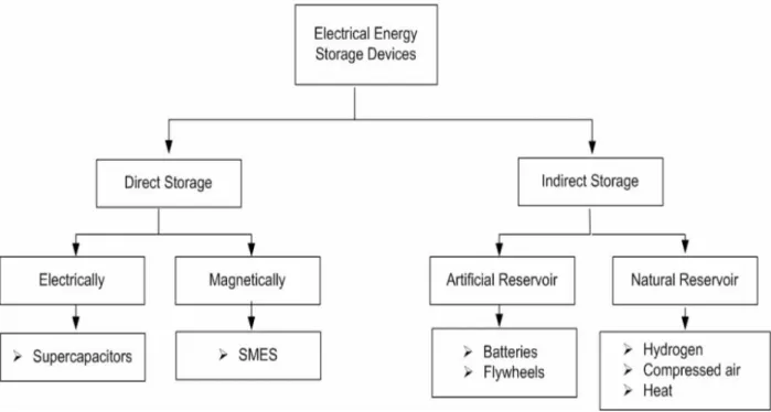
Therefore, storage systems can be divided in two main categories, and than subdivided into their specific storage reservoir. The next figure shows the main storage technologies and how they’re grouped together.

Figure 2.8: Electrical energy storage methods

Some of these technologies are intended for high power applications, some for low power, and others can be used on both. (i.e. batteries).

Modern man has witnessed the birth of the most diverse electronical equipment, some of which intended to be portable, and therefor “unplugged” from the power grid (PDA’s, laptops, mp3 players, ). A small, rechargeable and powerfull storage system is required, to provide the longest usage time between recharges.

The dominant energy storage technology for portable electronics are batteries. However batteries, like any other systems, have their cons. Their charging time is very long, have a short lifespan and are very sensitive to temperature. Other technologies are emerging and threatning to become a possible alternative to batteries. One of those emerging technologies are UC, which are already widely used as short term energy storage.

Both technologies will be presented in the next subsections, followed by a comparison and the conclusion over which technology to use for the project being developed.

2.2.1 Batteries

Batteries are electrochemical energy storage devices which convert chemical energy directly into electrical energy and vice-versa. They are formed by combining electrochemical cells of identical type in order to deliver higher voltage or current than a single cell. The battery cells create a voltage difference between the terminals of each cell, and hence, the bat-tery’s. When an external electrical circuit is connected to the battery’s terminals, a current is driven[13].

Figure 2.9: Various batteries with different shapes and voltages (taken from www.wikipedia.org)

The modern battery was invented in 1800 by Alessandro Volta and has become a popular power source for many household and industrial applications. There are both rechargeable and non rechargeable batteries. For this application the interest lies, of course, on the rechargeable ones, since the system is meant to be autonomous. The recharging process consists of applying an electric current to the battery, which reverses the chemical reactions that occured during it’s use.

All batteries are affected by self-discharge, meaning that even with no load applied, small chemical reactions occur, causing the battery to loose energy. The self-discharge rate is higher on rechargeable batteries than non-rechargeable.

Although rechargeable batteries may be refreshed by recharging, they still suffer degra-dation through usage. Normally a fast charge, rather than a slow overnight charge, will result in a shorter battery lifespan. However, if the overnight charger is not “smart” and can-not detect when the battery is fully charged, overcharging is likely, which will damage the battery[13]. By charging and discharging, the battery’s internal resistance increases until reaching unusable values.

Since the introduction, the battery development effort has been concentrated on extend-ing the capacity, increasextend-ing lifetime, minimizextend-ing self-discharge rate and increasextend-ing the power output while maintaining temperature stability, to mention some things[14].

The battery’s characteristics depend greatly on what type of chemical composition it is designed with. The following table resumes some characteristics of the most used recharge-able battery types in terms of cell voltage, energy and power density, self-discharge rate and cycle durability[15, 16, 17, 18]. Chemical composition Nominal cell voltage (V) Energy density (Wh/Kg) Power density (W/Kg) Self-discharge rate (month−1) Cycle durability NiCd 1.24 40-60 150 10% 2000 Lead Acid 2.105 30-40 180 3%-20% 500-800 NiMh 1.2 30-80 250-1000 30% 500-1000 Lithium ion 3.6/3.7 100-160 250-340 5%-10% 1200

Table 2.1: Battery types and characteristics

Lithium ion batteries are the ones with higher enery density, which means that they can supply an electronic circuit for a longer period than any of the other types. They also have a longer lifespan, around 1200 charge-discharge cycles. This lifespan is strongly dependent on working conditions, specially temperature. On avergage, for each 10ºC above optimum working temperature, a battery losses 10% lifespan.

One other problem affecting battery’s lifespan are incomplete charge/discharge cycles. The proper cycle should be taking the battery energy level from 90%/100% to 10%/20% dur-ing discharge and vice-versa durdur-ing charge. Chargdur-ing or dischargdur-ing batteries with interme-diate levels may decrease the total number of cycles before the battery becomes unusable. For the electronic water meter application in development, this is a huge drawback. Each time the HDG is activated (water starts flowing), the generated energy is conducted to the energy storage system, and when the HDG is inactive, energy is drawn from the storage to maintain the electronics. A full charge/discharge isn’t likely to happen. For this reason, a battery would have an even shorter lifespan.

Another huge drawback of batteries is to determine its SOC. To estimate the energy level, a reading of the output voltage must be made, and the SOC can be determined using the known discharge curve (voltage vs. SOC). However, the voltage is more significantly af-fected by the battery’s current (due to it’s internal resistance) and temperature. Furthermore, a correction term must be calculated, proporcional to the battery current and temperature. Readings of current and temperature must be obtained, and compared with a table of the battery’s Open Circuit Voltage Vs. Temperature. This adds up to some more electronics in the system, making it more expensive, complex, and less energetically efficient.

Since the HDG’s output varies with the water flow, charge control must be implemented. As it shown later on, the HDG is capable of supplying over 100mA of current. Since most batteries should be charged with around 10% of their nominal current, it would be necessary to use a 1A battery to absorb the energy produced by the HDG. That would be an oversized battery for a system that is estimated to consume a few miliamps. If a smaller battery is used, most of the HDG’s produced energy will be lost, with the risk of damaging the battery because of overcharging. This adds up to some more unnecessary complexity in the system.

2.2.2 Electric double-layer capacitors

Electric double-layer capacitors, also know as UC or SC, are electrochemical capacitors the have unsually high energy density when compared to common capacitors, typically on

the order of thousands of times greater than a high capacity electrolytic capacitor. As a comparison, a typical D-cell[19]sized electrolytic capacitor will have a capacitance in the range of tens of milifarads. The same size electric double-layer capacitor would have a capacitance of several farads, an improvement of about two or three orders of magnitude in capacitance, but usually at lower working voltage[20].

In a conventional capacitor, energy is stored by the removal of charge carriers, tipically electrons, from one metal plate and depositing them on another. This charge separation creates an electrical potential between the two plates, and a current will flow if connected to an external circuit.

Figure 2.10: Capacitor diagram (taken from www.wikipedia.org) The capacity is given by the formula C = E0×Er×A

d where:

• A - plate area [m2];

• d - distance between plates [m];

• E0- permittivity of free space = 8.854 x 10-12[F/m];

• Er- relative permittivity of the dielectric between the places [dimension less];

The capacity varies with the dielectric material between the plates, increases proportionally with the plate’s area and decreasses with the distance between them. Optimizing the mate-rials leads to higher energy densities for any given size of capacitor. However, the practical limitations on the surface area of the plates and the distance between the plates reduce capacitors’ ability to have the same high levels of capacitance found in UC.

UC solve this problem by using nanoporous materials, tipically activated carbon, that allows them to have enormous surface area relative to the distance between the plates. When two pieces of activated carbon are immersed into a liquid electrolyte, they form an amazingly effective capacitor. The success of this method is primarily due to the carbon’s large surface area-to-volume ratio, a product of the many microscopic nodules that cover its surface.

UC are made by coating two metal foil electrodes with this activated carbon, separating them with a thin piece of paper, and immersing the carbon-coated plates (the foil electrodes) into a liquid electrolyte.

The carbon on the negative plate collects electrons, which then attract positive ions from the electrolyte into the pores of the carbon. The carbon on the positive plate collects positive charges, which then attract negative ions from the electrolyte.

The thin piece of paper keeps the two plates from touching, which keeps the current from flowing between the two plates, allowing the positive and negative ions to move freely within their respective plates. This creates two layers of charge, making the ultracapacitor look like two capacitors in a series: this is the double-layer mechanism that gives ultracapacitors their name of "Electric Double-Layer Capacitors (EDLC)"

This design means that the charges on each plate of the ultracapacitor can be incredibly close to one another while still maintaining the carbon’s large surface area, giving ultraca-pacitors their high capacitance[21].

Figure 2.11: UC diagram (taken from www.wikipedia.org)

In terms of energy density, existing comercial UC range around 0.5 to 10 Wh/Kg. A group from MIT has demonstrated energy densities of 30 Wh/Kg and appear to be scalable to 60 Wh/Kg[22].

EEStor, a company from Texas, United States of America, claims to have developed a revolutionary new type of capacitor, with energy densities that could go over 250 Wh/Kg, intended to be used on electric cars. Many in industry have expressed great skepticism re-garding these claims. As a matter of fact, no prototypes have yet been publicly independently tested or acknowledge by anyone outside the company.

In terms of power density, UC have 10 to 100 times higher power density than bat-teries. This characteristic makes them the number one choice in applications where high amounts of energy need to be rapidly absorbed/released. They can be either discharged or charged very quickly without being damaged, and can withstand more than 500,000 charge/discharge cycles. In terms of duration, UC usually last up to 12 years.

They also present a very low internal series resistance, very high conversion efficiency (up to 98%), extremely low heating levels and are less affected by temperature. There are no disposable parts during the whole operating life of the device, which makes it environ-mentally friendly.

The main drawbacks from UC are the linear discharge voltage, preventing the use of the full energy spectrum; low energy density when compared to state of the art batteries; low

cell voltage, meaning that serial connections are needed to obtain higher voltages and cell ballancing must be implemented to prevent over charging; higher self-discharged rates than batteries.

Regarding the self-discharge rate, it is said to vary from 0.1% to 3% a day. A self dis-charge test was performed by charging a 2.7 100F to approximatelly full capacity and mea-suring it’s voltage during the course of 5 days. All the measurements were made at the same time of the day. The result is shown on table 2.2 .

Day Voltage (V) Energy (J) Daily self-discharge (%)

1 2.6860 360.73 0%

2 2.6672 355.70 1.39%

3 2.6457 349.99 1.6%

4 2.6284 345.42 1.30%

5 2.6109 340.84 1.33%

Table 2.2: Self discharge test

The UC tested averaged 1.40% of self-discharge a day. The self-discharge was calcu-lating based on the energy loss from one day to the following.

2.2.2.1 UC applications

The first ultracapacitor was developed by General Electric in 1957. The company used porous carbon electrodes to create the double-layer mechanism that characterizes ultraca-pacitors. The advantages of this mechanism weren’t fully understood until nearly a decade later, when the Standard Oil Company of Cleveland patented their double-layer interface energy storage device in 1966. Ultracapacitors’ first general use was as power, low-energy, long-life back-up power sources for consumer electronics such as VCRs. Today, UC are used with energy-storage and power-delivery functions in many different applications, which include:

• PC Cards

• flash photography devices in digital cameras • portable media players

• energy recovery • bridge power • motor start up

• electric vehicles in general

UC are becoming very attractive for the automotive industry. China has developed an electric bus that runs without power lines, using power stored on a large onboard array of UCs.

This energy storage can only power the bus for an average of three miles, but it recharges very quickly in every bus stop by an elevating system placed on top of each bus. This “elevator” makes contact with two charging poles located above each bus station which supply the energy for the recharge. A backup battery system ensures 15 more miles, in case the UC loose all their power.

Two commercial bus routes are already using these buses.

Figure 2.12: The UC bus at a bus stop (taken from www.youtube.com)

Honda’s hydrogen car also uses a large bank of ultra capacitors to supply short and high power bursts, during start up or acceleration. This hybrid battery/UC energy storage system uses the UC to buffer the batteries and protect them from high current demands, ensuring a longer lifespan.

Figure 2.13: Batteries/UC hybrid energy storage system (taken from www.afstrinity.com)

In addition, the UC are used to capture the energy generated during breaking, which would otherwise be lost in overheating. This technique is called regenerative breaking.

2.2.3 Choosing the energy storage system

After studying the characteristics of both batteries and UC, let us proceed with a comparison between them, in order to choose the most suitable solution.

The two following tables summarize the main pros and cons of batteries (in general) and UC:

Pros Cons

Widely used technology Temperature sensitive Relative high energy density Limited and controlled ROC

Flexibility Limited lifespan

Voltage is independente from SOC Limited charge/discharge cycles Relative low self-discharge Difficult SOC estimation

Table 2.3: Batteries pros and cons

Pros Cons

Over 500,000 charge/discharge cycles Relative low energy density

Very high ROC Voltage change with SOC

Easy SOC estimation Sensitive to overcharging High Power density Relative high self-discharge

Low internal resistance Low voltage

Table 2.4: UC pros and cons

The following graph resumes the difference between UC and batteries, when it comes to Energy and Power Density.

Figure 2.15: Energy and Power Density (taken from www.wikipedia.org) The key features of the energy storage system to be implemented should be:

• Long lifespan (or number of cycles), in order to eliminate the need of system mainte-nance;

• The ability to charge the device with least control as possible, so it can be connected to the HDG with the minimum charge interface electronics and absorb all the energy produced;

• Easy SOC estimation, also to make the system simpler both in terms of hardware and software;

High energy density isn’t a main characteristic, since the HDG will produce energy every time the water flows. Also, we don’t need high voltages (above 5V), since the system will be very low power, and most components are supplied by voltages from 2V to 5V. Since there are different working voltages for different components, there will be the need for some voltage regulators, hence, having a voltage that changes with SOC isn’t a problem.

The self-discharge should be the lowest possible. If the system looses its energy, there may be a period necessary for a minimum charge before the meter starts working.

2.2.3.1 Conclusion

From this short analysis, UC seem to be the right choice as an energy storage system. • They can be charged at any rate without being damaged, hence, no need for charge

control, which leads to system simplicity;

• SOC can be determined simply by measuring the output voltage of the UC and they are able to withstand over 500,00 charge/discharge cycles, which translates into years of use without the need of replacement;

• Number of charge/discharge cycles and overall lifespan will also increase the system’s lifespan;

• Higher self-discharge of UC can be a problem, but if the meter works on a daily basis, a few minutes of running water may be enough to compensate for that energy loss.

2.3

Hydro generation

2.3.1 History of hydro generation

Throughout history, people have always used water to their advantage. Romans had the aqueducts, the Egyptians were masters in irrigation methods, and around 200 B.C. the first water wheel was built. It converts the kinetic energy of the moving water into mechanical energy and was initially used to mill flour in watermills, but also had some other purposes such as foundry and machining, and later, hydro electricity. The first use of moving wa-ter to produce electricity was a wawa-ter wheel on the Fox River, Wisconsin, in 1882, which was shortly followed by a plant at the Niagara Falls[23]. It is estimated that hydroelectricity represents approximately 20% of the total worldwide electricity production and 88% when it comes to renewable sources[24]. Hydro generation can be divided into five main categories, according to their production capacity:

• Large Hydro: more than 10MW, usually supply energy for a few dozen small cities; • Small Hydro: between 10MW and 1MW, can supply a city or some industrial plants;

• Mini Hydro: between 1MW and 100KW, can supply a small community or small enter-prises;

• Micro Hydro: between 100KW and 5KW, can supply either a small community or a single household.

• Pico Hydro: less than 5KW, which can be enough to supply an entire household at least some of the home appliances.

Large Hydro Plants are usually located in big river streams, and the energy generated is then distributed to the surrounding area. As for all the other installations, tend to take advantage of smaller river streams, waterfalls, or any other source of running water. They also tend to be located as close as possible to the community/factory/house to be supplied, which guarantees a higher transport efficiency. Early hydroelectric power plants were much more reliable and effective than fossil fuel based power plants, which resulted in the proliferation of hydroelectric plants worldwide. In the middle of the 20th century, due to the increase of electricity demand and the incerasing efficiency of coal and oil fueled power plants, smaller hydroelectric plants fell out of favor. Nowadays, hydroelectric power plant projects are more focused in gigantic size plants, capable of producing more than 2000MW. The Three Gorges Dam in China is expected to reach 22500MW of electrical power production when it becomes fully operational in 2011. It’s located on the Yangtze River, and its construction began in December 1994[25].

2.3.2 The world’s smallest hydro generator

Vulcano is a sub holding company of the Bosch Group, specialized in the development and production of heating solutions, such as gas water heaters, central heating equipment and solar panels. In June 2000, Vulcano presented the world’s smallest hydro generator. Its purpose was to power up the automatic ignition and supply the electronics, instead of the common 9V batteries. Every time the hot water was turned on, the hydro generator’s rotation generated the energy required to the ignition process. This gave birth to a new gas water heater model, the Click HDG, which is energetically self-sustained, more ecologic, reliable and economic[26, 27]. The next figure shows the referedhydro generator.

Figure 2.17: Vulcano hydro generator (taken from www.vulcano.pt)

As the water passes through the hydro generator, there’s a small bypass that takes a part of that water and uses it to spin a rotor, which is no more than a cylindrical magnet. The magnet’s movement generates (by magnetic induction) a current in the stator (a circular winding) and a subsequent AC voltage in the output leads. The AC signal’s frequency and amplitude are proportional to the water flow, and therefore can be used as a flow measuring instrument.

To use the HDG as a flow measurement instrument, a mathematical relation must be established between either the frequency or the amplitude of the signal and the flow of water. In order to do so, a study of the HDG’s characteristics was performed.

It was connected to a hose so that the measures could be taken on real working condi-tions. Since there was no flowmeter available, the method used to measure the water flow was filling a half liter bottle and counting the filling time. From that value, and using a simple mathematical rule, the flow meter in liters per minute could be calculated.

2.3.3 Hydro generator study

2.3.3.1 AC characteristics

To have a mathematical model of the HDG, the first test consisted on measuring the output of the HDG (peak-to-peak voltage and frequency) using a digital oscilloscope. As previously mentioned, this test was performed in real conditions and with different running water flows. The output was left as an OC, with no load connected. The following graphs resulted from the measurements.

Figure 2.18: Frequency and peak-to-peak voltage Vs Water flow

It is clear the the HDG has a saturation point, where the increase of water flow doesn’t produce an increase of the output signal, neither in voltage nor frequency. That saturation point will be set at 2.5L/min. Another conclusion is that te HDG needs a minimum of 0.8 L/min of water flow to start opreating. Between 0.8 and 2.5 L/min, both voltage and fre-quency respond linearly to the water flow increase. This is a typical response of an AC generator.

The saturation is due to the size of the water bypass described earlier, and not to the generator’s physical properties, as it will be proved later on (with a DC motor simulating the water flow).

In order to find the mathematical relation between the water flow and the signals char-acteristics, the data was analyzed only on the linear response zone, ranging from 0.8 to 2.5 L/min. Using Matlab fitting tools, a linear fitting was performed on the data to obtain the mathematical equations that will be used.

Figure 2.19: Frequency and peak voltage Vs Water flow (up to 2.5 L/min)

From the fitting process resulted the two following equations:

• V = 4.5 × W F − 0.51, the relation between the WF and the output voltage (V in Volts and WF in L/min)

• F = 4.4e2_{× W F − 1.6e}2_{, the relation between the WF and the output frequency (F in}

Hz and WF in L/min)

These equations can be used to calculate the WF based on the readings of frequency and/or voltage.

2.3.3.2 Laboratory testing

Since no closed water circuit is available, a solution had to be found to use the HDG in laboratory. The solution consisted in disassembling an HDG and place a small DC motor to spin the rotor magnet. In fact, that solution was already available since the HDG was used in previous projects by the company Globaltronic, where this project was developed.

When using this setup to simulate the water flow, it was noticeable that for a given fre-quency, the peak-to-peak voltage was smaller than on the HDG used with running water. This could be caused by the following reasons:

• the HDG had not running water, therefor no cooling of the coil. An increasing temper-ature can affect the output voltage by decreasing it;

• also, this HDG has been extensively used on previous testing, so it must have some degree of degradation.

• it is also that the motor doesn’t exacly simulate the WF, an this causes a different output than the one obtained with water.

Also, the conclusion drawn from this observation is that the mathematical model that relates WF with output voltage cannot be used to in the reading method. The frequency Vs WF equation is the one to use in the water metering.

2.3.3.3 Power factor correction and maximum power transfer

In order to obtain the maximum output power, a power factor correction must be done. To do so, several capacitors were connected in parallel with the HDG’s output. Also, and to find the maximum power transfer point, several resistors were also placed, but separately from the capacitors. All the measurements were done with the same simulated water flow, so the motor used for the simulation was always supplied with the same voltage. This test will also allow for an estimation of the internal impedance of the HDG. The next graphs show the peak-to-peak voltage and RMS voltage for both the capacitors and the resistors test. The reason to measure the RMS is that the capacitors change the shape of the output signal from the HDG (which is originally a perfect sine wave).

The capacitor that gives the bigger boost to the the output voltage is the 12.5uF capacitor. Therefore, to conduct the resistos test, this capacitor was also placed in parallel with the output, in order to draw more power. Several resistors were connected and only the RMS voltage was measured, which was then used to calculate the power transferred to the resistor (P = V2/R).

Figure 2.21: Power transfer

The maximum transferred power is when the output resistor is between 20 to 25 ohm, more specifically, 21.7 ohm with 170 mW of transferred power. With this data, an estimation of the internal impedance of the HDG can be calculated. This is a representation of the circuit:

The internal impedance of the generator (Zg) is the R and L series and the impedance of the load applied (Zo) is the R and C parallel. It is known that for a maximum power transfer, Zo must be the conjugate of Zg. Assuming that C=12.5uF and R=21.7ohm are the values corresponding to the maximum power transfer, the parallel model for the load must be converted into the series model:

Figure 2.23: Equivalent circuit with series load impedance

After converting from the parallel to the series model, the new values for R and C are R=6.48 and C=17.8uF, thus the internal R=6.48 and internal L=1.7mH.

To charge an UC using the HDG, the signal must be rectified. To do so, a diode bridge was inserted, and several capacitors were connected parallel with the output of the HDG. No load was placed after the rectifier. It is assumed that HDG generates more energy with a correction capacitor, because of the voltage boost.

Figure 2.24: Output capacitors

Now it can be observed that the capacitor that gives the output voltage the bigger boost is the 1uF, and thus, a different capacitor from the previous test. The RMS voltage was measured at the output of the rectifier circuit with no load connected. At this point, the decision was made to use the 1uF capacitor as the power factor correction capacitor.

Since the purpose of the HDG is to charge an UC, the final test was charging a 100F 2.5V UC with the HDG. The ultra cap was connected directly to the output of the rectifier, so it could drain a high current in the initial charging stage. Measures of current and voltages (HDG’s peak-to-peak voltage and UC voltage) were taken every 30 seconds. To measure the current a 1ohm resistor was placed in series with the UC. The HDG’s rotation was kept constant during this test with a value of 800Hz.

Figure 2.25: Ultra cap charging

As expected, the ultra cap reveals a logarithmic charging behavior, also because it is charged with a variable current. Both the output peak voltage of the HDG and the charging current vary throughout the charging test, which was also expected, since the HDG voltage is limited by the UC voltage. The initial current was 120mA an dropped to 30mA after 40min of continuous charging.

If a single hydro generator is used in a household, with family of four, and assuming that everyone takes a 10 min bath ever day, the produced electrical energy would be enough to charge one ultra cap up to 2V. Additional water usage (for laundry or dish washing) would even increase the charge on the ultra cap.

Chapter 3

UC CHARGING AND SOC

MONITORING SYSTEM

3.1

Introduction

It is a well known fact that battery chargers can be quite complex, both in terms of hard-ware and softhard-ware. They must have current, voltage and temperature control, in order to charge the batteries without causing damage. As a first approach to UC based electronics, a charging and monitoring system was developed. It is based on a Microchip microcon-troller (PIC18F14K50) which reads and converts current and voltage values. Those values are then sent, to a computer, using an RS-232 interface. The computer later processes and presents the data in a graphical interface developed in C#. Charging current, UC voltage and energy level are shown in a friendly and easy to read manner. To make communication possible between the microcontroller and the computer, a device was used to convert be-tween TTL/CMOS levels and RS-232 levels which is this case was an SP232ACP. For the results displayed, a 100F 2.5V UC was used

3.2

HDG and rectifying bridge

The HDG is an AC voltage generator, and therefor becomes imperative have a rectifier. The rectifier implemented was a textbook classic full-wave rectifier. In paralell with the output was palced the power factor correction capacitor followed by the bridge, formed by four low-drop diodes. Between the bridge and the 100F UC, a 1ohm resistor was placed to make current readings.

Figure 3.1: HDG and rectifying diode bridge

Before using the 1uF capacitor, the ouput was an almost perfect, noise free AC voltage signal. After placing the capacitor for power factor correction, the output changed in shape and peak voltage (which increased).

Figure 3.2: HDG output with paralell 1uF capacitor and no load

After connecting the remaining hardware (bridge, resistor and UC), the output changed to a square shaped signal.

Figure 3.3: HDG output with connected circuit

This is caused by the simple fact that the UC limits the peak voltage. This limitation is translated into current flowing from the HDG to the UC charging it. The current varies according with the SOC of the UC. The lower the UC’s SOC, the lower the HDG’s voltage, and the higher the charging current.

3.3

Microcontroller

The microcontroller is a simple PIC18F14K50. It was initially choosen due to its wide range supply voltage(1.8- 5V) and low-power features, which would be important for the electronic water meter. Pin count on this device (20) wasn’t taken into account, and revealed insuffi-cient, being later replaced by another model (18LF2520).

Figure 3.4: Microcontroller

It is supplied by a 5V voltage regulator (7508) and an external power source. The 5V DC is also used as the V+ ADC voltage reference.

Measures of voltage are taken before and after the 1ohm resistor (output of the diode bridge and UC) on analog channels 9 and 6 respectivelly. All the other data is determined based on these two measures. Furthermore, charge current is the voltage drop on the 1ohm resistor (V/R, R=1) and SOC of the UC (or energy level) is determined by the formula

1

2 × C × V

2_{, where V is the UC’s voltage. These mathematical operations are performed on}

the computer. The software on the microcontroller has a very simple flow.

Figure 3.5: Software fluxogram

Voltage readings are taken on channels 6 and 9, formatted to a previously determined format and sent threw a serial communication protocol to a computer for processing.

The choosen format is a string formed by 8 characters. The first 4 characters are the voltage of the UC and the following 4 characters are the voltage at the output of the diode bridge. Both are in milivolt units.

3.4

Graphical user interface

The GUI for this system was developed in C#, using Visual Studio C# express. C# is in-tended to be a simple, modern, general-purpose, object-oriented programming language. Visual Studio’s IDEhas embedded functions for serial port management, such as port open-ing, buffer checking and readopen-ing, among others. The final aspect of the developed GUI is shown in the next image.

Figure 3.6: Graphical user interface

The user must insert the UC’s capacity and maximum voltage, in order for the system to determine the SOC correctly. On the first bar below the Start button charge percentage and energy are presented, and the second bar is filled (from left to right) according with that percentage. The following three bars are used to display charge current, UC’s voltage and bridge output voltage.

The fluxogram for this small software is as follows.

Figure 3.7: Graphical user interface software fluxogram

The user beings by entering values for the UC’s capacity and maximum allowed voltage. The software will not read those fields while the user doesn’t press the Start button. When

Start button is pressed, the values are read and the software beings a cycle where it checks if the buffer has the 8 expected bytes. When the buffer is filled with the 8 bytes, the data is read, processed and displayed as previously explained.

3.5

Conclusion

In this chapter was shown how the SOC of an UC can be determined. With simple hard-ware and softhard-ware, an accurate SOC determination can be performed and displayed, in this case, in a graphical form. Another conclusion extracted is that the mathematical equation obtained on subsubsection 2.3.3.1 which relates the HDG’s voltage with the water flow can-not be used. This dues to the fact that the voltage varies when the HDG is connected to a closed circuit, or in this case, to a rectifying diode bridge with an UC. For the water metering process, the frequency and its associated equation is the signal characteristic that must be used.

Chapter 4

WATER METER PROJECT

-HARDWARE

4.1

Introduction

The electronic water meter is formed by four main hardware blocks: • HDG, rectifying diode bridge and two UC (100F 2.7V);

• Microcontroller unit and surrounding electronic; • LCD;

• GSM modem.

The HDG is the energy generator for all the electronics, and also the measurement instru-ment. It’s a simple AC generator with an inductor (stator) and a magnet (rotor) that is spinned by the running water. Using the rectifying bridge, the output power of the HDG is used to charge two UC, which will be the only energy storage unit. The option of using two UCs instead of one was to extend the systems lifespan and avoid the use of step up converters which would drain the UCs rapidly. The choosen microcontroller was a PIC18LF2520 from Microchip. This model was chosen because of it’s lowpower features (Microchip’s nanoWatt technology) and wide operating voltage range (2 - 5.5V). This characteristic allows for the microcontroller to be connected directly to the terminals of the UCs without any voltage regulation, diminishing energy losses.

The LCD unit will be used for local readings. A button must be pressed by the user when he wishes to make a reading, and the system will display the data on the LCD for a period of about 5 seconds. This is considered to be enough for the user to memorize the reading and is almost irrelevant in terms of energy consumption.

For remote readings, a GSM module was placed, which sends an SMS with updated readings.

Both the LCD and GSM require different supply levels, 5V and 3.8V respectfully. This implies the introduction of two voltage regulators, to ensure proper device operation. Also, and once again because of the variable supply voltage of the microcontroller, a level shifter was needed to ensure the communication between the GSM module and the microcontroller using USART interface.

4.2

Energy storage

It was initially intended to use one single UC, but that would implie using voltage regulation. Using two UCs directly connected to the microcontroller (which is the only IC that is always active), we eliminate the need for voltage regulations. The chosen UCs are 100F 2.7V, that corresponds to one single 50F 5.4V UC (two equal capacitors in series are equivalent to one capacitor with have half the capacity). Fully charged we have a total of 729J of energy stored (1₂ × 50 × 5.42_{). For the system to remain operational (except for the GSM module)}

and able to perform water metering, the minimum allowed voltage is 2V, which corresponds to the minimum supply voltage of the microcontroller. Therefore 100J of energy (1₂× 50 × 22₎

will remain stored in the UCs. This means that the storage system can transfer 86.3% of its energy to the electronic system (not accounting for self-discharge). The remaining 13.7% can’t be transfered to the system with the chosen configuration (directly connected) and a boost converter is necessary to extract that remaining energy if necessary.

Figure 4.1: HDG, diode bridge and UCs schematic

Figure 4.1 shows the orcad schematic of the power source/storage block. As previously explained, the HDG’s AC signal is rectified and charges two UCs. Due to the it’s inductive characteristic, the output is boosted by a 1uF power factor correction capacitor. This value was obtained empirically and is detailed on section 2.3. The net PIC_VDD connects directly to the microcontroller and contains a DC voltage from the UCs. To measure the water flow rate we must use the AC signal directly from the HDG’s output and measure it’s frequency. So a connection was done between one of the outputs and a pin of the microcontroller. Details on this connection and measuring algorithm will be given at a later section.

It it common to use regulation on the UCs so they don’t overcharge. In this case, no regulation is necessary due to the fact that the HDG has a peak voltage limited to around 11V. Therefore, the UCs voltage will never be much higher than 5.2V: 11V divided by two (from the rectifier) minus the drop on two diodes (around 0.15V each).

4.3

LCD

Figure 4.2: LCD

The typical supply voltage for the LCD is 5V, but can vary +/- 10% (from 4.5 to 5.5V)[28]. Since the power supply, hence, the UCs can vary from 5.2V to 2V, it is imperative to imple-ment a regulator (with step up characteristics) to give the LCD a steady DC supply. For this porpuse, an IC from Texas Instruments was chosen (TPS61200), because it can regulate 5V even with low inputs (down to 0.5V)[29]. This regulator is only available in a QFN package which is very small and hard to mount[30]. A small PCB board was done to test the device but due to the components size it wasn’t possible to make it work. So the alternative was to get an evaluation module for this component (TPS6120x-EVM) which solved this problem for the prototype development.

Figure 4.3: 5V Regulator

On the input of the regulator the voltage of the power source is applied to obtain a steady 5V regulated voltage on the output. In order to shutdown the device, a pull-down resistor was connected between enable pin and ground. The enable is active high, meaning that a signal equal to Vdd must be applied on this pin to turn on the regulator. Most of the time it is to remain off, only to be activated if the user requests a local reading, hence the LCD must be turned on.

Figure 4.4: LCD schematic

On figure 4.4 the schematic of the LCD is shown. Pin 11 to 14 are data pins used to write and read data. Pin 4 is the register selection pin, indicating if we want to access instructions or data registers. Pin 5 is used to signal if the operation will be read (active high) or write (active low). Next, there is a pin to activate or deactivate the LCD (pin 6) which must be used in some situations. On pins 16 and 2 DC voltage supply is applied and Ground is connected to pins 1 and 15. To adjust contrast, a pontentiometer is connected between 5V and ground, with the middle point connected to pin 3. Pins 7 to 10 are not used in this case, since communication can be established between the LCD and the microcontroller by using only 4 data pins.

The LCD acknowledges high voltage levels starting from 0.7Vdd, hence, over 3.5V. If the UCs voltage drops below that value, it is possible that the LCD doesn’t not work properly.

4.4

GSM modem

For remote data transmission, SMS texting seemed the wisest choice, since the user can be virtually anywhere on the planet and still receive an sms with meter readings. Other technologies were pondered such as bluetooth or zigbee, but were dropped out due to their limited range. The modem of option was a GC864 from Telit.

Figure 4.6: GC864 bottom view

This modem must be supplied with 3.8V, and similiar to the LCD, a regulator was in-serted in the circuit. When transmiting, the modem sends bursts at a base frequency of about 216Hz, where current peaks can be as high as 2A[31]. Because of this current de-mand, and as precaution, the regulator chosen was a TPS7580 from Texas Instruments. It is a 3A LDO regulator with adjustable output voltage[32]. This way the regulator oper-ates in a voltage safe-zone, prevents overheating or high voltage drops during transmission. During the first tests with the modem, sometimes the modem was doing a reset every 4 or 5 seconds. Later it was observed that it only happened with the antena connected. The conclusion was obvious: when the modem had the antenna connected it tried to establish communication with the mobile network. In order to do so, it had to make burst transmission, which demanded high current peaks. Despite being able to respond to those current peaks, the regulator suffered a voltage drop that caused the modem to reset. The problem was only solved by placing a parallel 1000uF capacitor with the output of the regulator to prevent this voltage drop.

Figure 4.7: GSM modem schematic

The 3.8V regulator also has an enable pin, controlled by the microcontroller. This way we have total control over it, and it remains off during most of the time to ensure minimum current leaks. Also in this case, a pull down resistor was applied between the pin and ground.