CERN-PH-EP/2015-211 2016/04/28
CMS-HIG-14-034
Searches for a heavy scalar boson H decaying to a pair of
125 GeV Higgs bosons hh or for a heavy pseudoscalar
boson A decaying to Zh, in the final states with h
→
ττ
The CMS Collaboration
∗Abstract
A search for a heavy scalar boson H decaying into a pair of lighter standard-model-like 125 GeV Higgs bosons h and a search for a heavy pseudoscalar boson A decaying into a Z and an h boson are presented. The searches are performed on a dataset corresponding to an integrated luminosity of 19.7 fb−1of pp collision data at a centre-of-mass energy of 8 TeV, collected by CMS in 2012. A final state consisting of two τ leptons and two b jets is used to search for the H→hh decay. A final state consisting of two τ leptons from the h boson decay, and two additional leptons from the Z boson decay, is used to search for the decay A → Zh. The results are interpreted in the context of two-Higgs-doublet models. No excess is found above the standard model expectation and upper limits are set on the heavy boson production cross sections in the mass ranges 260<mH<350 GeV and 220<mA <350 GeV.
Published in Physics Letters B as doi:10.1016/j.physletb.2016.01.056.
c
2016 CERN for the benefit of the CMS Collaboration. CC-BY-3.0 license
∗See Appendix B for the list of collaboration members
1
Introduction
The discovery of additional Higgs bosons at the LHC would provide direct evidence of physics beyond the standard model (SM). There are several types of models that require two Higgs doublets [1–3]. For example the minimal supersymmetric extension of the SM (MSSM) requires the introduction of an additional Higgs doublet, where one Higgs doublet couples to up-type quarks and the other to down-type quarks [4–11]. This leads to the prediction of five Higgs particles: one light and one heavy CP-even Higgs boson, h and H, one CP-odd Higgs boson A, and two charged Higgs bosons H± [2, 12]. The masses and couplings of these bosons are interrelated and, at tree level, can be described by two parameters, which are often chosen to be the mass of the pseudoscalar boson mA and the ratio of the vacuum expectation values of the neutral components of the two Higgs doublets tan β. However, radiative corrections [13–17] introduce dependencies on other parameters namely the mass of the top quark mt, the scale of the soft supersymmetry breaking masses MSUSY, the higgsino mass parameter µ, the wino mass parameter M2, the third-generation trilinear couplings, At, Ab, and Aτ, the mass of the
gluino meg, and the third-generation slepton mass parameter M˜`3.
Direct searches for the neutral MSSM Higgs bosons have been performed by the CMS and ATLAS Collaborations [18–20] using the benchmark scenarios proposed in Ref. [21]. In these scenarios the parameters involved in the radiative corrections for the Higgs boson masses and couplings have been fixed, and only the two parameters mAand tan β remain free. The value of MSUSYwas fixed at around 1 TeV, which produces a lightest CP-even Higgs boson with a mass mhlower than the observed Higgs boson mass of 125.09±0.21 (stat)±0.11 (syst) GeV [22], for values of tan β.6.
If, however, MSUSYis much larger than 1 TeV, as suggested by the non-observations of SUSY partner particles at the LHC so far, low values of tan β can produce an h boson with mh ' 125 GeV [23, 24]. The interpretation of the Higgs boson measurements in the framework of the recently developed MSSM benchmark scenarios [24–27] suggests that the mass of the CP-odd Higgs boson, mA, can be smaller than 2mt. In the mass region below 2mtand at low values of tan β, the decay mode of the heavy scalar H → hh and that of the pseudoscalar A → Zh can have sizeable branching fractions.
This encourages a programme of searches in the so-called “low tan β” channels [23, 28]: • for 220 GeV<mA <2mt: A→Zh;
• for 260 GeV<mA <2mt: H→hh; • for mA >2mt: A/H→tt.
The decay modes H→ hh and A → Zh, studied in this paper, are also present in other types of two-Higgs-doublet models (2HDM) [2, 3]. There are different types of 2HDM with those most similar to the MSSM ( i.e. where up-type fermions couple to one doublet and down-type fermions to the other) being “Type II” 2HDM. The discovery of a Higgs boson at the LHC [29–31] with a mass around 125 GeV pushes the 2HDM parameter space towards either the alignment or decoupling limits [24]. In these limits the properties of h are SM-like.
In the alignment limit of 2HDM when cos(β−α) 1 (where α is the mixing angle between the two neutral scalar fields), the Hhh and AZh couplings vanish at Born level [32]. However, in the MSSM, the Hhh and AZh couplings do not vanish, even in the alignment limit, because of the large radiative corrections that arise in the model. In the decoupling limit of 2HDM the scalar Higgs boson H has a very large mass and the decay H→tt dominates [32].
h h h h h
visible products of a hadronically decaying τ, whereas for the channel A → Zh → ``ττ, the µτh, eτh, τhτh, and eµ final states are selected.
Searches for the decays H→hh, and A→Zh have already been performed by the ATLAS [35– 38] and CMS Collaborations [39–41] in di-photon, multilepton and bb final states.
This analysis has the power to bring important results in the low tan β region for the mArange, which has been previously discussed and where these processes have an enhanced sensitiv-ity [23]. This region has not yet been excluded by the direct or indirect searches for a heavy scalar or pseudoscalar Higgs boson, that have been mentioned above, therefore the described decay modes look to be quite promising.
For simplicity of the paper, we are neither indicating the charge of the leptons nor the particle-antiparticle nature of quarks.
2
The CMS detector, simulation and data samples
A detailed description of the CMS detector can be found in Ref. [42]. The central feature of the CMS apparatus is a superconducting solenoid of 6 m internal diameter providing a field of 3.8 T. Within the field volume are a silicon pixel and strip tracker, a crystal electromagnetic calorimeter (ECAL), and a brass/scintillator hadron calorimeter. Muons are measured in gas-ionisation detectors embedded in the steel return yoke of the magnet.
The CMS coordinate system has the origin centered at the nominal collision point and is ori-ented such that the x-axis points to the center of the LHC ring, the y-axis points vertically upward and the z-axis is in the direction of the beam. The azimuthal angle φ is measured from the x-axis in the xy plane and the radial coordinate in this plane is denoted by r. The polar angle θ is defined in the rz plane and the pseudorapidity is η = −ln[tan(θ/2)][42]. The mo-mentum component transverse to the beam direction, denoted by pT, is computed from the x− and y−components.
The first level (L1) of the CMS trigger system, composed of custom hardware processors, uses information from the calorimeters and muon detectors to select the most interesting events in a fixed time interval of less than 4 µs. The high-level Trigger processor farm decreases the L1 accept rate from around 100 kHz to less than 1 kHz before data storage.
The data used for this search were recorded with the CMS detector in proton-proton collisions at the CERN LHC and correspond to an integrated luminosity of 19.7 fb−1 at a centre-of-mass energy of √s = 8 TeV. The H → hh signals are modelled with the PYTHIA 6.4.26 [43] event
generator while the A → Zh signals were modelled with MADGRAPH 5.1 [44]. When
mod-elling background processes, the MADGRAPH 5.1 generator is used for Z+jets, W+jets, tt, and
diboson production, and POWHEG1.0 [45–48] for single top quark production. The POWHEG
and MADGRAPHgenerators are interfaced withPYTHIAfor parton showering and fragmenta-tion using the Z2* tune [49]. All generators are interfaced withTAUOLA[50] for the simulation of the τ decays. All generated events are processed through a detailed simulation of the CMS detector based on GEANT4 [51] and are reconstructed with the same algorithms as the data. Parton distribution functions (PDFs) CT10 [52] or CTEQ6L1 [53] for the proton are used,
de-pending on the generator in question, together with MSTW2008 [54] according to PDF4LHC prescriptions [55].
3
Event reconstruction
During the 2012 LHC run there were an average of 21 proton-proton interactions per bunch crossing. The collision vertex that maximizes the sum of the squares of momenta components perpendicular to the beamline (transverse momenta) of all tracks associated with it, ∑ p2T, is taken to be the vertex of the primary hard interaction. The other vertices are categorised as pileup vertices.
A particle-flow algorithm [56, 57] is used to reconstruct individual particles, i.e. muons, elec-trons, photons, charged hadrons and neutral hadrons, using information from all CMS subde-tectors. Composite objects such as jets, hadronically decaying τ leptons, and missing transverse energy are then constructed using the lists of individual particles.
Muons are reconstructed by performing a simultaneous global track fit to hits in the silicon tracker and the muon system [58]. Electrons are reconstructed from clusters of ECAL energy deposits matched to hits in the silicon tracker [59]. Muons and electrons assumed to originate from W or Z boson decays are required to be spatially isolated from other particles [59, 60]. The presence of charged and neutral particles from pileup vertices is taken into account in the isolation requirement of both muons and electrons. Muon and electron identification and isolation efficiencies are measured via the tag-and-probe technique [61] using inclusive samples of Z → `` events from data and simulation. Correction factors are applied to account for differences between data and simulation.
Jets are reconstructed from all particles using the anti-kT jet clustering algorithm implemented inFASTJET[62, 63] with a distance parameter of 0.5. The contribution to the jet energy from
par-ticles originating from pileup vertices is removed following a procedure based on the effective jet area described in Ref. [64]. Furthermore, jet energy corrections are applied as a function of jet pT and η correcting jet energies to the generator level response of the jet, on average. Jets originating from pileup interactions are removed by a multivariate pileup jet identification algorithm [65].
The missing transverse momentum vector~pmiss
T is defined as the negative vector sum of the transverse momenta of all reconstructed particles in the volume of the detector (electrons, muons, photons, and hadrons). Its magnitude is referred to as ETmiss. The ETmiss reconstruc-tion is improved by taking into account the jet energy scale correcreconstruc-tions and the φ modulareconstruc-tion, due to collisions not being at the nominal centre of CMS [66]. A multivariate regression correc-tion of EmissT , where the contributing particles are separated into those coming from the primary vertex and those that are not, mitigates the effect of pileup [66].
Jets from the hadronisation of b-quarks (b jets) are identified with the combined secondary vertex (CSV) b tagging algorithm [67], which exploits the information on the decay vertices of long-lived mesons and the transverse impact parameter measurements of charged particles. This information is combined in a likelihood discriminant. The medium value of the CSV discriminator, corresponding to a b jet misidentification probability of 1%, has been used in this analysis.
Hadronically decaying τ leptons are reconstructed using the hadron-plus-strips algorithm [68], which considers candidates with one charged pion and up to two neutral pions, or three charged pions. The neutral pions are reconstructed as “strips” of electromagnetic particles
4
Event selection
The events are selected with a combination of electron, muon and τ trigger objects [34, 59, 60, 69]. The identification criteria of these objects were progressively tightened and their transverse momentum thresholds raised as the LHC instantaneous luminosity increased over the data taking period. A tag-and-probe method was used to measure the efficiencies of these triggers in data and simulation, and correction factors are applied to the simulation.
Electrons, muons, and τhare selected using the criteria defined in the CMS search for the SM Higgs boson at 125 GeV [34]. Specific requirements for the selection of the H → hh → bbττ and the A→Zh→ ``ττchannels are described below.
4.1 Event selection of H
→
hh→
bbττIn the H→hh→bbττ channel, the three most sensitive final states are analysed, distinguished by the decay mode of the two τ leptons originating from the h boson (µτh, eτhand τhτh). In the µτhand eτhfinal states, events are selected with a muon with pT >20 GeV and|η| <2.1 or an electron of pT > 24 GeV and |η| < 2.1, and an oppositely charged τh of pT > 20 GeV and|η| <2.3. To reduce the Z→µµ, ee contamination, events with two muons or electrons of pT >15 GeV, of opposite charges, and passing loose isolation criteria are rejected.
In the µτhand eτhfinal states, the transverse mass of the muon or electron and~pmiss T mT =
q
2pTEmissT (1−cos∆φ), (1)
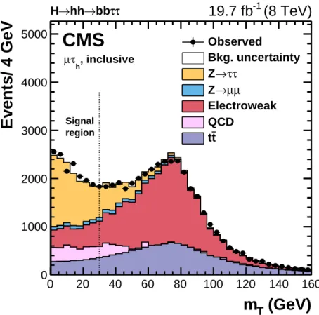
where pT is the lepton transverse momentum and∆φ is the difference in the azimuthal angle between the lepton momentum and~pmissT , is required to be less than 30 GeV to reject events coming from W+jets and tt backgrounds. The mT distribution for the µτh final state is shown in Fig. 1.
In the τhτhfinal state, events with two oppositely charged hadronically decaying τ leptons with pT >45 GeV and|η| <2.1 are selected.
In addition to the ττ selection, each selected event must contain at least two jets with pT > 20 GeV and |η| < 2.4. These pT and η requirements are necessary to select jets that have a well defined value of the CSV discriminator (Section 3), which is important for categorising signal-like events with two b jet candidates coming from the 125 GeV Higgs boson decaying to bb.
Simulation studies show that the majority of signal events will have at least one jet passing the medium working point of the CSV discriminator. The jets are ordered by CSV discriminator value, such that the leading and subleading jets are defined as those with the two highest CSV values. Then the events are separated into categories, defined as:
• 2jet–0tag when neither the leading nor subleading jets passes the medium CSV work-ing point. Only a small amount of signal is collected in this category, which is background-dominated.
(GeV)
Tm
0 20 40 60 80 100 120 140 160Events/ 4 GeV
0 1000 2000 3000 4000 5000 τ τ bb → hh → H , inclusive h τ µ region Signal Observed Bkg. uncertainty τ τ → Z µ µ → Z Electroweak QCD t tCMS
(8 TeV)
-119.7 fb
Figure 1: Distribution of mTfor events in the µτhfinal state, containing at least two additional jets. The W+jets background is included in the “electroweak” category. Multijet events are indicated as QCD. The H → hh → bbττ selection requires mT < 30 GeV for the µτhand eτh final states.
• 2jet–1tag when only the leading but not the subleading jet passes the medium CSV working point.
• 2jet–2tag when both the leading and subleading jets pass the medium CSV working point.
The signal extraction is performed using the distribution of the reconstructed mass of the H boson candidate.
4.2 Event selection of A
→
Zh→ ``
ττIn the A→Zh→ ``ττchannel eight final states are analysed. These are categorised according to the decay mode of the Z boson and the decay mode of the τ leptons originating from the h boson.
The Z boson is reconstructed from two same-flavour, isolated, and oppositely charged electrons or muons. In the Z → µµ(ee) final state the muons (electrons) are required to have|η| < 2.4 (2.5) with pT >20 GeV for the leading lepton and pT > 10 GeV for the subleading lepton. The invariant mass of the two leptons is required to be between 60 GeV and 120 GeV. When more than one pair of leptons satisfy these criteria, the pair with an invariant mass closest to the Z boson mass is selected.
After the Z candidate has been chosen, the h → ττdecay is selected by combining the decay products of the two τ leptons in the four final states µτh, eτh, τhτh, eµ. The combination of the
these requirements are rejected.
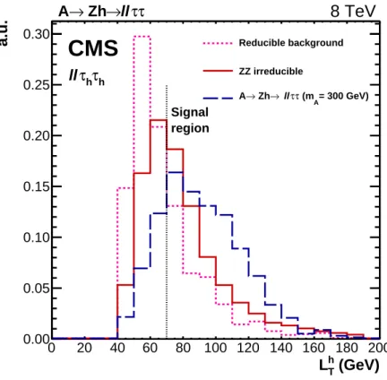
A requirement on LhT, which is the scalar sum of the visible transverse momenta of the two τ candidates originating from the h boson, is applied to lower the reducible background from misidentified leptons as well as the irreducible background from ZZ production. The thresh-olds of this requirement depend on the final state and have been chosen in such a way as to optimise the sensitivity of the analysis to the presence of an A → Zh signal for A masses be-tween 220 and 350 GeV. The distribution of LhTfor events in the``τhτhfinal state can be seen in Fig. 2. (GeV) h T L 0 20 40 60 80 100 120 140 160 180 200 a.u. 0.00 0.05 0.10 0.15 0.20 0.25 0.30 Reducible background ZZ irreducible = 300 GeV) A (m τ τ ll → Zh → A
8 TeV
CMS
h τ h τ ll τ τ ll → Zh → A region SignalFigure 2: Distribution of the variable LhT for events in the ``τhτh final state. The reducible background is estimated from data, instead the ZZ irreducible background from simulation. In order to reduce the tt background, events containing a jet with pT > 20 GeV,|η| < 2.4 and passing the medium working point of the CSV b tagging discriminator are removed.
The four final objects are further required to be separated from each other by∆R= √
(∆η)2+ (∆ϕ)2 larger than 0.5 (where phi is in radians), and to come from the same primary vertex.
In this channel the signal extraction is performed using the distribution of the reconstructed mass of the A boson candidate.
5
Background estimation
5.1 Background estimation for H
→
hh→
bbττThe backgrounds to the H → hh → bbττ final state consist predominantly of tt events, fol-lowed by Z → ττ+jets events, W+jets events, and QCD multijet events, with other small con-tributions from Z→ ``, diboson, and single top quark production. The estimation of the shapes of the reconstructed H mass and of the yields of the major backgrounds is obtained from data wherever possible.
The Z→ ττprocess constitutes an irreducible background due to its final state involving two τ leptons, which only differ from the h → ττ signal by having an invariant mass closer to the mass of the Z boson instead of the Higgs boson. Requiring two jets in the event greatly reduces this background and the b tagging requirements reduce it even further. Nevertheless, it still remains an important source of background events, in particular in the 2jet–1tag and 2jet–0tag categories. This background is estimated using a sample of Z → µµ events from data, obtained by requiring two oppositely charged isolated muons, where the reconstructed muons are replaced by the reconstructed particles from simulated τ decays. A correction for a contamination from tt events is applied to the Z → µµselection. This technique substantially reduces the systematic uncertainties due to the jet energy scale and the missing transverse energy, as these quantities are modelled with data.
For the tt background, both shape and normalisation are taken from Monte Carlo simulation (MC), and the results are checked against data in a control region where the presence of tt events is enhanced by requiring eµ in the final state instead of a ditau, and at least one b tagged jet.
Another significant source of background is from QCD multijet events, which can mimic the signal in various ways, e.g. where one or more jets are misidentified as τh. In the µτhand eτh channels, the shape of the QCD background is estimated using an observed sample of same-sign (SS) ττ events. The yield is obtained by scaling the observed number of SS events by the ratio of the opposite-sign (OS) to SS event yields obtained in a QCD-enriched region with relaxed lepton isolation. In the τhτhchannel, the shape is obtained from OS events with relaxed τisolation. The yield is obtained by scaling these events by the ratio of SS events with tighter and relaxed τ isolation.
In the µτh and eτh channels, W+jets events in which there is a jet misidentified as a τh are another sizeable source of background. The W+jets shape is modelled using MC simulation and the yield is estimated using a control region of events with large mT close to the W mass. In the τhτhchannel this background has been found to be less relevant and its shape and yield are taken from MC simulation.
The contribution of Drell–Yan production of muon and electron pairs is estimated from simu-lation after rescaling the simulated yield to that measured from observed Z → µµ events. In the eτhchannel, the Z→ ee simulation is further corrected using the e→ τhmisidentification rate measured in data using a tag-and-probe technique [61] on Z→ee events.
Finally the contributions of other minor backgrounds such as diboson and single top quark events are estimated from simulation. Possible contributions from SM Higgs boson production are estimated and found to have a negligible effect on the final result.
the same final states as the expected signal. Other “rare” sources of irreducible background are SM Higgs boson associated production with a Z boson, ttZ production where the Z boson decays into a muon or an electron pair and both top quarks decay leptonically (to e, µ, or τh), and triboson events (WWZ, WZZ, ZZZ). The contributions of all the irreducible backgrounds after the final selection are estimated from simulation.
The reducible backgrounds have at least one lepton in the final state that is due to a misiden-tified jet that passes the lepton identification. In``τhτhfinal states, the reducible background is essentially composed of Z+jets events with at least two jets, whereas in``µτhand``eτhfinal states, the main contribution to the reducible background comes from WZ+jets with three light leptons. The contribution from these processes to the final selected events is estimated using control samples in data.
The probabilities for a jet that passes relaxed lepton selection criteria to pass the final identi-fication and isolation criteria of electrons, muons, and τ leptons are measured in a signal-free region as a function of the transverse momentum of the object closest to the candidate, f(pfakeT ). In this region, events are required to pass all the final state selections, except that the recon-structed τ candidates are required to have the same sign and to pass relaxed identification and isolation criteria. This effectively eliminates any possible signal, while maintaining roughly the same proportion of reducible background events.
In order to use the misidentification probabilities f(pfakeT ), sidebands are defined for each chan-nel, where, unlike the relaxed criterion, the final identification or isolation criterion is not satis-fied for one or more of the final state lepton candidates. The number of reducible background events due to a lepton being misidentified in the final selection is estimated by applying the weight f(pfake
T )/(1− f(pfakeT ))to the observed events with lepton candidates in the sideband that satisfy the relaxed but not the final identification or isolation criterion. Finally, the re-ducible background shape of the reconstructed A mass is obtained from a SS signal–free region where the τ candidates have the same charge and relaxed isolation criteria. Possible contribu-tions from SM Higgs boson production are estimated and found to have a negligible effect on the final result.
6
Systematic uncertainties
The shape of the reconstructed mass of the A and H boson candidates, used for signal extrac-tion, and the normalisation are sensitive to various systematic uncertainties.
The main contributions to the normalisation uncertainty that affect the signal and the simu-lated backgrounds include the uncertainty in the total integrated luminosity, which amounts to 2.6% [70], and the identification and trigger efficiencies of muons (2%) and electrons (2%). The τhidentification efficiency has a 6% uncertainty (8% in the τhτhchannel), which is measured in Z/γ∗ → ττ → µτh events using a tag-and-probe technique. There is a 3% uncertainty in the efficiency on the hadronic part of the µτhand eτhtriggers, and a 4.5% uncertainty on each of the two τh candidates required by the τhτh trigger. The b tagging efficiency has an uncertainty of 2–7%, and the mistag rate for light-flavour partons is accurate to 10–20% depending on η and pT [67]. The background normalisation uncertainties from the estimation methods discussed
in Section 5 are also considered. In the H →hh → bbττ channel this uncertainties amount to 2–40% depending on the event category and on the final state. The uncertainties of reducible backgrounds to the A→Zh channel are estimated by evaluating an individual uncertainty for each lepton misidentification rate and applying it to the background calculation. This amounts to 15–50% depending on the final``ττ state considered. The main uncertainty in the estima-tion of the ZZ background arises from the theoretical uncertainty in the ZZ producestima-tion cross section.
Uncertainties that contribute to variations in the shape of the mass spectrum include the jet energy scale, which varies with jet pTand jet η [71], and the τ lepton (3%) energy scale [34]. Theoretical uncertainties on the cross section for signal derive from PDF and QCD scale un-certainties and depend on the choice of signal hypothesis. For model independent results no choice of cross section is made and hence no theoretical uncertainties are considered. For the MSSM interpretation the uncertainties depend on mA and tan β and amount to 2–3% for PDF uncertainties and 5–9% for scale uncertainties, evaluated as described in [27] and using the PDF4LHC recommendations [55]. No theoretical uncertainties are considered in the 2HDM interpretation.
7
Results and interpretation
The ditau (mττ) mass is reconstructed using a dedicated algorithm called SVFIT [72], which
combines the visible four-vectors of the τ lepton candidates as well as the EmissT and its experi-mental resolution in a maximum likelihood estimator.
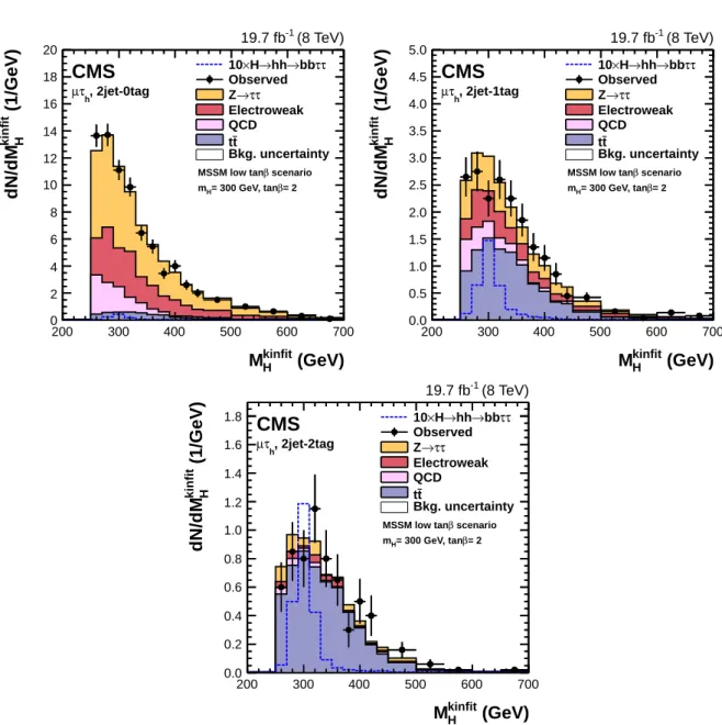
For the H→hh→bbττ process, the chosen distribution for signal extraction is the four-body mass. The decay products of the two h bosons need to fulfill stringent kinematic constraints, due to the small natural width of the h. These constraints can be used in a kinematic fit in order to improve the event reconstruction and to better separate signal events from background. The collinear approximation for the decay products of the τ leptons is assumed in the fit, since the τleptons are highly boosted as they originate from an object that is heavy when compared to their own mass. Furthermore, it is assumed that the reconstruction of the directions of all final state objects is accurate and the uncertainties can be neglected compared to the uncertainties on the energy reconstruction. In the decay of the two τ leptons, at least two neutrinos are involved and there is no precise measurement of the original τ lepton energies. For this reason, the τlepton energies are constrained from the balance of the fitted H boson transverse momentum and the reconstructed transversal recoil determined from ETmiss reconstruction algorithms, as described in Sec. 3. The reconstructed mass obtained with the kinematic fit is denoted by mkinfitH (see Appendix A for a detailed description).
The signal-to-background ratio is greatly improved by selecting events that are consistent with a mass of 125 GeV for both the dijet (mbb) mass and the ditau mass (mττ) reconstructed with
SVFIT. The mass windows of the selections are optimised to collect as much signal as possible
while rejecting a large part of the background. They correspond to 70 < mbb < 150 GeV and 90 < mττ < 150 GeV. The invariant mass distributions of the H boson in different final states
are shown in Figs. 3, 4 and 5.
For the A → Zh → ``ττ process, the A boson mass is reconstructed from the four-vector in-formation of the Z boson candidate and the four-vector inin-formation of the h boson candidate as obtained from SVFIT. The invariant mass distributions of the A boson in the different
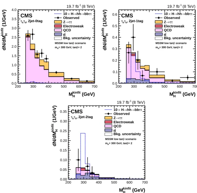
(GeV) kinfit H M 200 300 400 500 600 700 (1/GeV) kinfit H dN/dM 0 2 4 6 8 10 12 14 16 18 20 CMS (8 TeV) -1 19.7 fb , 2jet-0tag h τ µ scenario β MSSM low tan = 2 β = 300 GeV, tan H m τ τ bb → hh → H × 10 Observed τ τ → Z Electroweak QCD t t Bkg. uncertainty (GeV) kinfit H M 200 300 400 500 600 700 (1/GeV) kinfit H dN/dM 0.0 0.5 1.0 1.5 2.0 2.5 3.0 3.5 4.0 4.5 5.0 CMS (8 TeV) -1 19.7 fb , 2jet-1tag h τ µ scenario β MSSM low tan = 2 β = 300 GeV, tan H m τ τ bb → hh → H × 10 Observed τ τ → Z Electroweak QCD t t Bkg. uncertainty (GeV) kinfit H M 200 300 400 500 600 700 (1/GeV) kinfit H dN/dM 0.0 0.2 0.4 0.6 0.8 1.0 1.2 1.4 1.6 1.8 CMS (8 TeV) -1 19.7 fb , 2jet-2tag h τ µ scenario β MSSM low tan = 2 β = 300 GeV, tan H m τ τ bb → hh → H × 10 Observed τ τ → Z Electroweak QCD t t Bkg. uncertainty
Figure 3: Distributions of the reconstructed four-body mass with the kinematic fit after apply-ing mass selections on mττ and mbb in the µτh channel. The plots are shown for events in the 2jet–0tag (top left), 2jet–1tag (top right), and 2jet–2tag (bottom) categories. The expected signal scaled by a factor 10 is shown superimposed as an open dashed histogram for tan β = 2 and mH = 300 GeV in the low tan β scenario of the MSSM. Expected background contributions are shown for the values of nuisance parameters (systematic uncertainties) obtained after fitting the signal plus background hypothesis to the data.
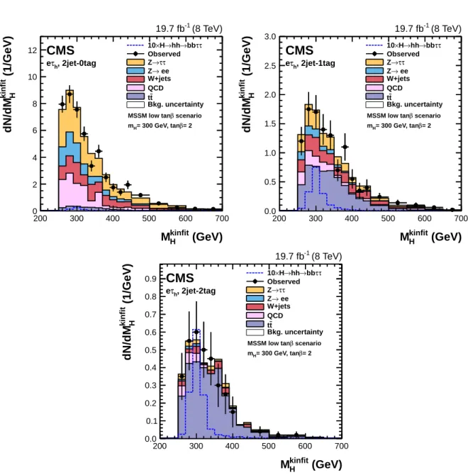
(GeV) kinfit H M 200 300 400 500 600 700 (1/GeV) kinfit H dN/dM 0 2 4 6 8 10 12 CMS (8 TeV) -1 19.7 fb , 2jet-0tag h τ e scenario β MSSM low tan = 2 β = 300 GeV, tan H m τ τ bb → hh → H × 10 Observed τ τ → Z ee → Z W+jets QCD t t Bkg. uncertainty (GeV) kinfit H M 200 300 400 500 600 700 (1/GeV) kinfit H dN/dM 0.0 0.5 1.0 1.5 2.0 2.5 3.0 CMS (8 TeV) -1 19.7 fb , 2jet-1tag h τ e scenario β MSSM low tan = 2 β = 300 GeV, tan H m τ τ bb → hh → H × 10 Observed τ τ → Z ee → Z W+jets QCD t t Bkg. uncertainty (GeV) kinfit H M 200 300 400 500 600 700 (1/GeV) kinfit H dN/dM 0.0 0.1 0.2 0.3 0.4 0.5 0.6 0.7 0.8 0.9 CMS (8 TeV) -1 19.7 fb , 2jet-2tag h τ e scenario β MSSM low tan = 2 β = 300 GeV, tan H m τ τ bb → hh → H × 10 Observed τ τ → Z ee → Z W+jets QCD t t Bkg. uncertainty
Figure 4: Distributions of the reconstructed four-body mass with the kinematic fit after apply-ing mass selections on mττ and mbb in the eτh channel. The plots are shown for events in the 2jet–0tag (top left), 2jet–1tag (top right), and 2jet–2tag (bottom) categories. The expected signal scaled by a factor 10 is shown superimposed as an open dashed histogram for tan β = 2 and mH = 300 GeV in the low tan β scenario of the MSSM. Expected background contributions are shown for the values of nuisance parameters (systematic uncertainties) obtained after fitting the signal plus background hypothesis to the data.
(GeV) kinfit H M 200 300 400 500 600 700 (1/GeV) kinfit H dN/dM 0.0 0.5 1.0 1.5 2.0 2.5 3.0 3.5 4.0 CMS (8 TeV) -1 19.7 fb , 2jet-0tag h τ h τ scenario β MSSM low tan = 2 β = 300 GeV, tan H m τ τ bb → hh → H × 10 Observed τ τ → Z Electroweak QCD t t Bkg. uncertainty (GeV) kinfit H M 200 300 400 500 600 700 (1/GeV) kinfit H dN/dM 0.0 0.1 0.2 0.3 0.4 0.5 0.6 CMS (8 TeV) -1 19.7 fb , 2jet-1tag h τ h τ scenario β MSSM low tan = 2 β = 300 GeV, tan H m τ τ bb → hh → H × 10 Observed τ τ → Z Electroweak QCD t t Bkg. uncertainty (GeV) kinfit H M 200 300 400 500 600 700 (1/GeV) kinfit H dN/dM 0.00 0.05 0.10 0.15 0.20 0.25 0.30 0.35 CMS (8 TeV) -1 19.7 fb , 2jet-2tag h τ h τ scenario β MSSM low tan = 2 β = 300 GeV, tan H m τ τ bb → hh → H × 10 Observed τ τ → Z Electroweak QCD t t Bkg. uncertainty
Figure 5: Distributions of the reconstructed four-body mass with the kinematic fit after apply-ing mass selections on mττ and mbbin the τhτhchannel. The plots are shown for events in the 2jet–0tag (top left), 2jet–1tag (top right), and 2jet–2tag (bottom) categories. The expected signal scaled by a factor 10 is shown superimposed as an open dashed histogram for tan β = 2 and mH = 300 GeV in the low tan β scenario of the MSSM. Expected background contributions are shown for the values of nuisance parameters (systematic uncertainties) obtained after fitting the signal plus background hypothesis to the data.
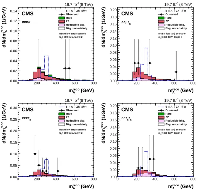
from reducible and irreducible backgrounds, while the``eµ final states are dominated by the irreducible ZZ production. The background in labelled as “rare” collects together the smaller contributions from the triboson processes as discussed in the previous section.
(GeV) reco A m 0 200 400 600 800 (1/GeV) reco A dN/dm 0.00 0.02 0.04 0.06 0.08 0.10 0.12 0.14 5 × A→ Zh→llττ Observed Rare ZZ Reducible bkg. Bkg. uncertainty (8 TeV) -1 19.7 fb
CMS
scenario β MSSM low tan = 2 β = 300 GeV, tan A m µ eee (GeV) reco A m 0 200 400 600 800 (1/GeV) reco A dN/dm 0.00 0.02 0.04 0.06 0.08 0.10 0.12 0.14 0.16 0.18 0.20 5 × A→ Zh→llττ Observed Rare ZZ Reducible bkg. Bkg. uncertainty (8 TeV) -1 19.7 fbCMS
scenario β MSSM low tan = 2 β = 300 GeV, tan A m h τ µ ee (GeV) reco A m 0 200 400 600 800 (1/GeV) reco A dN/dm 0.00 0.05 0.10 0.15 0.20 0.25 0.30 5 × A→ Zh→llττ Observed Rare ZZ Reducible bkg. Bkg. uncertainty (8 TeV) -1 19.7 fbCMS
scenario β MSSM low tan = 2 β = 300 GeV, tan A m h τ eee (GeV) reco A m 0 200 400 600 800 (1/GeV) reco A dN/dm 0.00 0.02 0.04 0.06 0.08 0.10 0.12 0.14 0.16 0.18 0.20 5 × A→ Zh→llττ Observed Rare ZZ Reducible bkg. Bkg. uncertainty (8 TeV) -1 19.7 fbCMS
scenario β MSSM low tan = 2 β = 300 GeV, tan A m h τ h τ eeFigure 6: Invariant mass distributions for different final states of the A → Zh process where Z decays to ee. The expected signal scaled by a factor 5 is shown superimposed as an open dashed histogram for tan β = 2 and mA = 300 GeV in the low tan β scenario of MSSM. Ex-pected background contributions are shown for the values of nuisance parameters (systematic uncertainties) obtained after fitting the signal plus background hypothesis to the data.
In neither search do the invariant mass spectra show any evidence of a signal. Model indepen-dent upper limits at 95% confidence level (CL) on the cross section times branching fraction are set using a binned maximum likelihood fit for the signal plus background and background– only hypotheses. The limits are determined using the CLsmethod [73, 74] and the procedure is described in Ref. [75, 76].
Systematic uncertainties are taken into account as nuisance parameters in the fit procedure: normalisation uncertainties affect the signal and background yields. Uncertainties on the τ
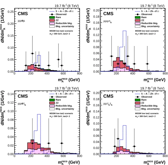
(GeV) reco A m 0 200 400 600 800 (1/GeV) reco A dN/dm 0.00 0.05 0.10 0.15 0.20 0.25 5 × A→ Zh→llττ Observed Rare ZZ Reducible bkg. Bkg. uncertainty (8 TeV) -1 19.7 fb
CMS
scenario β MSSM low tan = 2 β = 300 GeV, tan A m µ e µ µ (GeV) reco A m 0 200 400 600 800 (1/GeV) reco A dN/dm 0.00 0.02 0.04 0.06 0.08 0.10 0.12 0.14 0.16 0.18 0.20 5 × A→ Zh→llττ Observed Rare ZZ Reducible bkg. Bkg. uncertainty (8 TeV) -1 19.7 fbCMS
scenario β MSSM low tan = 2 β = 300 GeV, tan A m h τ µ µ µ (GeV) reco A m 0 200 400 600 800 (1/GeV) reco A dN/dm 0.00 0.02 0.04 0.06 0.08 0.10 0.12 0.14 5 × A→ Zh→llττ Observed Rare ZZ Reducible bkg. Bkg. uncertainty (8 TeV) -1 19.7 fbCMS
scenario β MSSM low tan = 2 β = 300 GeV, tan A m h τ e µ µ (GeV) reco A m 0 200 400 600 800 (1/GeV) reco A dN/dm 0.00 0.02 0.04 0.06 0.08 0.10 0.12 0.14 0.16 0.18 0.20 5 × A→ Zh→llττ Observed Rare ZZ Reducible bkg. Bkg. uncertainty (8 TeV) -1 19.7 fbCMS
scenario β MSSM low tan = 2 β = 300 GeV, tan A m h τ h τ µ µFigure 7: Invariant mass distributions for different final states of the A → Zh process where Z decays to µµ. The expected signal scaled by a factor 5 is shown superimposed as an open dashed histogram for tan β = 2 and mA = 300 GeV in the low tan β scenario of MSSM. Ex-pected background contributions are shown for the values of nuisance parameters (systematic uncertainties) obtained after fitting the signal plus background hypothesis to the data.
energy scale and jet energy scale are propagated as shape uncertainties.
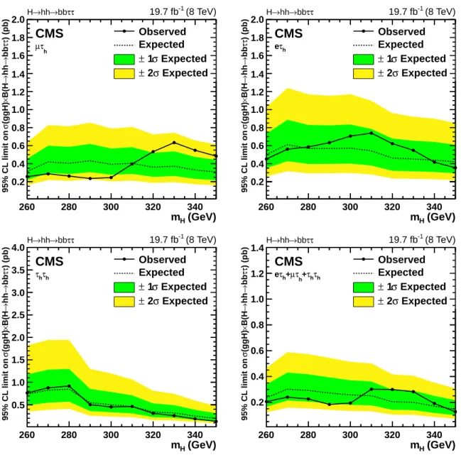
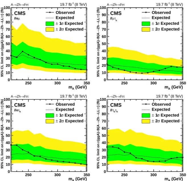
The model independent expected and observed cross section times branching fraction limits for the H →hh → bbττ process are shown in Fig. 8 and for the A → Zh → LLττ process in Figs. 9 and 10 where L=e, µ or τ in order to reflect the small Z→ττcontribution to the signal acceptance. (GeV) H m 260 280 300 320 340 ) (pb) ττ bb → hh → B(H × (ggH) σ 9 5 % C L l im it o n 0.2 0.4 0.6 0.8 1.0 1.2 1.4 1.6 1.8 2.0 Observed Expected Expected σ 1 ± Expected σ 2 ± CMS (8 TeV) -1 19.7 fb h τ µ τ τ bb → hh → H (GeV) H m 260 280 300 320 340 ) (pb) ττ bb → hh → B(H × (ggH) σ 9 5 % C L l im it o n 0.2 0.4 0.6 0.8 1.0 1.2 1.4 1.6 1.8 2.0 Observed Expected Expected σ 1 ± Expected σ 2 ± CMS (8 TeV) -1 19.7 fb h τ e τ τ bb → hh → H (GeV) H m 260 280 300 320 340 ) (pb) ττ bb → hh → B(H × (ggH) σ 9 5 % C L l im it o n 0.5 1.0 1.5 2.0 2.5 3.0 3.5 4.0 Observed Expected Expected σ 1 ± Expected σ 2 ± CMS (8 TeV) -1 19.7 fb h τ h τ τ τ bb → hh → H (GeV) H m 260 280 300 320 340 ) (pb) ττ bb → hh → B(H × (ggH) σ 9 5 % C L l im it o n 0.2 0.4 0.6 0.8 1.0 1.2 1.4 Observed Expected Expected σ 1 ± Expected σ 2 ± CMS (8 TeV) -1 19.7 fb h τ h τ + h τ µ + h τ e τ τ bb → hh → H
Figure 8: Upper limits at 95% CL on the H→hh→bbττ cross section times branching fraction for the µτh (top left), eτh(top right), τhτh(bottom left), and for final states combined (bottom right)
We interpret the observed limits on the cross section times branching fraction in the MSSM and 2HDM frameworks, discussed in Section 1.
In the MSSM we interpret them in the “low tanβ” scenario [27, 77] in which the value of MSUSY is increased until the mass of the lightest Higgs boson is consistent with 125 GeV over a range of low tan β and mAvalues. The exclusion region in the mA-tan β plane for the combination of the H → hh → bbττ and A → Zh → ``ττ analyses, in such a scenario, is shown in Fig. 11. The limit falls off rapidly as mAapproaches 350 GeV because decays of the A to two top quarks
(GeV) A m 250 300 350 ) (fb) ττ LL → Zh → B(A × (ggA) σ 9 5 % C L l im it o n 0 10 20 30 40 50 60 70 80 90 100 Observed Expected Expected σ 1 ± Expected σ 2 ± CMS (8 TeV) -1 19.7 fb µ e ll τ τ ll → Zh → A (GeV) A m 250 300 350 ) (fb) ττ LL → Zh → B(A × (ggA) σ 9 5 % C L l im it o n 0 10 20 30 40 50 60 70 80 90 100 Observed Expected Expected σ 1 ± Expected σ 2 ± CMS (8 TeV) -1 19.7 fb h τ µ ll τ τ ll → Zh → A (GeV) A m 250 300 350 ) (fb) ττ LL → Zh → B(A × (ggA) σ 9 5 % C L l im it o n 0 10 20 30 40 50 60 70 80 90 100 Observed Expected Expected σ 1 ± Expected σ 2 ± CMS (8 TeV) -1 19.7 fb h τ e ll τ τ ll → Zh → A (GeV) A m 250 300 350 ) (fb) ττ LL → Zh → B(A × (ggA) σ 9 5 % C L l im it o n 0 10 20 30 40 50 60 70 80 90 100 Observed Expected Expected σ 1 ± Expected σ 2 ± CMS (8 TeV) -1 19.7 fb h τ h τ ll τ τ ll → Zh → A
Figure 9: Upper limits at 95% CL on cross section times branching fraction on A→Zh→LLττ for``eµ (top left),``µτh(top right),``eτh(bottom left), and``τhτh(bottom right) final states.
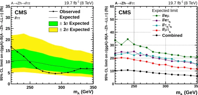
(GeV) A m 250 300 350 ) (fb) ττ LL → Zh → B(A × (ggA) σ 9 5 % C L l im it o n 0 5 10 15 20 25 30 35 Observed Expected Expected σ 1 ± Expected σ 2 ± CMS (8 TeV) -1 19.7 fb τ τ ll τ τ ll → Zh → A (GeV) A m 250 300 350 ) (fb) ττ LL → Zh → B(A × (ggA) σ 9 5 % C L l im it o n 0 10 20 30 40 50 60 CMS (8 TeV) -1 19.7 fb τ τ ll → Zh → A Expected limit µ e ll h τ e ll h τ h τ ll h τ µ ll Combined
Figure 10: Upper limits at 95% CL on cross section times branching fraction on A → Zh → LLττ for all``ττfinal states combined (left) and comparison of the different final states (right). are becoming kinematically allowed.
The interpretation of the observed limits in a Type II 2HDM is performed in the “physics basis”. The inputs to this interpretation are the physical Higgs boson masses (mh, mH, mA, mH±), the ratio of the vacuum expectation energies (tan β), the CP-even Higgs mixing angle (α) and m212 = m2A[tan β/(1+tan β2)]. For simplicity we assume that mH= mA= mH±.
The cross-sections and branching fractions in the 2HDM were calculated as described by the LHC Higgs Cross Section Working Group [77, 78]. The exclusion regions, calculated using the combination of the H→hh→bbττ and A→Zh→ ``ττanalyses, in the cos(β−α)vs. tan β plane for such a Type II 2HDM scenario with a heavy Higgs boson mass of 300 GeV are shown in Fig. 12. This can be compared to Fig. 5 in Ref. [41].
8
Summary
A search for a heavy scalar Higgs boson (H) decaying into a pair of SM-like Higgs bosons (hh) and a search for a heavy neutral pseudoscalar Higgs boson (A) decaying into a Z boson and a SM-like Higgs boson (h), have been performed using events recorded by the CMS experiment at the LHC. The dataset corresponds to an integrated luminosity of 19.7 fb−1, recorded at 8 TeV centre-of-mass energy in 2012. No evidence for a signal has been found and exclusion limits on the production cross section times branching fraction for the processes H → hh → bbττ and A → Zh → LLττ are presented. The results are also interpreted in the context of the MSSM and 2HDM models.
Acknowledgments
We congratulate our colleagues in the CERN accelerator departments for the excellent perfor-mance of the LHC and thank the technical and administrative staffs at CERN and at other CMS institutes for their contributions to the success of the CMS effort. In addition, we gratefully acknowledge the computing centres and personnel of the Worldwide LHC Computing Grid for delivering so effectively the computing infrastructure essential to our analyses. Finally, we
(GeV)
Am
250 300 350β
tan
1.0
1.5
2.0
2.5
3.0
3.5
4.0
95% CL Excluded: Observed ± 1σ Expected Expected ± 2σ Expected 3 GeV ± 125≠
h MSSM m scenario β MSSM low tanCMS
(8 TeV)
-119.7 fb
τ τ ll → Zh → + A τ τ bb → hh → HFigure 11: The 95% CL exclusion region in the mA-tan β plane for the low-tan β scenario as discussed in the introduction, combining the results of the H → hh → bbττ and the A → Zh → ``ττ analysis. The area highlighted in blue below the black curve marks the observed exclusion. The dashed curve and the grey bands show the expected exclusion limit with the relative uncertainty. The red area with the back-slash lines at the lower-left corner of the plot indicates the region excluded by the mass of the SM-like scalar boson being 125 GeV. The limit falls off rapidly as mAapproaches 350 GeV because decays of the A to two top quarks are becoming kinematically allowed.
)
α
-β
cos(
-1.0 -0.5 0.0 0.5 1.0β
tan
1
2
3
4
5
6
7
8
9
10
95% CL Excluded: Observed ± 1σ Expected Expected ± 2σ Expected = 300 GeV H = m A 2HDM type-II, mCMS
H→hh→bbττ+A→Zh→llττ 19.7 fb-1 (8 TeV)Figure 12: The 95% CL exclusion regions in the cos(β−α)vs. tan β plane of 2HDM Type II model for mA =mH =300 GeV, combining the results of the H→hh→bbττ and A→Zh→ ``ττ analysis. The areas highlighted in blue bounded by the black curves mark the observed exclusion. The dashed curves and the grey bands show the expected exclusion limit with the relative uncertainty.
CNRS/IN2P3 (France); BMBF, DFG, and HGF (Germany); GSRT (Greece); OTKA and NIH (Hungary); DAE and DST (India); IPM (Iran); SFI (Ireland); INFN (Italy); MSIP and NRF (Re-public of Korea); LAS (Lithuania); MOE and UM (Malaysia); CINVESTAV, CONACYT, SEP, and UASLP-FAI (Mexico); MBIE (New Zealand); PAEC (Pakistan); MSHE and NSC (Poland); FCT (Portugal); JINR (Dubna); MON, RosAtom, RAS and RFBR (Russia); MESTD (Serbia); SEIDI and CPAN (Spain); Swiss Funding Agencies (Switzerland); MST (Taipei); ThEPCenter, IPST, STAR and NSTDA (Thailand); TUBITAK and TAEK (Turkey); NASU and SFFR (Ukraine); STFC (United Kingdom); DOE and NSF (USA).
Individuals have received support from the Marie-Curie programme and the European Re-search Council and EPLANET (European Union); the Leventis Foundation; the A. P. Sloan Foundation; the Alexander von Humboldt Foundation; the Belgian Federal Science Policy Of-fice; the Fonds pour la Formation `a la Recherche dans l’Industrie et dans l’Agriculture (FRIA-Belgium); the Agentschap voor Innovatie door Wetenschap en Technologie (IWT-(FRIA-Belgium); the Ministry of Education, Youth and Sports (MEYS) of the Czech Republic; the Council of Science and Industrial Research, India; the HOMING PLUS programme of the Foundation for Polish Science, cofinanced from European Union, Regional Development Fund; the OPUS programme of the National Science Center (Poland); the Compagnia di San Paolo (Torino); the Consorzio per la Fisica (Trieste); MIUR project 20108T4XTM (Italy); the Thalis and Aristeia programmes cofinanced by EU-ESF and the Greek NSRF; the National Priorities Research Program by Qatar National Research Fund; the Rachadapisek Sompot Fund for Postdoctoral Fellowship, Chula-longkorn University (Thailand); and the Welch Foundation, contract C-1845.
References
[1] S. L. Glashow and S. Weinberg, “Natural conservation laws for neutral currents”, Phys. Rev. D 15 (1977) 1958, doi:10.1103/PhysRevD.15.1958.
[2] J. F. Gunion, H. E. Haber, G. Kane, and S. Dawson, “The Higgs Hunter’s Guide”. Addison-Wesley, 2000. [Frontiers in Physics, 80].
[3] G. C. Branco et al., “Theory and phenomenology of two-Higgs-doublet models”, Phys. Rept. 516 (2012) 1, doi:10.1016/j.physrep.2012.02.002, arXiv:1106.0034. [4] P. Fayet, “Supergauge invariant extension of the Higgs mechanism and a model for the
electron and its neutrino”, Nucl. Phys. B 90 (1975) 104, doi:10.1016/0550-3213(75)90636-7.
[5] P. Fayet, “Supersymmetry and weak, electromagnetic and strong interactions”, Phys. Lett. B 64 (1976) 159, doi:10.1016/0370-2693(76)90319-1.
[6] P. Fayet, “Spontaneously broken supersymmetric theories of weak, electromagnetic and strong interactions”, Phys. Lett. B 69 (1977) 489,
doi:10.1016/0370-2693(77)90852-8.
[7] S. Dimopoulos and H. Georgi, “Softly broken supersymmetry and SU(5)”, Nucl. Phys. B 193(1981) 150, doi:10.1016/0550-3213(81)90522-8.
[8] N. Sakai, “Naturalness in supersymmetric GUTS”, Z. Phys. C 11 (1981) 153, doi:10.1007/BF01573998.
[9] K. Inoue, A. Kakuto, H. Komatsu, and S. Takeshita, “Low-Energy Parameters and
Particle Masses in a Supersymmetric Grand Unified Model”, Prog. Theor. Phys. 67 (1982) 1889, doi:10.1143/PTP.67.1889.
[10] K. Inoue, A. Kakuto, H. Komatsu, and S. Takeshita, “Aspects of Grand Unified Models with Softly Broken Supersymmetry”, Prog. Theor. Phys. 68 (1982) 927,
doi:10.1143/PTP.68.927.
[11] K. Inoue, A. Kakuto, H. Komatsu, and S. Takeshita, “Renormalization of Supersymmetry Breaking Parameters Revisited”, Prog. Theor. Phys. 71 (1984) 413,
doi:10.1143/PTP.71.413.
[12] A. Djouadi, “The anatomy of electroweak symmetry breaking Tome II: The Higgs bosons in the Minimal Supersymmetric Model”, Phys. Rept. 459 (2008) 1,
doi:10.1016/j.physrep.2007.10.005, arXiv:hep-ph/0503173.
[13] Y. Okada, M. Yamaguchi, and T. Yanagida, “Upper Bound of the Lightest Higgs Boson Mass in the Minimal Supersymmetric Standard Model”, Prog. Theor. Phys. 85 (1991) 1, doi:10.1143/PTP/85.1.1.
[14] J. R. Ellis, G. Ridolfi, and F. Zwirner, “Radiative corrections to the masses of supersymmetric Higgs bosons”, Phys. Lett. B 257 (1991) 83,
doi:10.1016/0370-2693(91)90863-L.
[15] H. E. Haber and R. Hempfling, “Can the Mass of the Lightest Higgs Boson of the Minimal Supersymmetric Model be Larger than mZ?”, Phys. Rev. Lett. 66 (1991) 1815, doi:10.1103/PhysRevLett.66.1815.
¯tbH+interaction in the MSSM and charged Higgs phenomenology”, Nucl. Phys. B 577 (2000) 88, doi:10.1016/S0550-3213(00)00146-2, arXiv:hep-ph/9912516. [18] CMS Collaboration, “Search for neutral MSSM Higgs bosons decaying to a pair of tau
leptons in pp collisions”, JHEP 10 (2014) 160, doi:10.1007/JHEP10(2014)160, arXiv:1408.3316.
[19] CMS Collaboration, “Search for neutral MSSM Higgs bosons decaying into a pair of bottom quarks”, (2015). arXiv:1506.08329.
[20] ATLAS Collaboration, “Search for neutral Higgs bosons of the minimal supersymmetric standard model in pp collisions at√s = 8 TeV with the ATLAS detector”, JHEP 11 (2014) 056, doi:10.1007/JHEP11(2014)056, arXiv:1409.6064.
[21] M. S. Carena et al., “MSSM Higgs boson searches at the LHC: benchmark scenarios after the discovery of a Higgs-like particle”, Eur. Phys. J. C 73 (2013) 2552,
doi:10.1140/epjc/s10052-013-2552-1, arXiv:1302.7033.
[22] ATLAS and CMS Collaboration, “Combined Measurement of the Higgs Boson Mass in pp Collisions at√s=7 and 8 TeV with the ATLAS and CMS Experiments”, Phys. Rev. Lett. 114(2015) 191803, doi:10.1103/PhysRevLett.114.191803, arXiv:1503.07589. [23] A. Djouadi and J. Quevillon, “The MSSM Higgs sector at a high MSUSY: reopening the
low tanβ regime and heavy Higgs searches”, JHEP 10 (2013) 028, doi:10.1007/JHEP10(2013)028, arXiv:1304.1787.
[24] M. Carena et al., “Complementarity between nonstandard Higgs boson searches and precision Higgs boson measurements in the MSSM”, Phys. Rev. D 91 (2015) 035003, doi:10.1103/PhysRevD.91.035003, arXiv:1410.4969.
[25] A. Djouadi et al., “The post-Higgs MSSM scenario: habemus MSSM?”, Eur. Phys. J. C 73 (2013) 2650, doi:10.1140/epjc/s10052-013-2650-0, arXiv:1307.5205.
[26] A. Djouadi et al., “Fully covering the MSSM Higgs sector at the LHC”, (2015). arXiv:1502.05653.
[27] E. Bagnaschi et al., “Benchmark scenarios for low tan β in the MSSM”, Technical Report LHCHXSWG-2015-002, CERN, Geneva, Aug, 2015.
[28] A. Arbey, M. Battaglia, and F. Mahmoudi, “Supersymmetric heavy Higgs bosons at the LHC”, Phys. Rev. D 88 (2013) 015007, doi:10.1103/PhysRevD.88.015007,
arXiv:1303.7450.
[29] ATLAS Collaboration, “Observation of a new particle in the search for the Standard Model Higgs boson with the ATLAS detector at the LHC”, Phys. Lett. B 716 (2012) 1, doi:10.1016/j.physletb.2012.08.020, arXiv:1207.7214.
[30] CMS Collaboration, “Observation of a new boson at a mass of 125 GeV with the CMS experiment at the LHC”, Phys. Lett. B 716 (2012) 30,
[31] CMS Collaboration, “Observation of a new boson with mass near 125 GeV in pp collisions at√s = 7 and 8 TeV”, JHEP 06 (2013) 081,
doi:10.1007/JHEP06(2013)081, arXiv:1303.4571.
[32] D. M. Asner et al., “ILC Higgs White Paper”, (2013). arXiv:1310.0763.
[33] CMS Collaboration, “Evidence for the direct decay of the 125 GeV Higgs boson to
fermions”, Nature Phys. 10 (2014) 557, doi:10.1038/nphys3005, arXiv:1401.6527. [34] CMS Collaboration, “Evidence for the 125 GeV Higgs boson decaying to a pair of τ
leptons”, JHEP 05 (2014) 104, doi:10.1007/JHEP05(2014)104, arXiv:1401.5041. [35] ATLAS Collaboration, “Search For Higgs Boson Pair Production in the γγb¯b Final State
using pp Collision Data at√s=8 TeV from the ATLAS Detector”, Phys. Rev. Lett. 114 (2015) 081802, doi:10.1103/PhysRevLett.114.081802, arXiv:1406.5053. [36] ATLAS Collaboration, “Search for a CP-odd Higgs boson decaying to Zh in pp collisions
at√s=8 TeV with the ATLAS detector”, Phys. Lett. B 744 (2015) 163, doi:10.1016/j.physletb.2015.03.054, arXiv:1502.04478.
[37] ATLAS Collaboration, “Search for Higgs boson pair production in the b¯bb¯b final state from pp collisions at√s=8 TeV with the ATLAS detector”, Eur. Phys. J. C (2015), no. 75, 412, doi:10.1140/epjc/s10052-015-3628-x, arXiv:1506.00285.
[38] ATLAS Collaboration, “Searches for Higgs boson pair production in the
hh→bbττ, γγWW∗, γγbb, bbbb channels with the ATLAS detector”, Phys. Rev. D 92 (2015), no. 9, 092004, doi:10.1103/PhysRevD.92.092004, arXiv:1509.04670. [39] CMS Collaboration, “Searches for heavy Higgs bosons in two-Higgs-doublet models and
for t→ch decay using multilepton and diphoton final states in pp collisions at 8 TeV”, Phys. Rev. D 90 (2014) 112013, doi:10.1103/PhysRevD.90.112013,
arXiv:1410.2751.
[40] CMS Collaboration, “Search for resonant pair production of Higgs bosons decaying to two bottom quark-antiquark pairs in proton-proton collisions at 8 TeV”, (2015).
arXiv:1503.04114.
[41] CMS Collaboration, “Search for a pseudoscalar boson decaying into a Z boson and the 125 GeV Higgs boson in l+l−b¯b final states”, (2015). arXiv:1504.04710.
[42] CMS Collaboration, “The CMS experiment at the CERN LHC”, JINST 3 (2008) S08004, doi:10.1088/1748-0221/3/08/S08004.
[43] T. Sj ¨ostrand, S. Mrenna, and P. Z. Skands, “PYTHIA 6.4 physics and manual”, JHEP 05 (2006) 026, doi:10.1088/1126-6708/2006/05/026, arXiv:hep-ph/0603175. [44] J. Alwall et al., “MadGraph 5: going beyond”, JHEP 06 (2011) 128,
doi:10.1007/JHEP06(2011)128, arXiv:1106.0522.
[45] P. Nason, “A New method for combining NLO QCD with shower Monte Carlo algorithms”, JHEP 11 (2004) 040, doi:10.1088/1126-6708/2004/11/040, arXiv:hep-ph/0409146.
[46] S. Frixione, P. Nason, and C. Oleari, “Matching NLO QCD computations with parton shower simulations: the POWHEG method”, JHEP 11 (2007) 070,
[48] S. Alioli, P. Nason, C. Oleari, and E. Re, “A general framework for implementing NLO calculations in shower Monte Carlo programs: the POWHEG BOX”, JHEP 06 (2010) 043, doi:10.1007/JHEP06(2010)043, arXiv:1002.2581.
[49] CMS Collaboration, “Jet and underlying event properties as a function of
charged-particle multiplicity in proton-proton collisions at√s=7 TeV”, Eur. Phys. J. C 73(2013) 2674, doi:10.1140/epjc/s10052-013-2674-5, arXiv:1310.4554. [50] N. Davidson et al., “Universal interface of TAUOLA: Technical and physics
documentation”, Comput. Phys. Commun. 183 (2012) 821, doi:10.1016/j.cpc.2011.12.009, arXiv:1002.0543.
[51] GEANT4 Collaboration, “GEANT4 — a simulation toolkit”, Nucl. Instrum. Meth. A 506 (2003) 250, doi:10.1016/S0168-9002(03)01368-8.
[52] H.-L. Lai et al., “New parton distributions for collider physics”, Phys. Rev. D 82 (2010) 074024, doi:10.1103/PhysRevD.82.074024, arXiv:1007.2241.
[53] J. Pumplin et al., “New generation of parton distributions with uncertainties from global QCD analysis”, JHEP 07 (2002) 012, doi:10.1088/1126-6708/2002/07/012, arXiv:hep-ph/0201195.
[54] A. D. Martin, W. J. Stirling, R. S. Thorne, and G. Watt, “Parton distributions for the LHC”, Eur. Phys. J. C 63 (2009) 189, doi:10.1140/epjc/s10052-009-1072-5,
arXiv:0901.0002.
[55] M. Botje et al., “The PDF4LHC Working Group Interim Recommendations”, (2011). arXiv:1101.0538.
[56] CMS Collaboration, “Particle–Flow Event Reconstruction in CMS and Performance for Jets, Taus, and EmissT ”, CMS Physics Analysis Summary CMS-PAS-PFT-09-001, 2009. [57] CMS Collaboration, “Commissioning of the Particle-flow Event Reconstruction with the
first LHC collisions recorded in the CMS detector”, CMS Physics Analysis Summary CMS-PAS-PFT-10-001, 2010.
[58] CMS Collaboration, “Performance of CMS muon reconstruction in pp collision events at√ s =7 TeV”, JINST 7 (2012) P10002, doi:10.1088/1748-0221/7/10/P10002, arXiv:1206.4071.
[59] CMS Collaboration, “Performance of electron reconstruction and selection with the CMS detector in proton-proton collisions at sqrts=8 TeV”, JINST 10 (2015) P06005,
doi:10.1088/1748-0221/10/06/P06005, arXiv:1502.02701.
[60] CMS Collaboration, “The performance of the CMS muon detector in proton-proton collisions at sqrt(s) = 7 TeV at the LHC”, JINST 8 (2013) P11002,
[61] CMS Collaboration, “Measurements of inclusive W and Z cross sections in pp collisions at√s=7 TeV”, JHEP 01 (2011) 080, doi:10.1007/JHEP01(2011)080,
arXiv:1012.2466.
[62] M. Cacciari, G. P. Salam, and G. Soyez, “FastJet user manual”, Eur. Phys. J. C 72 (2012) 1896, doi:10.1140/epjc/s10052-012-1896-2, arXiv:1111.6097.
[63] M. Cacciari and G. P. Salam, “Dispelling the N3myth for the ktjet-finder”, Phys. Lett. B 641(2006) 57, doi:10.1016/j.physletb.2006.08.037, arXiv:hep-ph/0512210. [64] M. Cacciari and G. P. Salam, “Pileup subtraction using jet areas”, Phys. Lett. B 659 (2008)
119, doi:10.1016/j.physletb.2007.09.077, arXiv:0707.1378.
[65] CMS Collaboration, “Pileup Jet Identification”, CMS Physics Analysis Summary CMS-PAS-JME-13-005, 2013.
[66] CMS Collaboration, “Performance of the CMS missing transverse momentum reconstruction in pp data at√s = 8 TeV”, JINST 10 (2015) P02006,
doi:10.1088/1748-0221/10/02/P02006, arXiv:1411.0511.
[67] CMS Collaboration, “Identification of b-quark jets with the CMS experiment”, JINST 8 (2013) P04013, doi:10.1088/1748-0221/8/04/P04013, arXiv:1211.4462. [68] CMS Collaboration, “Reconstruction and identification of lepton decays to hadrons and
at CMS”, JINST 11 (2016), no. 01, P01019, doi:10.1088/1748-0221/11/01/P01019, arXiv:1510.07488.
[69] CMS Collaboration, “Measurement of the inclusive Z cross section via decays to tau pairs in pp collisions at√s=7 TeV”, JHEP 08 (2011) 117,
doi:10.1007/JHEP08(2011)117, arXiv:1104.1617.
[70] CMS Collaboration, “CMS Luminosity Based on Pixel Cluster Counting — Summer 2013 Update”, CMS Physics Analysis Summary CMS-PAS-LUM-13-001, 2013.
[71] CMS Collaboration, “Determination of Jet Energy Calibration and Transverse Momentum Resolution in CMS”, JINST 6 (2011) P11002,
doi:10.1088/1748-0221/6/11/P11002, arXiv:1107.4277.
[72] L. Bianchini, J. Conway, E. K. Friis, and C. Veelken, “Reconstruction of the Higgs mass in H→ττEvents by Dynamical Likelihood techniques”, J. Phys. Conf. Ser. 513 (2014) 022035, doi:10.1088/1742-6596/513/2/022035.
[73] T. Junk, “Confidence level computation for combining searches with small statistics”, Nucl. Instrum. Meth. A 434 (1999) 435, doi:10.1016/S0168-9002(99)00498-2, arXiv:hep-ex/9902006.
[74] A. L. Read, “Presentation of search results: The CLstechnique”, J. Phys. G 28 (2002) 2693, doi:10.1088/0954-3899/28/10/313.
[75] ATLAS and CMS, LHC Higgs Combination Group, “Procedure for the LHC Higgs boson search combination in Summer 2011”, Technical Report ATL-PHYS-PUB 2011-11, CMS NOTE 2011/005, CERN, 2011.
[77] R. V. Harlander, S. Liebler, and H. Mantler, “SusHi: A program for the calculation of Higgs production in gluon fusion and bottom-quark annihilation in the Standard Model and the MSSM”, Comput. Phys. Commun. 184 (2013) 1605,
doi:10.1016/j.cpc.2013.02.006, arXiv:1212.3249.
[78] R. Harlander et al., “Interim recommendations for the evaluation of Higgs production cross sections and branching ratios at the LHC in the Two-Higgs-Doublet Model”, (2013). arXiv:1312.5571.
A
Kinematic Fit
In the analysed event topology H → hh → bbττ, the collinear approximation for the decay products of the τ leptons is assumed. This is well motivated, since the τ leptons are highly boosted as they originate from a relatively heavy object compared to their own mass, mh/mτ =
70. Further, it is assumed that the reconstruction of the directions of all final state objects ηiand φiwith i∈ {b1, b2, τ1vis, τ2vis}is accurate and the uncertainties can be neglected compared to the uncertainties on the energy reconstruction.
Both, the pair of b jets and the pair of τ leptons need to fulfil an invariant mass constraint m(τ1, τ2) =m(b1, b2) =mh =125 GeV. (2) These two hard constraints reduce the number of fit parameters to two, chosen to be Eb1 and
Eτ1.
For the two measured b jet energies, the χ2terms can be formulated as
χ2b1,2 = Efit b1,2−E meas b1,2 σb1,2 !2 , (3) where Ebfit
1,2are the fitted and E
meas
b1,2 are the reconstructed b jet energy, and σb1,2 describe the b jet
energy resolution.
In the decay of the two τ leptons at least two neutrinos are involved. Thus there exists no good measurement of the original τ lepton energies, but only lower energy limits. For this reason, the τ lepton energies are constrained from the balance of the fitted heavy Higgs boson transverse momentum ~pfitT,H = ~pfitT,b 1+ ~p fit T,b2 + ~p fit T,τ1+ ~p fit T,τ2 (4)
and the reconstructed transversal recoil
~pmeasT,recoil = −~pmeasT,miss− ~pT,bmeas1 − ~pmeasT,b2 − ~pmeasT,τvis
1
− ~pmeasT,τvis 2
= −~pmeasT,H . (5)
Herein,~pmeasT,miss denotes the reconstructed missing momentum in the transverse plane, which has been determined from Emiss
T reconstruction algorithms, as described in Sec. 3. Any nonzero residual vector~pres
T,recoil = ~pfitT,H+ ~pmeasT,recoil contributes to a χ2term as follows
χrecoil2 = ~pres,TT,recoil·Vrecoil−1 · ~presT,recoil, (6)
where Vrecoildenotes the covariance matrix of the reconstructed recoil vector. The overall χ2function finally reads,
χ2=χ2b1+χ2b2+χ2recoil. (7)
After minimisation of this function by varying Eb1 and Eτ1, a very accurate reconstruction of