Identification of heavy-flavour jets with the CMS detector in pp collisions at 13 TeV

(1)

EUROPEAN ORGANIZATION FOR NUCLEAR RESEARCH (CERN)

CERN-EP-2017-326 2018/05/10

CMS-BTV-16-002

Identification of heavy-flavour jets with the CMS detector

in pp collisions at 13 TeV

The CMS Collaboration

∗

Abstract

Many measurements and searches for physics beyond the standard model at the LHC rely on the efficient identification of heavy-flavour jets, i.e. jets originating from bot-tom or charm quarks. In this paper, the discriminating variables and the algorithms used for heavy-flavour jet identification during the first years of operation of the CMS experiment in proton-proton collisions at a centre-of-mass energy of 13 TeV, are pre-sented. Heavy-flavour jet identification algorithms have been improved compared to those used previously at centre-of-mass energies of 7 and 8 TeV. For jets with trans-verse momenta in the range expected in simulated tt events, these new developments result in an efficiency of 68% for the correct identification of a b jet for a probability of 1% of misidentifying a light-flavour jet. The improvement in relative efficiency at this misidentification probability is about 15%, compared to previous CMS algorithms. In addition, for the first time algorithms have been developed to identify jets containing two b hadrons in Lorentz-boosted event topologies, as well as to tag c jets. The large data sample recorded in 2016 at a centre-of-mass energy of 13 TeV has also allowed the development of new methods to measure the efficiency and misidentification proba-bility of heavy-flavour jet identification algorithms. The b jet identification efficiency is measured with a precision of a few per cent at moderate jet transverse momenta (between 30 and 300 GeV) and about 5% at the highest jet transverse momenta (be-tween 500 and 1000 GeV).

Published in the Journal of Instrumentation as doi:10.1088/1748-0221/13/05/P05011.

c

2018 CERN for the benefit of the CMS Collaboration. CC-BY-4.0 license

∗_{See Appendix B for the list of collaboration members}

(2)

(3)

Contents 1

1 Introduction

The success of the physics programme of the CMS experiment at the CERN LHC requires the particles created in the LHC collisions to be reconstructed and identified as accurately as possi-ble. With the exception of the top quark, quarks and gluons produced in pp collisions develop a parton shower and eventually hadronize giving rise to jets of collimated particles observed in the CMS detector. Heavy-flavour jet identification techniques exploit the properties of the hadrons in the jet to discriminate between jets originating from b or c quarks (heavy-flavour jets) and those originating from light-flavour quarks or gluons (light-flavour jets). The CMS Collaboration presented in Ref. [1] a set of b jet identification techniques used in physics anal-yses performed on LHC Run 1 pp collision data, collected in 2011 and 2012 at centre-of-mass energies of 7 and 8 TeV. This paper presents a comprehensive summary of the newly devel-oped and optimized techniques compared to our previous results. In particular, the larger

(4)

recorded data set of pp collisions at a centre-of-mass energy of 13 TeV during Run 2 of the LHC in 2016, allows the study of rarer high-momentum topologies in which daughter jets from a Lorentz-boosted parent particle merge into a single jet. Examples of such topologies include the identification of boosted Higgs bosons decaying to two b quarks, and of b jets from boosted top quarks. The identification of c jets is also of significant interest, e.g. for the study of Higgs boson decays to a pair of c quarks, and for top squark searches in the c quark plus neutralino final-state topology.

The paper is organized as follows. A brief summary of particle and jet reconstruction in the CMS detector is given in Section 2. Details about the simulated proton-proton collision sam-ples and the data-taking conditions are given in Section 3. The properties of heavy-flavour jets and the variables used to discriminate between these and other jets are discussed in Section 4, while the algorithms are presented in Sections 5 and 6. For some physics processes, it is im-portant to identify b jets at the trigger level. This topic is discussed in Section 7. The large recorded number of proton-proton (pp) collisions permits the exploration of new methods to measure the efficiency of the heavy-flavour jet identification algorithms using data. These new methods, as well as the techniques used during the Run 1, are summarized in Sections 8 and 9 for efficiency measurements in nonboosted and boosted event topologies, respectively.

2 The CMS detector

The central feature of the CMS apparatus is a superconducting solenoid of 6 m internal diame-ter and a magnetic field of 3.8 T. Within the solenoid volume are a silicon pixel and strip tracker, a lead tungstate crystal electromagnetic calorimeter (ECAL), and a brass and scintillator hadron calorimeter (HCAL), each composed of a barrel and two endcap sections, together providing

coverage in pseudorapidity (η) up to |η| = 3.0. Forward calorimeters extend the coverage

to |η| = 5.2. Muons are detected in the pseudorapidity range|η| < 2.4 using gas-ionization

chambers embedded in the steel flux-return yoke outside the solenoid.

The silicon tracker measures charged particles within the range|η| < 2.5. During the first two

years of Run 2 operation at a centre-of-mass energy of 13 TeV, the silicon tracker setup did not change compared to the Run 1 of the LHC. The trajectories of charged particles are recon-structed from the hits in the silicon tracking system using an iterative procedure with a Kalman

filter. The tracking efficiency is typically over 98% for tracks with a transverse momentum (pT)

above 1 GeV. For nonisolated particles with 1 < pT < 10 GeV and |η| < 1.4, the track

reso-lutions are typically 1.5% in pT and 25–90 (45–150) µm in the transverse (longitudinal) impact

parameter (IP) [2]. The pp interaction vertices are reconstructed by clustering tracks on the basis of their z coordinates at their points of closest approach to the centre of the beam spot using a deterministic annealing algorithm [3]. The position of each vertex is estimated with an adaptive vertex fit [4]. The resolution on the position is around 20 µm in the transverse plane and around 30 µm along the beam axis for primary vertices reconstructed using at least 50 tracks [2].

The global event reconstruction, also called particle-flow (PF) event reconstruction [5], consists of reconstructing and identifying each individual particle with an optimized combination of all subdetector information. In this process, the identification of the particle type (photon, elec-tron, muon, charged hadron, neutral hadron) plays an important role in the determination of the particle direction and energy. Photons, e.g. coming from neutral pion decays or from elec-tron bremsstrahlung, are identified as ECAL energy clusters not linked to the extrapolation of any charged-particle trajectory to the ECAL. Electrons, e.g. coming from photon conversions in the tracker material or from heavy-flavour hadron semileptonic decays, are identified as

(5)

3

combinations of charged-particle tracks reconstructed in the tracker and multiple ECAL en-ergy clusters corresponding to both the passage of the electron through the ECAL plus any associated bremsstrahlung photons. Muons, e.g. from the semileptonic decay of heavy-flavour hadrons, are identified as tracks reconstructed in the tracker combined with matching hits or tracks in the muon system, and matching energy deposits in the calorimeters. Charged hadrons are identified as charged particles not identified as electrons or muons. Finally, neutral hadrons are identified as HCAL energy clusters not matching any charged-particle track, or as ECAL and HCAL energy excesses with respect to the expected charged-hadron energy deposit. For each event, particles originating from the same interaction vertex are clustered into jets with

the infrared and collinear safe anti-kTalgorithm [6, 7], using a distance parameter R=0.4 (AK4

jets). Compared to the R=0.5 jets that were used in Run 1 physics analyses, jets reconstructed

with R = 0.4 are found to still contain most of the particles from the hadronization process,

while at the same time being less sensitive to particles from additional pp interactions (known as pileup) appearing in the same or adjacent bunch crossings. For studies involving boosted

topologies, jets are clustered with a larger distance parameter R = 0.8 (AK8 jets). The jet

momentum is determined as the vectorial sum of all particle momenta in the jet. Jet energy corrections are derived from the simulation and are confirmed with in situ measurements using

the energy balance in dijet, multijet, photon + jet, and leptonically decaying Z+jets events [8].

The jet energy resolution amounts typically to 15% at 10 GeV, 8% at 100 GeV, and 4% at 1 TeV [8].

For the studies presented here, jets are required to lie within the tracker acceptance (|η| <2.4)

and have pT > 20 GeV. The missing transverse momentum vector is defined as the projection

of the negative vector sum of the momenta of all reconstructed particles in an event on the

plane perpendicular to the beams. Its magnitude is referred to as pmiss_T .

The reconstructed vertex with the largest value of summed physics-object p2_T is taken to be

the primary pp interaction vertex (PV). The physics objects are the jets, clustered using the jet finding algorithm with the tracks assigned to the vertex as inputs, and the associated missing

transverse momentum, taken as the negative vector sum of the pTof those jets.

The energy of electrons is determined from a combination of the track momentum at the main interaction vertex, the corresponding ECAL cluster energies, and the energies of all brems-strahlung photons associated with the track. The momentum resolution for electrons with

pT ≈ 45 GeV from Z → ee decays ranges from 1.7% for nonshowering electrons, i.e. not

pro-ducing additional photons and electrons, in the barrel region (|η| <1.48), to 4.5% for showering

electrons in the endcaps (1.48 < |η| <3.0) [9]. Muons with 20 < pT <100 GeV have a relative

pTresolution of 1.3–2.0% in the barrel and less than 6% in the endcaps. The pTresolution in the

barrel is better than 10% for muons with pT up to 1 TeV [10]. The energy of charged hadrons

is determined from a combination of the track momentum and the corresponding ECAL and HCAL energy deposits, corrected for zero-suppression effects and for the response function of the calorimeters to hadronic showers. Finally, the energy of neutral hadrons is obtained from the corresponding corrected ECAL and HCAL energy deposits.

Events of interest are selected using a two-tiered trigger system [11]. The level-1 trigger (L1), composed of custom hardware processors, uses information from the calorimeters and muon detectors to select events at a rate of around 100 kHz. The second level, known as the high-level trigger (HLT), consists of a farm of processors running a version of the full event reconstruction software optimized for fast processing, and reduces the event rate to less than 1 kHz before data storage.

A more detailed description of the CMS detector, together with a definition of the coordinate system used and the relevant kinematic variables, can be found in Ref. [12].

(6)

3 Data and simulated samples

The results presented in this paper are based on the pp collision data set recorded at a centre-of-mass energy of 13 TeV by the CMS detector in 2016, corresponding to an integrated

lumi-nosity of 35.9 fb−1. Various event generators are used to model the relevant physics processes.

The interactions between particles and the material of the CMS detector are simulated using GEANT 4 [13–15]. The data and simulated samples are used to determine the heavy-flavour jet identification efficiency in various event topologies. When measuring the heavy-flavour jet identification efficiency or when comparing the data to the simulation, the number of simulated events is large enough to neglect the statistical uncertainty in the simulation unless mentioned otherwise.

The pair production of top quarks and electroweak single top quark production is performed

with thePOWHEG2.0 generator at next-to-leading order (NLO) accuracy [16–21]. The value of

the top quark mass used for the generation of the simulated samples is 172.5 GeV. The

sys-tematic uncertainty related to the value of the top quark mass mt is evaluated by varying it

by ±1 GeV. Alternative samples are used to assess parton shower uncertainties, as well as

factorization and normalization scale uncertainties at the matrix element and parton shower levels. Diboson WW, WZ, and ZZ events, referred to collectively as “VV” events, are

gener-ated at NLO accuracy with the MADGRAPH5 aMC@NLO2.2.2 generator [22], including

MAD-SPIN [23] and the FxFx merging scheme [24] between jets from matrix element calculations

and the parton shower description, or with the POWHEG 2.0 generator [25, 26]. The Z+jets

and W+jets events are generated with MADGRAPH5 aMC@NLO2.2.2 at leading order (LO),

using the MLM matching scheme [27]. Samples of events with a Kaluza–Klein graviton [28]

decaying to two Higgs bosons are also simulated with MADGRAPH5 aMC@NLO2.2.2 at LO for

graviton masses ranging between 1 and 3.5 TeV. Background events comprised uniquely of jets

produced through the strong interaction (multijet events) are generated withPYTHIA8.205 [29]

in different ˆpT bins, where ˆpT is defined as the average pT of the final-state partons.

Muon-enriched multijet samples are produced by forcing the decay of charged pions and kaons into

muons and by requiring a generated muon with pT >5 GeV.

PYTHIA8.205 is also used for the parton showering and hadronization of all the simulated sam-ples with the CMS underlying event tunes CUETP8M1 [30] using the NNPDF 2.3 [31] parton distribution functions. In the case of top quark pair production a modification of this tune is used, CUETP8M2T4 [32] using the NNPDF 3.0 [33] parton distribution functions.

Pileup interactions are modelled by overlaying the simulated events with additional

mini-mum bias collisions generated withPYTHIA8.205. These additional simulated events are then

reweighted to match the observed number of pileup interactions or the primary vertex multi-plicity in data.

4 Heavy-flavour jet discriminating variables

4.1 Properties of heavy-flavour jets

Algorithms for heavy-flavour jet identification use variables connected to the properties of heavy-flavour hadrons present in jets resulting from the radiation and hadronization of b or c quarks. For instance, the lifetime of hadrons containing b quarks is of the order of 1.5 ps, while the lifetime of c hadrons is 1 ps or less. This leads to typical displacements of a few mm to one cm for b hadrons, depending on their momentum, thus giving rise to displaced tracks from which a secondary vertex (SV) may be reconstructed, as illustrated in Fig. 1. The displacement

(7)

4.1 Properties of heavy-flavour jets 5 jet jet heavy-flavour jet PV SV displaced tracks IP charged lepton

Figure 1: Illustration of a heavy-flavour jet with a secondary vertex (SV) from the decay of a b or c hadron resulting in charged-particle tracks (including possibly a soft lepton) that are displaced with respect to the primary interaction vertex (PV), and hence with a large impact parameter (IP) value.

of tracks with respect to the primary vertex is characterized by their impact parameter, which is defined as the distance between the primary vertex and the tracks at their points of closest ap-proach. The vector pointing from the primary vertex to the point of closest approach is referred to as the impact parameter vector. The impact parameter value can be defined in three spatial dimensions (3D) or in the plane transverse to the beam line (2D). The longitudinal impact pa-rameter is defined in one dimension, along the beam line. The impact papa-rameter is defined to be positive or negative, with a positive sign indicating that the track is produced “upstream”. This means that the angle between the impact parameter vector and the jet axis is smaller than

π/2, where the jet axis is defined by the primary vertex and the direction of the jet momentum.

In addition, b and c quarks have a larger mass and harder fragmentation compared to the light quarks and massless gluons. As a result, the decay products of the heavy-flavour hadron have,

on average, a larger pTrelative to the jet axis than the other jet constituents. In approximately

20% (10%) of the cases, a muon or electron is present in the decay chain of a heavy b (c) hadron. Hence, apart from the properties of the reconstructed secondary vertex or displaced tracks, the presence of charged leptons is also exploited for heavy-flavour jet identification techniques and for measuring their performance in data.

In order to design and optimize heavy-flavour identification techniques, a reliable method is required for assigning a flavour to jets in simulated events. The jet flavour is determined by clustering not only the reconstructed final-state particles into jets, but also the generated b and c hadrons that do not have b and c hadrons as daughters respectively. To prevent these gen-erated hadrons from affecting the reconstructed jet momentum, the modulus of the hadron four-momentum is set to a small number, retaining only the directional information. This pro-cedure is known as ghost association [34]. Jets containing at least one b hadron are defined as b jets; the ones containing at least one c hadron and no b hadron are defined as c jets. The remaining jets are considered to be light-flavour (or “udsg”) jets. Since pileup interactions are not included during the hard-scattering event generation, jets from pileup interactions (“pileup jets”) in the simulation are tentatively identified as jets without a matched generated jet. The generated jets are reconstructed with the jet clustering algorithm mentioned in Section 2 ap-plied to the generated final-state particles (excluding neutrinos). The matching between the

reconstructed PF jets and the generated jets with pT > 8 GeV is performed by requiring the

angular distance between them to be∆R = p

(∆η)2_{+ (}_∆φ₎2 _< _{0.25. Using this flavour}

def-inition, jets arising from gluon splitting to bb are considered as b jets. In Sections 6, 8 and 9,

(8)

hadron daughters should be clustered in the jet. The studies presented in Sections 4 and 5 are

based on simulated events. For these studies, jets are removed if they are closer than∆R=0.4

to a generated charged lepton from a direct V boson decay. In addition, electrons or muons originating from gauge boson decays that are reconstructed as jets are removed if they carry

more than 60% of the jet pT, i.e. p`T/p

jet

T <0.6 is required, where p`T(p

jet

T ) is the pT of the lepton

(jet). No additional identification or isolation requirements are applied for muons or electrons.

4.2 Track selection and variables

The properties of the tracks clustered within the jet represent the basic inputs of all heavy-flavour jet identification (tagging) algorithms. Input variables for the tagging algorithms are constructed from the tracks after applying appropriate selection criteria. In particular, to ensure

a good momentum and impact parameter resolution, tracks are required to have pT > 1 GeV,

a χ2_{value of the trajectory fit normalized to the number of degrees of freedom below 5, and}

at least one hit in the pixel layers of the tracker detector. The last of these requirements is less stringent than the requirement used for b jet identification in Run 1, where at least eight hits were required in the pixel and strip tracker combined, of which at least two were pixel detector hits. The requirement on the number of hits was relaxed to cope with saturation effects that were observed at high occupancy in the readout electronics of the strip tracker during the first part of the 2016 data taking, leading to a reduced tracking and b tagging performance. The issues with the readout electronics have been fully resolved, with no side effects on the track-ing performance, but the relaxed requirement on the number of hits was kept since there was no impact on the final b tagging performance. Apart from the requirements on the quality of

the tracks, the presence of tracks from long-lived K0_S or Λ hadrons as well as from material

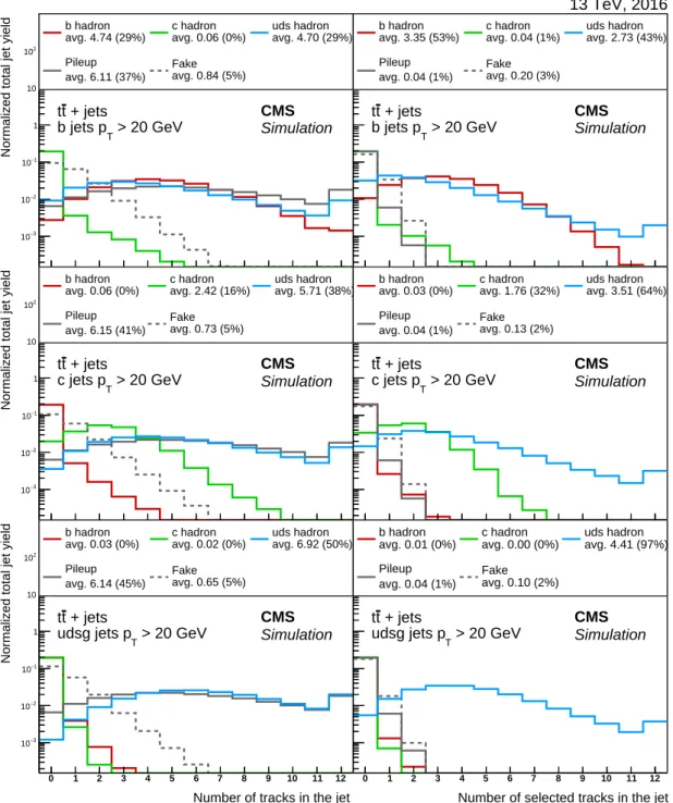
interactions is reduced by requiring the track decay length, defined as the distance from the primary vertex to the point of closest approach between the track and the jet axis, to be less than 5 cm. The contribution from tracks originating from pileup vertices is reduced with the following set of requirements: the absolute value of the transverse (longitudinal) impact pa-rameter of the track is required to be smaller than 0.2 (17) cm and the distance between the track and the jet axis at their point of closest approach is required to be less than 0.07 cm. Fig-ure 2 presents typical distributions of the latter variable for jets in tt events after applying the rest of the track selection requirements, showing the origin of each track separately. The origin of a track is labelled with “b hadron” if the track corresponds to a particle originating from a b hadron decay. A track corresponding to a particle from the decay of a c hadron that itself originates from the decay of a b hadron is also labelled as “b hadron”. The category with the “c hadron” label contains only tracks corresponding to a particle from the decay of a c hadron without a b hadron ancestor. The label “uds hadron” indicates tracks corresponding to parti-cles without heavy-flavour hadron ancestors. The label “pileup” refers to tracks from charged particles originating from a different primary vertex. A category with mismeasured tracks is defined containing tracks that are more likely to have been misreconstructed, e.g. by wrongly combining hits created by different particles. A track belongs to this category if the number of hits from the simulated charged particle closest to the track over the number of hits associated with the track, is less than 75%. This category is labelled as “fake”. In Fig. 3, the impact of the track selection requirements on the number of tracks in a given category is shown for various jet flavours in tt events. The track selection requirements clearly enhance the fraction of tracks originating from heavy-flavour hadron decays in bottom and charm jets. The track selection requirements reduce the number of tracks in the fake and pileup categories to a few per cent

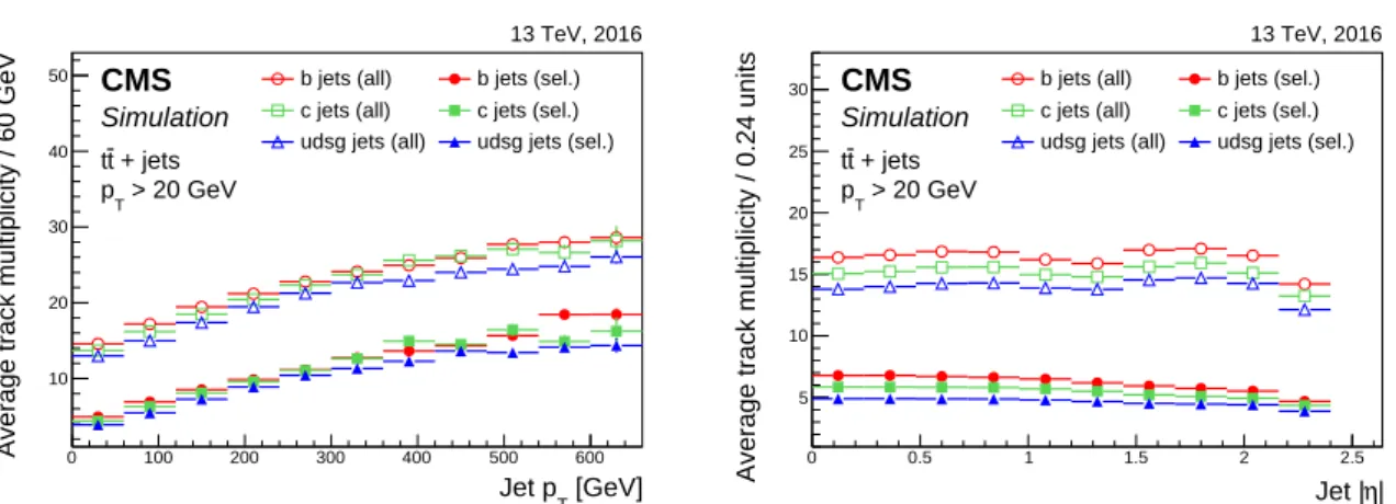
for all jet flavours. Figure 4 shows the track multiplicity dependence on the jet pT and|η|for

various jet flavours in tt events before and after applying the track selection requirements. For b jets, the average track multiplicity is higher than for light-flavour jets, before and after

(9)

apply-4.3 Secondary vertex reconstruction and variables 7

Distance between track and jet axis [cm]

0 0.1 0.2 0.3 0.4 0.5 Tracks / 0.01 cm 4 − 10 3 − 10 2 − 10 1 − 10 1 10

b hadron c hadron uds hadron

Pileup Fake + jets t t > 20 GeV T b jets p 13 TeV, 2016 CMS Simulation

Distance between track and jet axis [cm]

0 0.1 0.2 0.3 0.4 0.5 Tracks / 0.01 cm 4 − 10 3 − 10 2 − 10 1 − 10 1 10

b hadron c hadron uds hadron

Pileup Fake + jets t t > 20 GeV T udsg jets p 13 TeV, 2016 CMS Simulation

Figure 2: Distribution of the distance between a track and the jet axis at their point of closest approach for tracks associated with b (left) and light-flavour (right) jets in tt events. This dis-tance is required to be smaller than 0.07 cm, as indicated by the arrow. The tracks are divided into categories according to their origin as defined in the text. The distributions are normalized such that their sum has unit area. The last bin includes the overflow entries.

ing the track selection requirements, and the ratio of the average track multiplicity for b jets to other jet flavours is roughly constant. The average track multiplicity increases with increasing

jet pTfor all jet flavours. Before the track selection, the average track multiplicity is almost

con-stant with respect to the jet|η|. The small variations seen are due to the tracker geometry that

has an impact on the track reconstruction efficiency. In addition, since the η of the jet is defined as the η of the jet axis, some of the charged particles in the jet are outside the tracker acceptance

for high jet|η|values, resulting in a lower track multiplicity in the highest bin. When the track

selection requirements are applied, the average track multiplicity decreases with respect to the

jet|η|, because of the relatively larger impact of the track selection requirements near the edge

of the acceptance window for the tracker.

The aforementioned track selection requirements are always applied when reconstructing the variables used in the tagging algorithms. An exception is given by the variables relying on the inclusive vertex finding algorithm, as discussed in Section 4.3. Figure 5 shows the distribution of the 3D impact parameter and its significance for the different jet flavours. The impact pa-rameter significance is defined as the impact papa-rameter value divided by its uncertainty, IP/σ. In addition, the lower panels in Fig. 5 also show the distribution of the 2D impact parameter significance for the track with the highest and second-highest 2D impact parameter significance for different jet flavours. From Fig. 5 it is clear that tracks in heavy-flavour jets have larger im-pact parameter and imim-pact parameter significance compared to tracks in light-flavour jets. The lower left panel in Fig. 5 shows that tracks with a large impact parameter significance are also present in light-flavour jets. These originate from the decays of relatively long-lived hadrons,

for example K0_S or Λ, or from heavy-flavour hadrons where the tracks have been incorrectly

clustered into a light-flavour jet. For the track with the second-highest impact parameter sig-nificance in light-flavour jets, the distribution is much more symmetric as expected for hadrons with a short lifetime.

4.3 Secondary vertex reconstruction and variables

If the secondary vertex from the decay of a heavy-flavour hadron is reconstructed, powerful discriminating variables can be derived from it. An example is the (corrected) secondary ver-tex mass, which is directly related to the mass of the heavy-flavour hadron. The corrected

(10)

sec-13 TeV, 2016

Number of tracks in the jet

0 1 2 3 4 5 6 7 8 9 10 11 12

Normalized total jet yield

3 − 10 2 − 10 1 − 10 1 10 2 10 avg. 4.74 (29%) b hadron avg. 0.06 (0%) c hadron avg. 4.70 (29%) uds hadron avg. 6.11 (37%) Pileup avg. 0.84 (5%) Fake + jets t t > 20 GeV T b jets p CMS Simulation

number of selected tracks in the jet

0 1 2 3 4 5 6 7 8 9 10 11 12 jets / 1 units 3 − 10 2 − 10 1 − 10 1 10 2 10 avg. 3.35 (53%) b hadron avg. 0.04 (1%) c hadron avg. 2.73 (43%) uds hadron avg. 0.04 (1%) Pileup avg. 0.20 (3%) Fake + jets t t > 20 GeV T b jets p CMS Simulation

0 1 2 3 4 5 6 7 8 9 10 11 12

3 − 10 2 − 10 1 − 10 1 10 2 10 avg. 0.06 (0%) b hadron avg. 2.42 (16%) c hadron avg. 5.71 (38%) uds hadron avg. 6.15 (41%) Pileup avg. 0.73 (5%) Fake + jets t t > 20 GeV T c jets p CMS Simulation

0 1 2 3 4 5 6 7 8 9 10 11 12 jets / 1 units 3 − 10 2 − 10 1 − 10 1 10 2 10 avg. 0.03 (0%) b hadron avg. 1.76 (32%) c hadron avg. 3.51 (64%) uds hadron avg. 0.04 (1%) Pileup avg. 0.13 (2%) Fake + jets t t > 20 GeV T c jets p CMS Simulation

0 1 2 3 4 5 6 7 8 9 10 11 12

3 − 10 2 − 10 1 − 10 1 10 2 10 avg. 0.03 (0%) b hadron avg. 0.02 (0%) c hadron avg. 6.92 (50%) uds hadron avg. 6.14 (45%) Pileup avg. 0.65 (5%) Fake + jets t t > 20 GeV T udsg jets p CMS Simulation

0 1 2 3 4 5 6 7 8 9 10 11 12 jets / 1 units 3 − 10 2 − 10 1 − 10 1 10 2 10 avg. 0.01 (0%) b hadron avg. 0.00 (0%) c hadron avg. 4.41 (97%) uds hadron avg. 0.04 (1%) Pileup avg. 0.10 (2%) Fake + jets t t > 20 GeV T udsg jets p CMS Simulation

0 1 2 3 4 5 6 7 8 9 10 11 12

Number of selected tracks in the jet

0 1 2 3 4 5 6 7 8 9 10 11 12

Figure 3: Fraction of tracks from different origins before (left) and after (right) applying the track selection requirements on b (upper), c (middle), and light-flavour (lower) jets in tt events. The average number of tracks of each origin is given in the legend as well as the average frac-tion of tracks of a certain origin with respect to the total number of tracks in the jet, indicated in per cent. The number of tracks corresponding to pileup vertices or mismeasured tracks is strongly reduced after applying the track selection requirements. The distributions are normal-ized such that their sum has unit area. The last bin includes the overflow entries.

(11)

4.3 Secondary vertex reconstruction and variables 9

[GeV]

T

Jet p 0 100 200 300 400 500 600

Average track multiplicity / 60 GeV

10 20 30 40

50 _{b jets (all)} _{b jets (sel.)}

c jets (all) c jets (sel.) udsg jets (all) udsg jets (sel.)

+ jets t t > 20 GeV T p 13 TeV, 2016 CMS Simulation | η Jet | 0 0.5 1 1.5 2 2.5

Average track multiplicity / 0.24 units

5 10 15 20 25

30 b jets (all) b jets (sel.)

c jets (all) c jets (sel.) udsg jets (all) udsg jets (sel.)

+ jets t t > 20 GeV T p 13 TeV, 2016 CMS Simulation

Figure 4: Average track multiplicity as a function of the jet pT (left) and|η|(right) for jets of

different flavours in tt events before (open symbols) and after (filled symbols) applying the track selection requirements.

3D IP value [cm] 0.04 − −0.02 0 0.02 0.04 Tracks / 0.0025 cm 3 − 10 2 − 10 1 − 10 1 10 2 10 b jets c jets udsg jets + jets t t > 20 GeV T p 13 TeV, 2016 CMS Simulation σ 3D IP/ 10 − −8 −6 −4 −2 0 2 4 6 8 10 Tracks / 0.5 units 3 − 10 2 − 10 1 − 10 1 10 2 10 b jets c jets udsg jets + jets t t > 20 GeV T p 13 TeV, 2016 CMS Simulation

of most displaced track

σ 2D IP/ 5 − 0 5 10 15 20 25 30 Jets / 1 unit 5 − 10 4 − 10 3 − 10 2 − 10 1 − 10 1 10 2 10 b jets c jets udsg jets + jets t t > 20 GeV T p 13 TeV, 2016 CMS Simulation

of second most displaced track

σ 2D IP/ 5 − 0 5 10 15 20 25 30 Jets / 1 unit 5 − 10 4 − 10 3 − 10 2 − 10 1 − 10 1 10 2 10 b jets c jets udsg jets + jets t t > 20 GeV T p 13 TeV, 2016 CMS Simulation

Figure 5: Distribution of the 3D impact parameter value (upper left) and significance (upper right) for tracks associated with jets of different flavours in tt events. Distribution of the 2D impact parameter significance for the track with the highest (lower left) and second-highest (lower right) 2D impact parameter significance for jets of different flavours in tt events. The distributions are normalized to unit area. The first and last bin include the underflow and overflow entries, respectively.

(12)

ondary vertex mass is defined as q

M2

SV+p2sin2θ+psinθ, where MSVis the invariant mass of

the tracks associated with the secondary vertex, p is the secondary vertex momentum obtained from the tracks associated with it, and θ the angle between the secondary vertex momentum and the vector pointing from the primary vertex to the secondary vertex, which is referred to as the secondary vertex flight direction. Using this definition, the secondary vertex mass is corrected for the observed difference between its flight direction and its momentum, taking into account particles that were not reconstructed or which failed to be associated with the secondary vertex. It should be noted that the energy of a track is obtained using its

momen-tum and assuming the π±mass [35]. Another example of a discriminating secondary vertex

variable is its flight distance (significance), defined as the 2D or 3D distance between the pri-mary and secondary vertex positions (divided by the uncertainty on the secondary vertex flight distance). Reconstructing the secondary vertex from the heavy-flavour hadron decay is not al-ways possible for two main reasons: the heavy-flavour hadron decays too close to the primary vertex, or there are less than two selected tracks. The latter may be due to having less than two charged particles in the decay, less than two reconstructed tracks, or less than two tracks passing the selection requirements.

Two algorithms for reconstructing secondary vertices are used. The first one is the adaptive vertex reconstruction (AVR) algorithm [36]. This secondary vertex reconstruction algorithm was used for b jet identification by the CMS Collaboration during the LHC Run 1 [1]. The algorithm uses the tracks clustered within jets and passing the selection requirements discussed

in Section 4.2. In addition, the tracks are required to be within∆R < 0.3 of the jet axis and to

have a track distance below 0.2 cm. The vertex pattern recognition iteratively fits all tracks with an outlier-resistant adaptive vertex fitter [4]. At each iteration, tracks close enough to the fitted vertex are removed and a new iteration is made with the remaining tracks. Given that the first iteration often finds a vertex close to the primary vertex, the first iteration is explicitly run with a constraint on the primary vertex. Vertices are rejected if it is found that they share more than 65% of their tracks with the primary vertex, or if their 2D secondary vertex flight distance is more than 2.5 cm or less than 0.01 cm. In addition, the 2D secondary vertex flight distance significance is required to be larger than 3. To reduce the impact of long-lived hadron

decays and material interactions, only secondary vertices with MSV <6.5 GeV are considered.

Pairs of tracks are rejected if they are compatible with the mass of the relatively long-lived

K0_S hadron within 50 MeV. Additionally, the angular distance between the jet axis and the

secondary vertex flight direction should satisfy ∆R < 0.4. When all these requirements are

fulfilled, the reconstructed AVR secondary vertex is associated with the jet.

At the start of LHC Run 2, the inclusive vertex finding (IVF) algorithm was adopted as the standard secondary vertex reconstruction algorithm used to define variables for heavy-flavour jet tagging. In contrast with AVR, which uses as input the selected tracks clustered in the

reconstructed jets, IVF uses as input all reconstructed tracks in the event with pT >0.8 GeV and

a longitudinal IP < 0.3 cm. The algorithm was initially developed to perform a measurement

of the angular correlations between the b jets in bb pair production [37]. It is well suited for b hadron decays at small relative angle giving rise to overlapping, or completely merged, jets. The IVF procedure starts by identifying seed tracks with a 3D impact parameter value of at least 50 µm and a 2D impact parameter significance of at least 1.2. After identifying the seed tracks, the procedure includes the following steps:

• Track clustering: The compatibility between a seed track and any other track is evaluated using requirements on the distance at the point of closest approach of the two tracks and the angle between them. In addition, the distance between the seed

(13)

4.3 Secondary vertex reconstruction and variables 11

track and any other track at their points of closest approach is required to be smaller than the distance between the track and the primary vertex at their points of closest approach.

• Secondary vertex fitting and cleaning: In order to determine the position of the secondary vertices, the sets of clustered tracks are fitted with the adaptive vertex fitter also used in the AVR algorithm. After the fit, secondary vertices with a 2D (3D) flight distance significance smaller than 2.5 (0.5) are removed. For IVF vertices used in the c tagging algorithm presented in Section 5.2.1, the threshold is relaxed to 1.25 (0.25). In addition, if two secondary vertices share 70% or more of their tracks, or if the significance of the flight distance between the two secondary vertices is less than 2, one of the two secondary vertices is dropped from the collection of secondary vertices.

• Track arbitration: At this stage, a track could be assigned to both the primary ver-tex and secondary verver-tex. To resolve this ambiguity, a track is discarded from the secondary vertex if it is more compatible with the primary vertex. This is the case if the angular distance between the track and the secondary vertex flight direction is

∆R > 0.4, and if the distance between the secondary vertex and the track is larger

than the absolute impact parameter value of the track.

• Secondary vertex refitting and cleaning: The secondary vertex position is refitted after track arbitration and if there are still two or more tracks associated with the secondary vertex. After refitting the secondary vertex positions, a second check for duplicate vertices is performed. This time, a secondary vertex is removed from the collection of secondary vertices when it shares at least 20% of its tracks with an-other secondary vertex and the significance of the flight distance between the two secondary vertices is less than 10.

The selection criteria applied to the remaining IVF secondary vertices are mostly the same as in the case of the AVR vertices. However, to maximize the secondary vertex reconstruction efficiency, some requirements are relaxed. In particular, secondary vertices are rejected when they share 80% or more of their tracks, and when the 2D flight distance significance is less than 2 (1.5) for secondary vertices used in b (c) tagging algorithms. The remaining secondary vertices are then associated with the jets by requiring the angular distance between the jet axis

and the secondary vertex flight direction to satisfy∆R<0.3.

Figure 6 shows the discriminating power between the various jet flavours for the IVF secondary vertex mass (left) and 2D flight distance significance (right). The secondary vertex mass for b jets peaks at higher values compared to that of the other jet flavours. For c jets, a peak is observed around 1.5 GeV, as expected from the lower mass of c compared to b hadrons. The secondary vertex reconstruction efficiency for jets is defined as the number of jets con-taining a reconstructed secondary vertex divided by the total number of jets. For jets with

pT > 20 GeV in tt events, the efficiency for reconstructing a secondary vertex for b (udsg) jets

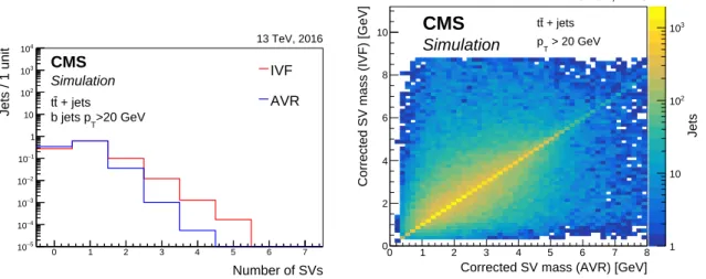
using the IVF algorithm is about 75% (12%), compared to 65% (4%) for reconstructing a sec-ondary vertex with the AVR algorithm. However, the efficiency gain is largest for c jets with an IVF secondary vertex reconstruction efficiency of about 37%, compared to 23% for the effi-ciency of the AVR algorithm. Averaged over all jet flavours, 66% of the IVF secondary vertices in jets are also found by the AVR algorithm. The other way around, 86% of the AVR secondary vertices are also found by the IVF algorithm. Figure 7 (left) compares the number of secondary vertices in b jets for the IVF and AVR algorithms. As expected, more secondary vertices are re-constructed with the IVF algorithm because of the inclusive approach of using all tracks instead

(14)

Corrected SV mass [GeV] 0 1 2 3 4 5 6 7 8 9 10 Jets / 0.2 GeV 3 − 10 2 − 10 1 − 10 1 10 b jets c jets udsg jets + jets t t > 20 GeV T p 13 TeV, 2016 CMS Simulation

SV 2D flight distance significance 0 10 20 30 40 50 60 70 80 90 100 Jets / 2 units 5 − 10 4 − 10 3 − 10 2 − 10 1 − 10 1 10 2 10 3 10 b jets c jets udsg jets + jets t t > 20 GeV T p 13 TeV, 2016 CMS Simulation

Figure 6: Distribution of the corrected secondary vertex mass (left) and of the secondary vertex 2D flight distance significance (right) for jets containing an IVF secondary vertex. The distribu-tions are shown for jets of different flavours in tt events and are normalized to unit area. The last bin includes the overflow entries.

of only those associated with the jet and passing the selection requirements. The right panel in Fig. 7 shows the correlation between the corrected mass of the secondary vertices obtained with the two approaches. From the correlation it is clear that the same secondary vertex is found in most cases. Since the efficiency of the IVF algorithm is higher, IVF secondary vertices are used to compute the secondary vertex variables for the heavy-flavour jet identification algorithms. AVR secondary vertices are only used in one of the b jet identification algorithms discussed in Section 5. Number of SVs 0 1 2 3 4 5 6 7 Jets / 1 unit 5 − 10 4 − 10 3 − 10 2 − 10 1 − 10 1 10 2 10 3 10 4 10 IVF AVR + jets t t >20 GeV T b jets p 13 TeV, 2016 CMS Simulation Jets 1 10 2 10 3 10

Corrected SV mass (AVR) [GeV]

0 1 2 3 4 5 6 7 8

Corrected SV mass (IVF) [GeV]

0 2 4 6 8 10 tt + jets > 20 GeV T p 13 TeV, 2016 CMS Simulation

Figure 7: Distribution of the number of secondary vertices in b jets for the two vertex finding algorithms described in the text (left). The distributions are normalized to unit area. Correla-tion between the corrected secondary vertex mass for the vertices obtained with the two vertex finding algorithms (right). Both panels show jets in tt events.

4.4 Soft-lepton variables

Although an electron or muon is present in only 20% (10%) of the b (c) jets, the properties of this low-energy nonisolated “soft lepton” (SL) permit the selection of a pure sample of heavy-flavour jets. Therefore, some of the heavy-heavy-flavour taggers use the properties of these soft lep-tons. Soft muons are defined as particles clustered in the jet passing the loose muon

(15)

identifica-13

tion criteria and with a pTof at least 2 GeV [10]. Electrons are associated with a jet by requiring

∆R < 0.4. Soft electrons should pass the loose electron identification criteria, have an

associ-ated track with at least three hits in the pixel layers, and be identified as not originating from a photon conversion [9].

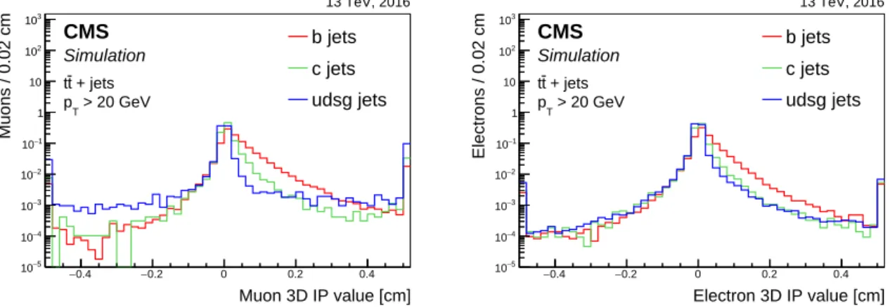
Discriminating variables using soft lepton information are typically similar to the variables based on track information alone. As an example, Fig. 8 shows the distribution of the 3D impact parameter value of soft leptons associated with jets. The 3D impact parameter value of

Muon 3D IP value [cm] 0.4 − −0.2 0 0.2 0.4 Muons / 0.02 cm 5 − 10 4 − 10 3 − 10 2 − 10 1 − 10 1 10 2 10 3 10 b jets c jets udsg jets + jets t t > 20 GeV T p 13 TeV, 2016 CMS Simulation Electron 3D IP value [cm] 0.4 − −0.2 0 0.2 0.4 Electrons / 0.02 cm 5 − 10 4 − 10 3 − 10 2 − 10 1 − 10 1 10 2 10 3 10 b jets c jets udsg jets + jets t t > 20 GeV T p 13 TeV, 2016 CMS Simulation

Figure 8: Distribution of the 3D impact parameter value for soft muons (left) and soft electrons (right) for jets of different flavours in tt events. The distributions are normalized to unit area. The first and last bins include the underflow and overflow entries, respectively.

the soft lepton discriminates between the various jet flavours. For the low-pTmuons expected

from the heavy-flavour hadron decays, it should be noted that the impact parameter resolution

is worse than at high pT [10], which is reflected in the relatively large spread of the impact

parameter values. The soft lepton variables are used in the soft lepton algorithms discussed in Section 5.1.3 and in the c tagger discussed in Section 5.2.1.

5 Heavy-flavour jet identification algorithms

5.1 The b jet identification

The jet probability (JP) and combined secondary vertex (CSV) taggers used during Run 1 [1] are also used for the Run 2 analyses. Likewise, the combined multivariate analysis (cMVA) tagger, which combines the discriminator values of various taggers, was retrained. Apart from the retraining, the CSV algorithm was also optimized and the new version is referred to as CSVv2. In addition, another version of the CSV algorithm was developed that uses deep ma-chine learning [38] (DeepCSV). These taggers are presented in more detail in the Sections 5.1.1 to 5.1.3. The new developments result in a performance that is significantly better than that of the Run 1 taggers, as discussed in Section 5.1.4.

5.1.1 Jet probability taggers

There are two jet probability taggers, the JP and JBP algorithms. The JP algorithm is described in Ref. [1] and uses the signed impact parameter significance of the tracks associated with the jet to obtain a likelihood for the jet to originate from the primary vertex. This likelihood, or jet probability, is obtained as follows. The negative impact parameter significance of tracks from light-flavour jets reflects the resolution of the measured track impact parameter values. Hence,

(16)

the distribution of the negative impact parameter significance is used as a resolution function.

The probability for a track to originate from the primary vertex, Ptr, is obtained by integrating

the resolution functionR(s)from−∞ to the negative of the absolute track impact parameter

significance,−|IP|/σ:

Ptr =

Z −|IP|/σ

−∞ R(s)ds. (1)

The resolution function depends strongly on the quality of the reconstructed track, e.g. the number of hits in the pixel and strip layers of the tracker. Moreover, the probability for a given track to originate from the primary vertex will be smaller for tracks with a large number of missing hits. Therefore, different resolution functions are defined for various track qual-ity classes. In addition, the track qualqual-ity may be different in data and simulated events. To calibrate the JP algorithm, the resolution functions are determined separately for data and sim-ulation. Using Eq. (1), tracks corresponding to particles from the decay of a displaced particle will have a low track probability, indicating that the track is not compatible with the primary

vertex. The individual track probabilities are combined to obtain a jet probability Pjas follows:

Pj =Π N−1

∑

tr=0 (−lnΠ)tr tr! , (2)

where Π is the product over the track probabilities, Ptr, and the sum runs over the selected

tracks index tr, with N the number of selected tracks associated with the jet. To avoid insta-bilities due to the multiplication of small track probainsta-bilities, the probability is set to 0.5% for track probabilities below 0.5%. Only tracks with a positive impact parameter and for which

the angular distance between the track and the jet axis satisfies∆R < 0.3 are used. A variant

of the JP algorithm also exists for which the four tracks with the highest impact parameter sig-nificance get a higher weight in the jet probability calculation. This algorithm is referred to as

jet b probability (JBP) and uses tracks with∆R < 0.4. For a light-flavour jet misidentification

probability of around 10%, the JBP algorithm has a b jet identification efficiency of 80% com-pared to 78% for the JP algorithm. The discriminators for the jet probability algorithms were

constructed to be proportional to−ln Pj. Figure 9 shows the distributions of the discriminator

values for the JP and JBP algorithms. The discontinuities in the discriminator distributions are due to the minimum track probability threshold of 0.5%.

The jet probability algorithms are interesting for two reasons. First, the fact that the calibra-tion of the resolucalibra-tion funccalibra-tion is performed independently for data and simulacalibra-tion results in a robust reference tagger. Second, these algorithms rely only on the impact parameter informa-tion of the tracks. Therefore, they are used by some methods when measuring the efficiency of other b jet identification algorithms that rely on secondary vertex or soft lepton information, as discussed in Sections 8 and 9.

5.1.2 Combined secondary vertex taggers

5.1.2.1 The CSVv2 tagger The CSVv2 algorithm is based on the CSV algorithm de-scribed in Ref. [1] and combines the information of displaced tracks with the information on secondary vertices associated with the jet using a multivariate technique. Two variants of the CSVv2 algorithm exist according to whether IVF or AVR vertices are used. As baseline, IVF vertices are used in the CSVv2 algorithm, otherwise we refer to it as CSVv2 (AVR). At least two tracks per jet are required. When calculating the values of the track variables, the tracks are

required to have an angular distance with respect to the jet axis of∆R < 0.3. Moreover, any

(17)

5.1 Theb jet identification 15 JP discriminator 0 0.5 1 1.5 2 2.5 3 Jets / 0.06 units 5 − 10 4 − 10 3 − 10 2 − 10 1 − 10 1 10 2 10 3 10 b jets c jets udsg jets + jets t t > 20 GeV T p 13 TeV, 2016 CMS Simulation JBP discriminator 0 1 2 3 4 5 6 7 8 9 Jets / 0.18 units 5 − 10 4 − 10 3 − 10 2 − 10 1 − 10 1 10 2 10 3 10 b jets c jets udsg jets + jets t t > 20 GeV T p 13 TeV, 2016 CMS Simulation

Figure 9: Distribution of the JP (left) and JBP (right) discriminator values for jets of different flavours in tt events. Jets without selected tracks are assigned a negative value. The distribu-tions are normalized to unit area. The first and last bin include the underflow and overflow entries, respectively.

is rejected. Jets that have neither a selected track nor a secondary vertex are assigned a default

output discriminator value of−1.

In a first step, the algorithm has to learn the features, e.g. input variable distributions cor-responding to the various jet flavours, and combine them into a single discriminator output value. This step is the so-called “training” of the algorithm. During this step, it is important to ensure that the algorithm does not learn any unwanted behaviour, such as b jets having a

higher jet pT, on average, compared to other jets in a sample of tt events. To avoid

discrimina-tion between jet flavours caused by different jet pT and η distributions, these distributions are

reweighted to obtain the same spectrum for all jet flavours in the training sample. The training is performed on inclusive multijet events in three independent vertex categories:

• RecoVertex: The jet contains one or more secondary vertices.

• PseudoVertex: No secondary vertex is found in the jet but a set of at least two tracks with a 2D impact parameter significance above two and a combined invariant mass

at least 50 MeV away from the K0_S mass are found. Since there is no real secondary

vertex reconstruction, no fit is performed, resulting in a reduced number of vari-ables.

• NoVertex: Containing jets not assigned to one of the previous two categories. Only the information of the selected tracks is used.

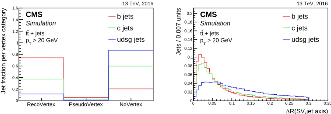
Figure 10 shows the fraction of jets of each flavour in the various vertex categories of the CSVv2

algorithm using jets in tt events with pTabove 20 GeV, where the secondary vertices in the

Re-coVertex category are obtained with the IVF algorithm. The following discriminating variables are combined in the algorithm.

• The “SV 2D flight distance significance”, defined as the 2D flight distance

signifi-cance of the secondary vertex with the smallest uncertainty on its flight distance for jets in the RecoVertex category.

• The “number of SV”, defined as the number of secondary vertices for jets in the

RecoVertex category.

• The “track ηrel”, defined as the pseudorapidity of the track relative to the jet axis for

(18)

RecoVertex PseudoVertex NoVertex

Jet fraction per vertex category

0 0.2 0.4 0.6 0.8 1 1.2 1.4 1.6 b jets c jets udsg jets + jets t t > 20 GeV T p 13 TeV, 2016 CMS Simulation R(SV,jet axis) ∆ 0 0.05 0.1 0.15 0.2 0.25 0.3 0.35 Jets / 0.007 units 0 0.02 0.04 0.06 0.08 0.1 0.12 0.14 0.16 0.18 0.2 b jets c jets udsg jets + jets t t > 20 GeV T p 13 TeV, 2016 CMS Simulation

Figure 10: Vertex category for secondary vertices reconstructed with the IVF algorithm (left), and the distribution of the angular distance between the IVF secondary vertex flight direction and the jet axis (right) for jets of different flavours in tt events. The distributions are normalized to unit area.

and PseudoVertex categories.

• The “corrected SV mass”, defined as the corrected mass of the secondary vertex with

the smallest uncertainty on its flight distance for jets in the RecoVertex category or the invariant mass obtained from the total summed four-momentum vector of the selected tracks for jets in the PseudoVertex category.

• The “number of tracks from SV”, defined as the number of tracks associated with

the secondary vertex for jets in the RecoVertex category or the number of selected tracks for jets in the PseudoVertex category.

• The “SV energy ratio”, defined as the energy of the secondary vertex with the

small-est uncertainty on its flight distance divided by the energy of the total summed four-momentum vector of the selected tracks.

• The “∆R(SV, jet)”, defined as the∆R between the flight direction of the secondary

vertex with the smallest uncertainty on its flight distance and the jet axis for jets

in the RecoVertex category, or the ∆R between the total summed four-momentum

vector of the selected tracks for jets in the PseudoVertex category.

• The “3D IP significance of the first four tracks”, defined as the signed 3D impact

parameter significances of the four tracks with the highest 2D impact parameter significance.

• The “track pT,rel”, defined as the track pTrelative to the jet axis, i.e. the track

momen-tum perpendicular to the jet axis, for the track with the highest 2D impact parameter significance.

• The “∆R(track, jet)”, defined as the ∆R between the track and the jet axis for the

track with the highest 2D impact parameter significance.

• The “track pT,relratio”, defined as the track pT relative to the jet axis divided by the

magnitude of the track momentum vector for the track with the highest 2D impact parameter significance.

• The “track distance”, defined as the distance between the track and the jet axis at

their point of closest approach for the track with the highest 2D impact parameter significance.

(19)

5.1 Theb jet identification 17

the track at the point of closest approach between the track and the jet axis for the track with the highest 2D impact parameter significance.

• The “summed tracks ETratio”, defined as the transverse energy of the total summed

four-momentum vector of the selected tracks divided by the transverse energy of the jet.

• The “∆R(summed tracks, jet)”, defined as the∆R between the total summed

four-momentum vector of the tracks and the jet axis.

• The “first track 2D IP significance above c threshold”, defined as the 2D impact

pa-rameter significance of the first track that raises the combined invariant mass of the tracks above 1.5 GeV. This track is obtained by summing the four-momenta of the tracks adding one track at the time. Every time a track is added, the total four-momentum vector is computed. The 2D impact parameter significance of the first track that is added resulting in a mass of the total four-momentum vector above the aforemention threshold is used as a variable. The threshold of 1.5 GeV is related to the c quark mass.

• The number of selected tracks.

• The jet pT and η.

The discriminating variables in each vertex category are combined into a neural network, specifically a feed-forward multilayer perceptron with one hidden layer [39]. The number of nodes in the hidden layer is different for the three different vertex categories and is set to twice the number of input variables. The discriminator values of the three vertex categories are com-bined with a likelihood ratio taking into account the fraction of jets of each flavour expected in

tt events. The fraction of jets of each flavour is obtained as a function of the jet pTand|η|, using

19 exclusive bins in total. Two dedicated trainings are performed, one with c jets, and one with light-flavour jets as background. The final discriminator value is a linear combination of the output of these two trainings with relative weights of 1 : 3 for the output of the network trained against c and light-flavour jets, respectively. The value of these relative weights is inspired by tt events where one of the two W bosons decays into quarks and the other into leptons, and provides the best performance for a wide variety of physics topologies compared to alternative relative weights.

The main differences from the Run 1 version of the CSV algorithm are the following:

• The secondary vertex reconstruction algorithm: The secondary vertices are recon-structed with the IVF algorithm.

• Input variables: Table 1 lists the variables used for the Run 1 version of the CSV algorithm and for the CSVv2 algorithm. Figure 11 shows two of the variables used for the CSVv2 algorithm and not for the CSV algorithm.

• Multilayer perceptron: In the previous version of the algorithm the input variables in a certain vertex category were combined with a likelihood ratio. Depending on the type of correlations present between the input variables, the likelihood ratio per-forms at a comparable level to the other multivariate methods. The likelihood ratio is particularly useful because of its simplicity and when a small number of variables are used. However, to increase the performance of the algorithm, more input vari-ables were added and combined into an artificial neural network.

• Jet pT and η dependence: The correlation of some of the input variables with the

jet pT and η is taken into account by including the jet kinematics as input variables,

(20)

the training was performed in bins of the jet kinematics. In the current procedure, the bins of jet kinematics are only used to combine the vertex categories after the training.

Table 1: Input variables used for the Run 1 version of the CSV algorithm and for the CSVv2 algorithm. The symbol “x” (“—”) means that the variable is (not) used in the algorithm

Input variable Run 1 CSV CSVv2

SV 2D flight distance significance x x

Number of SV — x

Track ηrel x x

Corrected SV mass x x

Number of tracks from SV x x

SV energy ratio x x

∆R(SV, jet) — x

3D IP significance of the first four tracks x x

Track p_T,rel — x

∆R(track, jet) — x

Track pT,relratio — x

Track distance — x

Track decay length — x

Summed tracks ETratio — x

∆R(summed tracks, jet) — x

First track 2D IP significance above c threshold — x

Number of selected tracks — x

Jet pT — x

Jet η — x

Figure 12 shows the distribution of the discriminator values for the various jet flavours for both versions of the CSVv2 algorithm.

5.1.2.2 The DeepCSV tagger The identification of jets from heavy-flavour hadrons can be improved by using the advances in the field of deep machine learning [38]. A new version of the CSVv2 tagger, “DeepCSV”, was developed using a deep neural network with more hidden layers, more nodes per layer, and a simultaneous training in all vertex categories and for all jet flavours.

The same tracks and IVF secondary vertices are used in this approach as for the CSVv2 tagger. The same input variables are also used, with only one difference, namely that for the track-based variables up to six tracks are used in the training of the DeepCSV. Jets are randomly

selected in such a way that similar jet pT and η distributions are obtained for all jet flavours.

These jet pT and η distributions are also used as input variables in the training to take into

account the correlation between the jet kinematics and the other variables. The distribution of all input variables is preprocessed to centre the mean of each distribution around zero and to obtain a root-mean-square value of unity. All of the variables are presented to the multivariate analysis (MVA) in the same way because of the preprocessing. This speeds up the training. In case a variable cannot be reconstructed, e.g. because there are less than six selected tracks (or no secondary vertex), the variable values associated with the missing track or vertex are set to zero after the preprocessing.

The training is performed using jets with pTbetween 20 GeV and 1 TeV, and within the tracker

(21)

5.1 Theb jet identification 19 (jet) T )) / E p (E, trk Σ ( T E 0 0.1 0.2 0.3 0.4 0.5 0.6 0.7 0.8 0.9 1 Jets / 0.02 units 0 0.01 0.02 0.03 0.04 0.05 0.06 0.07 b jets c jets udsg jets + jets t t > 20 GeV T p 13 TeV, 2016 CMS Simulation R(track,jet axis) ∆ 0 0.05 0.1 0.15 0.2 0.25 0.3 0.35 Tracks / 0.007 units 0 0.01 0.02 0.03 0.04 0.05 0.06 0.07 0.08 0.09 0.1 b jets c jets udsg jets + jets t t > 20 GeV T p 13 TeV, 2016 CMS Simulation

Figure 11: Distribution of the transverse energy of the total summed four-momentum vector of the selected tracks divided by the jet transverse energy (left), and angular distance between the track and the jet axis (right) for jets of different flavours in tt events. The distributions are normalized to unit area. The last bin in the left panel includes the overflow entries.

CSVv2 discriminator 0 0.1 0.2 0.3 0.4 0.5 0.6 0.7 0.8 0.9 1 Jets / 0.02 units 5 − 10 4 − 10 3 − 10 2 − 10 1 − 10 1 10 2 10 3 10 b jets c jets udsg jets + jets t t > 20 GeV T p 13 TeV, 2016 CMS Simulation CSVv2 (AVR) discriminator 0 0.1 0.2 0.3 0.4 0.5 0.6 0.7 0.8 0.9 1 Jets / 0.02 units 5 − 10 4 − 10 3 − 10 2 − 10 1 − 10 1 10 2 10 3 10 b jets c jets udsg jets + jets t t > 20 GeV T p 13 TeV, 2016 CMS Simulation

Figure 12: Distribution of the CSVv2 (left) and CSVv2(AVR) (right) discriminator values for jets of different flavours in tt events. The distributions are normalized to unit area. Jets without a selected track and secondary vertex are assigned a negative discriminator value. The first bin includes the underflow entries.

(22)

udsg jets. A mixture of tt and multijet events is used to reduce the possible dependency of the training on the heavy-flavour quark production process.

The training of the deep neural network is performed using the KERAS [40] deep learning

library, interfaced with the TENSORFLOW[41] library that is used for low-level operations such

as convolutions. The neural network uses four hidden layers that are fully connected, each with 100 nodes. Increasing the number of hidden layers and the number of nodes per layer had negligible effects on the performance. Each node in one of the hidden layers uses a rectified linear unit as its activation function to define the output of the node given the input values. For the nodes in the last layer, a normalized exponential function is used for the activation to be able

to interpret the output value as a probability for a certain jet flavour category, P(f). The output

layer contains five nodes corresponding to five jet flavour categories used in the training. These categories are defined according to whether the jet contains exactly one b hadron, at least two b hadrons, exactly one c hadron and no b hadrons, at least two c hadrons and no b hadrons, or none of the aforementioned categories. Each of these categories is completely independent of the others. The reason for defining five flavour categories in the training is to provide analyses with the possibility to identify jets containing two b or c hadrons.

Figure 13 shows the discriminator distribution for each of the DeepCSV probabilities P(f).

The lower right panel in Fig. 13 also shows the P(b) +P(bb)discriminator used to tag b jets in

physics analyses. It has been checked that summing the probabilities for these two categories is equivalent to using a combined training for these categories.

5.1.3 Soft-lepton and combined taggers

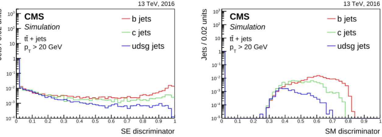
Soft leptons, i.e. electrons or muons reconstructed as described in Section 4.4 are sometimes present in a jet. When they are, the information related to the charged lepton is used to con-struct a soft-electron (SE) and soft-muon (SM) tagger. The discriminating variables that are used as input for the boosted decision tree (BDT) are the 2D and 3D impact parameter

signifi-cance of the lepton, the angular distance between the jet axis and the lepton,∆R, the ratio of the

pTof the lepton to that of the jet, and the pTof the lepton relative to the jet axis, prelT . In the case

of the SE algorithm an MVA-based electron identification variable is also used as input. The distributions of the SE and SM discriminator values are shown in Fig. 14. The different range for the algorithm output values is related to different settings in the training when combining the input variables with a BDT.

As a soft lepton is only present in a relatively small fraction of heavy-flavour jets, the soft lepton taggers are not always able to discriminate heavy-flavour jets from other jets. Therefore they are not used standalone, but rather as input for a combined tagger. The combined tagger, cMVAv2, uses six b jet identification discriminators as input variables, namely the two variants of the JP algorithm, the SE and SM algorithms, and the two variants of the CSVv2 algorithm. The

training is performed using the open sourceSCIKIT-LEARNpackage [42] and the variables are

combined using a gradient boosting classifier (GBC) as BDT. Prior to the training, the jet pTand

ηdistributions are reweighted to obtain a similar distribution for all jet flavours. Although the

correlation between the two CSVv2 discriminator values is close to 100%, a small improvement is seen in the case where the vertex finding algorithms reconstruct different secondary vertices. Figure 15 shows the correlation between the input variables of the cMVAv2 algorithm for b jets as well as the distribution of the cMVAv2 discriminator values for various jet flavours obtained in a tt sample. The correlation between the input variables is similar for other jet flavours. Adding the SL taggers or one of the JP taggers as input variables for the cMVAv2 algorithm results in a similar large performance gain with respect to the CSVv2 algorithm.

(23)

5.1 Theb jet identification 21 DeepCSV P(b) discriminator 0 0.1 0.2 0.3 0.4 0.5 0.6 0.7 0.8 0.9 1 Jets / 0.02 units 5 − 10 4 − 10 3 − 10 2 − 10 1 − 10 1 10 2 10 3 10 b jets c jets udsg jets + jets t t > 20 GeV T p 13 TeV, 2016 CMS Simulation DeepCSV P(bb) discriminator 0 0.1 0.2 0.3 0.4 0.5 0.6 0.7 0.8 0.9 1 Jets / 0.02 units 5 − 10 4 − 10 3 − 10 2 − 10 1 − 10 1 10 2 10 3 10 b jets c jets udsg jets + jets t t > 20 GeV T p 13 TeV, 2016 CMS Simulation DeepCSV P(c) discriminator 0 0.1 0.2 0.3 0.4 0.5 0.6 0.7 0.8 0.9 1 Jets / 0.02 units 5 − 10 4 − 10 3 − 10 2 − 10 1 − 10 1 10 2 10 3 10 b jets c jets udsg jets + jets t t > 20 GeV T p 13 TeV, 2016 CMS Simulation DeepCSV P(cc) discriminator 0 0.1 0.2 0.3 0.4 0.5 0.6 0.7 0.8 0.9 1 Jets / 0.02 units 5 − 10 4 − 10 3 − 10 2 − 10 1 − 10 1 10 2 10 3 10 b jets c jets udsg jets + jets t t > 20 GeV T p 13 TeV, 2016 CMS Simulation

DeepCSV P(udsg) discriminator 0 0.1 0.2 0.3 0.4 0.5 0.6 0.7 0.8 0.9 1 Jets / 0.02 units 5 − 10 4 − 10 3 − 10 2 − 10 1 − 10 1 10 2 10 3 10 b jets c jets udsg jets + jets t t > 20 GeV T p 13 TeV, 2016 CMS Simulation DeepCSV P(b)+P(bb) discriminator 0 0.1 0.2 0.3 0.4 0.5 0.6 0.7 0.8 0.9 1 Jets / 0.02 units 5 − 10 4 − 10 3 − 10 2 − 10 1 − 10 1 10 2 10 3 10 b jets c jets udsg jets + jets t t > 20 GeV T p 13 TeV, 2016 CMS Simulation

Figure 13: Distribution of the DeepCSV P(b)(upper left), P(bb)(upper right), P(c)(middle

left), P(cc)(middle right), P(udsg)(lower left), and P(b) +P(bb)(lower right) discriminator

values for jets of different flavours in tt events. Jets without a selected track and without a secondary vertex are assigned a discriminator value of 0. The distributions are normalized to unit area.

(24)

SE discriminator 0 0.1 0.2 0.3 0.4 0.5 0.6 0.7 0.8 0.9 1 Jets / 0.02 units 4 − 10 3 − 10 2 − 10 1 − 10 1 10 2 10 3 10 b jets c jets udsg jets + jets t t > 20 GeV T p 13 TeV, 2016 CMS Simulation SM discriminator 0 0.1 0.2 0.3 0.4 0.5 0.6 0.7 0.8 0.9 1 Jets / 0.02 units 5 − 10 4 − 10 3 − 10 2 − 10 1 − 10 1 10 2 10 3 10 b jets c jets udsg jets + jets t t > 20 GeV T p 13 TeV, 2016 CMS Simulation

Figure 14: Distribution of the soft-electron (left) and soft-muon (right) discriminator values for jets of different flavours in tt events. Jets without a soft lepton are assigned a discriminator value of 0. The distributions are normalized to unit area.

Adding the other JP tagger and CSVv2 (AVR) algorithm results only in a modest performance gain. The performance of the cMVAv2 tagger for discriminating b jets against other jet flavours is discussed more extensively in Section 5.1.4.

1.00 0.03 0.07 0.08 0.04 0.03 0.03 1.00 0.35 0.37 0.29 0.27 0.07 0.35 1.00 0.90 0.66 0.70 0.08 0.37 0.90 1.00 0.70 0.72 0.04 0.29 0.66 0.70 1.00 0.96 0.03 0.27 0.70 0.72 0.96 1.00 SE SM CSVv2 (IVF)CSVv2 (AVR)JP JBP SE SM CSVv2 (IVF) CSVv2 (AVR) JP JBP

Linear correlation coefficient

0 0.1 0.2 0.3 0.4 0.5 0.6 0.7 0.8 0.9 1 + jets t t > 20 GeV T b jets p 13 TeV, 2016 CMS Simulation cMVAv2 discriminator 1 − −0.8 −0.6 −0.4 −0.2 0 0.2 0.4 0.6 0.8 1 Jets / 0.04 units 4 − 10 3 − 10 2 − 10 1 − 10 1 10 2 10 3 10 b jets c jets udsg jets + jets t t > 20 GeV T p 13 TeV, 2016 CMS Simulation

Figure 15: Correlation between the different input variables for the cMVAv2 tagger for b jets in tt events (left), and distribution of the cMVAv2 discriminator values (right), normalized to unit area, for jets of different flavours in tt events.

It is relevant to note that the DeepCSV discriminator output was not included as an input variable, as this algorithm was developed after the cMVAv2 tagger. Further optimizations are ongoing, in particular in the context of the new pixel tracker installed in 2017 [43].

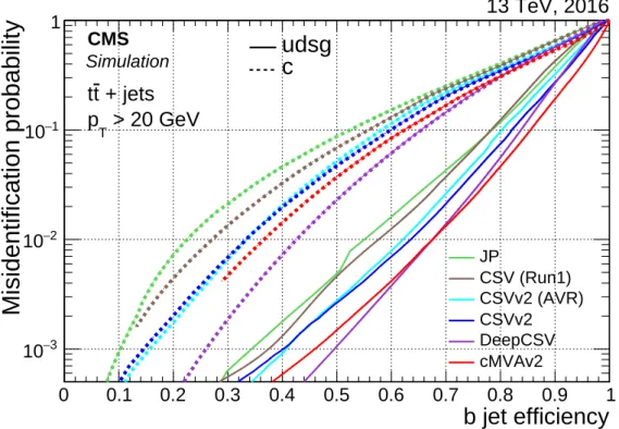
5.1.4 Performance in simulation

The tagging efficiency of the JP, CSVv2, cMVAv2, and DeepCSV taggers is determined us-ing simulated pp collision events. The efficiency (misidentification probability) to correctly (wrongly) tag a jet with flavour f is defined as the number of jets of flavour f passing the tagging requirement divided by the total number of jets of flavour f . Figure 16 shows the b jet identification efficiency versus the misidentification probability for either c or light-flavour