1
Equity Valuation of Under Armour
Rafael Diogo
Dissertation written under the supervision of José Carlos Tudela
Martins
Dissertation submitted in partial fulfilment of requirements for the
International MSc in Management – Major in Corporate Finance, at
2 Table of Contents
Abstract ... 4
Abstract (versão portuguesa) ... 5
Under Armour – Investment note ... 6
1. Introduction ... 7
2. Literature Review ... 8
2.1. Valuation Purpose and Tools ... 8
2.2. Enterprise Value Methods ... 8
2.2.1. Cash Flow Approach - Discounted Cash Flow (DCF) ... 8
2.2.1.1. Terminal Value and stable state ... 9
2.2.1.2. Terminal Value Growth Rate ... 10
2.2.1.3. Required Return to Equity – 𝒌𝒆 ... 10
2.2.1.4. Risk-Free Rate ... 11
2.2.1.5. Market Risk Premium, Small Minus Big and High Minus Lows ... 12
2.2.1.6. DCF – Weighted Average Cost of Capital (WACC) ... 13
2.2.1.7. DCF – Adjusted Present Value (APV) ... 14
2.2.1.8. Present Value of Tax Shields ... 15
2.2.1.9. Expected Costs of Financial Distress ... 16
2.2.2. Returns Based Approach – Economic Value Added (EVA) ... 17
2.3. Equity Methods ... 18
2.3.1. Cash Flow Approach – Dividend Discount Model (DDM) ... 18
2.4. Multiples/Relative Approaches ... 20 2.5. Conclusion ... 21 3. Company Overview ... 23 4. Industry Overview ... 24 4.1. Macro Analysis ... 24 4.2. Micro Analysis ... 26
5. Valuation Inputs– APV ... 29
5.1. Revenue estimation... 29
5.2. Cost of Goods Sold / Gross Margin ... 30
5.3. Selling, General and Administrative Expense ... 31
5.4. Debt Outstanding and Interest Expense ... 33
5.5. Other expense ... 33
5.6. Effective tax-rate ... 34
3
5.8. Capitalizing R&D ... 34
5.9. Capitalizing Operating Leases ... 35
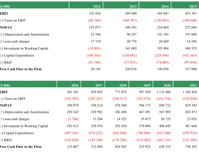
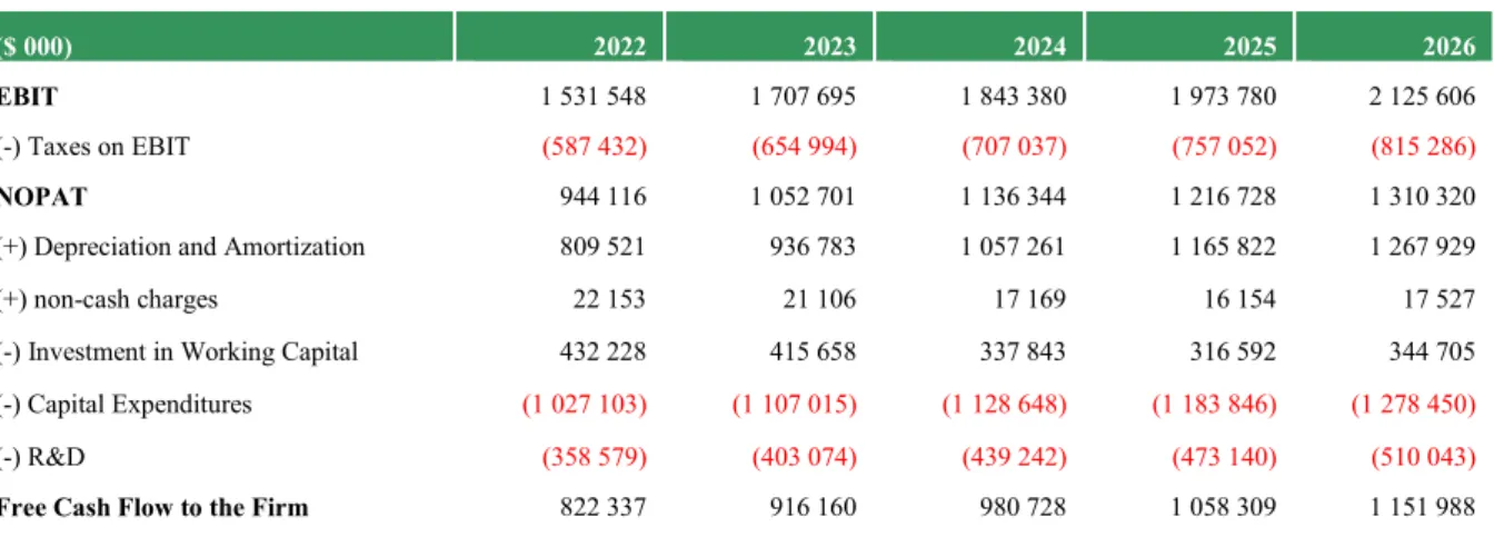
5.10. Free Cash Flows to the firm ... 35
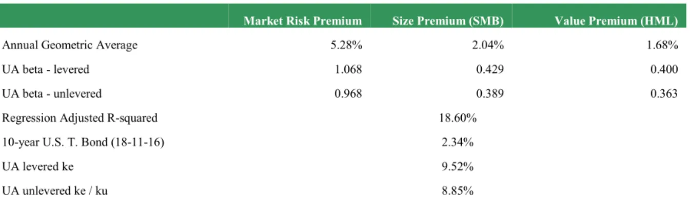
5.11. Required Return to Equity ... 36
5.12. Long-term growth rate ... 37
6.Valuation Exercise – APV ... 37
6.1. Base-Case ... 37
6.2. PV of Tax-Shields ... 38
6.3. Costs of Financial Distress ... 38
6.4. From Enterprise Value to Share Value ... 38
7. Valuation Exercise – DDM ... 40
8. Valuation Exercise – Relative Valuation ... 41
9. Comparison with The Buckingham Research Group Valuation Model ... 43
10. Conclusion ... 44
11. Appendix Section ... 45
12. List of Figures, Graphs and Tables ... 74
4 Abstract
The present dissertation is intended to present a valuation for Under Armour – a sportswear company that has experienced incredible growth in the recent past.
Under Armour represents a story of entrepreneurship, focus and greatness, personalized by the founder and current CEO. Kevin Plank created the company in 1996, when he was only 23 years old, in the form of a t-shirt prototype. Since then, the company has experienced an IPO in 2005 and revealed consistent and extreme revenue growth and has been able to expand its operations worldwide.
Three different valuation models were applied, with the objective to find a range of values in which UA stock’s intrinsic value currently falls. The present valuation is also compared with an external one made by an equity research firm – The Buckingham Research Group. This comparison should contribute in giving the reader extra perspective regarding the valuation’s methodology and output.
After both processes, an investment note was issued, with a Buy recommendation and a target price of $37 per share for the Class A common stock.
5 Abstract (versão portuguesa)
A dissertação aqui apresentada tem como objetivo apresentar uma avaliação para a Under Armour, - empresa que desenvolve a sua atividade na indústria do equipamento desportivo. A Under Armour representa um exemplo de empreendedorismo, determinação e excelência, personalizada pelo seu fundador e atual diretor executivo. Kevin Plank criou a empresa em 1996, com apenas 23 anos, através do desenvolvimento de um protótipo de uma t-shirt desportiva. Entretanto, a empresa já experienciou uma OPA em 2005 e tem revelado um crescimento exponencial e consistente em termos de receitas, tendo conseguido expandir as suas operações a um nível global.
Três modelos diferentes de avaliação foram usados nesta dissertação, com o objetivo de encontrar um intervalo de valores, no qual o valor intrínseco das ações da Under Armour se encontrarão. A avaliação realizada foi ainda comparada com uma outra avaliação externa, desenvolvida por uma empresa especializada na área da avaliação financeira – The Buckingham Research Group. Pretendeu-se, assim, possibilitar uma perspetiva mais alargada ao leitor, quer quanto aos métodos usados na avaliação, quer quanto aos seus resultados.
Concluídos todos estes procedimentos, de acordo com a metodologia explanada, foi feita uma nota de investimento, com a recomendação de Buy e um preço-alvo de $37 para as ações “Class A” da Under Armour.
6 Under Armour – Investment note
Market Overreaction; High-growth to be maintained;
Recommendation: BUY; Target Price: UAA: $37; UA.C: $32
After years of overperformance, Under Armour’s shares plummeted by 15% after the market opening. The reason for the fall was the company’s announcement that the consistent high growth of over 20%, lasting for 26 quarters prior to that date, would finally slow down.
At the time, such developments were unexpected and several analysts placed the company’s target price in the $40 to $50 range. The market reacted instantly, both to the revenue growth deceleration announcement, as to the margin operating margin tightening that was felt in the current year.
Nevertheless, the present valuation shows that even with the high competition felt in the market, causing the gross and operating margins to stay at lower levels than in the recent past, UA’s financials value the company at 26% above market valuation, under the APV and Relative Valuations. A low-twenty’s revenue growth, as announced by UA, together with the maintenance of the current levels of capital expenditures, R&D and marketing costs (which may be interpreted as conservative) still return higher valuations than the market does.
The present analysis holds a BUY recommendation, maintaining confidence that the market overreacted to the company announcements, and that within 6-12 months it will revalue the company at higher levels than the current $29.42.
Recommendation:
BUY
UAA – Class A common stock Target Price:
$37.04-$37.07
Stock Price as of 28-12-2016: $29.42
UA.C – Class C common stock Target Valuation Range: $31.76-$31.78
Stock Price as of 28-12-2016: $25.41
Valuation Outputs - UAA
APV $37.07 EV/EBITDA $37.04 DDM $27.67 Upside/Downside Potential: APV – 26.00% EV/EBITDA – 25.90% DDM – (5.93%)
The Buckingham Research Group: Date: 20-06-2016
Recommendation: BUY Target Price: $48
Key Management:
Kevin Plank Lawrence Molloy
7 1. Introduction
The aim of this master thesis is to reach a valuation for the equity of Under Armour Inc, and one that is as close as possible to its intrinsic value.
As a definition, “a stock’s intrinsic value is the present value of its expected future dividends (or cash flows) to common shareholders” (Lee, Myers, & Swaminathan, 1999). The determination of such cash flows is far from being an exact task. Either when performing the valuation or when appreciating a valuation made by someone else, one should bear in mind that “Valuation is neither the science…nor the objective search for true value that idealists would like it to become” (Damodaran, Investment Valuation, 2002).
The following valuation is, naturally, based on quantitative models and figures, but also subject to my own interpretations of all available information regarding Under Armour Inc, the industry in which it is included and the group of wider economic facts that have or will have influence over the firm’s operations and, consequently, their value.
In case there are expectations about reading this valuation and arriving at a specific value that should be taken as the stock’s correct price, readers should leave them behind. Instead, the values arrived at should be viewed more as a range within which the stock price should lay. To have a better perspective of the validity of this valuation, one other analysis made by active professionals in equity research is taken as a comparison. Differences, both in values as in methods of valuation, among the two different studies, will be scrutinized and explained in this report as well. The comparative analysis chosen was made by The Buckingham Research Group Incorporated, a financial service firm, specialized in “value-add” equity research and based in New York.
In terms of structure, the first sub-topic will be dedicated to a review of the existing literature regarding equity valuation. The literature taken into consideration for this effect is a state of the art set of articles and books, present in top academic journals or top firms in the activity of equity valuation. The second section will be focused on Under Armour Inc’s company and industry overview. The third segment will contain the presentation of the valuation per se, arising from the different methods chosen. The final part of the repost will be devoted to the comparison between the valuation referred and the one from The Buckingham Research Group Incorporated, and to an explanation of the differences and similarities among both.
8 2. Literature Review
2.1. Valuation Purpose and Tools
An equity valuation process may have three different applications. The first one is Portfolio Management. Within Portfolio Management, the philosophies behind each investment and the types of investment made vary quite a lot.
The second possible application happens in the case of a Merger or Acquisition. In such circumstances, “The bidding firm or individual has to decide on a fair value for the target firm before making a bid, and the target firm has to determine a reasonable value for itself before deciding to accept or reject the offer” (Damodaran, Investment Valuation, 2002).
The third application of a valuation analysis is linked with Corporate Finance. “If the objective in corporate finance is the maximization of firm value, the relationship among financial decisions, corporate strategy and firm value has to be delineated.” (Damodaran, Investment Valuation, 2002).
In terms of methods, each valuation approach enters one of two categories: Equity Value Methods and Enterprise Value Methods. “Equity valuation approaches estimate the value of a firm to equity holders, whereas Enterprise value approaches assess the whole enterprise, the equity and the debt.” (Young, Sullivan, Nokhasteh, & Holt, 1999).
One other variance among methods is “whether the approach is based on cash flows, returns or multiples.” (Young, Sullivan, Nokhasteh, & Holt, 1999). While the first type uses the present value of future cash flows to value the object, the second one focuses on the spread between the returns on capital and its cost. The last type, multiples-based, is also often called Relative Valuation. In this method, “the value of an asset is derived from the pricing of ‘comparable’ assets, standardized using a common variable such as earning, cash flows, book-value or revenues." (Damodaran, Investment Valuation, 2002).
2.2. Enterprise Value Methods
2.2.1. Cash Flow Approach - Discounted Cash Flow (DCF)
The Discounted Cash Flow method considers the object of valuation to be “a series of risky cash flows stretching into the future.” (Luehrman, What's it Worth? A General Manager's Guide to Valuation, 1997).
9
In a DCF analysis, the cash flows take the shape of Free Cash Flows to the Firm (FCFF), defined as “the hypothetical equity cash flow when the company has no debt.” (Fernández, 2010). The formula that shall be used to calculate them is:
𝐹𝐶𝐹𝐹 = 𝐸𝐵𝐼𝑇 (1 − 𝑇) + 𝐷𝑒𝑝𝑟𝑒𝑐𝑖𝑎𝑡𝑖𝑜𝑛 − ∆𝑁𝑒𝑡 𝑊𝑜𝑟𝑘𝑖𝑛𝑔 𝐶𝑎𝑝𝑖𝑡𝑎𝑙 − 𝐶𝐴𝑃𝐸𝑋 , Where T equals the company’s tax rate. In the case of Multinational companies, such as the one in which this valuation focuses, the correct tax rate to be applied to future income may be the effective tax rate, if it has been consistent in the years prior to the valuation. The justification is that this effective tax rate may be the result of the company being taxed differently in the countries it operates, for different incomes.
The DCF formula with the Free Cash Flows will then stand as:
𝑃𝑟𝑒𝑠𝑒𝑛𝑡 𝑉𝑎𝑙𝑢𝑒 = ∑𝐸𝑥𝑝𝑒𝑐𝑡𝑒𝑑 (𝐹𝑟𝑒𝑒 𝐶𝑎𝑠ℎ 𝐹𝑙𝑜𝑤 𝑡𝑜 𝐹𝑖𝑟𝑚)𝜏 (1 + 𝑘)𝜏
𝑛
𝑡=0
2.2.1.1. Terminal Value and stable state
In the DCF method, one important rationale is that, at a given point in time, the firm enters a stable state. The analyst is supposed to estimate the FCFs until that time horizon. This period is often called the “forecast period” and it “should be as long as one can expect abnormal profitability or growth to be maintained” (Schill, 2013). The forecast period is finite also for a practicality reason: “…business will continue after the horizon, but it’s not practical to forecast free cash flow year by year to infinity.” (Brealey, Myers, & Allen, 2014).
After some time, growth is expected to converge from abnormal to stable, since “Positive abnormal profitability attracts expansion and entry into the industry sufficient to put pressure in expected returns until they drop to meet the cost of capital” (Schill, 2013). This next state may be designated as “stable state” - a period in which the company is expected to remain qualitatively similar year after year.
The formula shown above for the Discounted Cash Flow, after including the concept of terminal value, transforms into the following:
𝑃𝑟𝑒𝑠𝑒𝑛𝑡 𝑉𝑎𝑙𝑢𝑒 = ∑𝐸𝑥𝑝𝑒𝑐𝑡𝑒𝑑 (𝐹𝑟𝑒𝑒 𝐶𝑎𝑠ℎ 𝐹𝑙𝑜𝑤 𝑡𝑜 𝐹𝑖𝑟𝑚)𝜏 (1 + 𝑘)𝜏 𝜏=𝑛 𝜏=0 + 𝑇𝑒𝑟𝑚𝑖𝑛𝑎𝑙 𝑉𝑎𝑙𝑢𝑒𝑛 (1 + 𝑘)𝑛 Although there are several approaches to compute terminal value, in this valuation the one applied will be the Stable Growth Model approach, represented by the formula:
10
𝑇𝑒𝑟𝑚𝑖𝑛𝑎𝑙 𝑉𝑎𝑙𝑢𝑒𝑡 =
𝐹𝑟𝑒𝑒 𝐶𝑎𝑠ℎ 𝐹𝑙𝑜𝑤 𝑡𝑜 𝐹𝑖𝑟𝑚𝑡+1
𝑘 − 𝑔 ,
Where 𝑔 will be the Terminal Value Growth Rate.
2.2.1.2. Terminal Value Growth Rate
One fact that contributes to the importance of this measurement is the proportion of terminal value to the total value reached in a valuation using the DCF method, since “findings are that the terminal value is on average 94% of the total value if we make three annual forecasts, 90% of the total if we assume five annual forecasts and 79% of the total if we assume ten annual forecasts.” (Young, Sullivan, Nokhasteh, & Holt, 1999).
The definition of the long-term growth rate depends enormously on one factor - the growth rate of the economy into which it is comprised “since no firm can grow forever at a rate higher than the growth rate of the economy in which it operates, the constant growth rate cannot be greater than the overall growth rate of the economy.” (Damodaran, Investment Valuation, 2002). Schill (2013), also argues that if this did not happen, business operations would end up exceeding the size of the world economy at some point in the future. This upper bound should be either the global economic growth – if the company has no limitations to operate worldwide, or the national economic growth – if the company is expected to work only at a national level.
2.2.1.3. Required Return to Equity – 𝒌𝒆
The required return to equity is a term that designates the corresponding return that the market attributes, or the shareholders expect, to a certain level of risk.
The first major contribution into trying to reach the correct way to calculate 𝑘𝑒 came in the shape of the Capital Asset Pricing Model (CAPM), which Sharpe (1964) presented. The model stated that the market presented investors two pricing factors: “the price of time, or the pure interest rate … and the price of risk, the additional expected return per unit of risk borne” (Sharpe, 1964). This second type of risk, however, had a specific condition – “only systematic risks, i.e. risks to which many securities are exposed, can fetch a non-zero price” (Bodnar, Dumas, & Marston, 2003). The CAPM model states that the only risk which is not diversifiable and, thus, the only one which is rewarded to investors by the market for taking it, is the world stock market price risk - the “risk of covariation of the stock with the broader equity market” (Bodnar, Dumas, & Marston, 2003).
11
Following former academics [ (Banz, 1981), (Basu, 1983), (Rosenberg, Reid, & Lanstein, 1985), (Lakonishok, Shleifer, & Vishny, 1994)], Fama and French (1996) proposed a multifactor model that tried to explain observations of pricing by the market in a better way. This model, besides exposure to the world equity market risk, also incorporates two other factors, “the difference between the return on a portfolio of small stocks and the return on a portfolio of large stocks (SMB, small minus big); and the difference between the return on a portfolio of high-book-to-market stocks and the return on a portfolio of low-book-to-market-stocks (HML, high minus low)” (Fama & French, 1996). The model was basically built in the assumption that stock returns contained both a systematic and a specific factor. The 3-factor model stands as follows:
𝐸(𝑅𝑖) = 𝑟𝑓 + 𝛽𝑖 ∗ [𝐸(𝑅𝑚) − 𝑟𝑓] + 𝑆𝑖 ∗ 𝐸(𝑆𝑀𝐵) + 𝐻𝑖 ∗ 𝐸(𝐻𝑀𝐿)
Since this model “captures much of the variation in the cross-section of average stock returns, and it absorbs most of the anomalies that have plagued the CAPM” (Fama & French, 1996), it seems to be a better model than the classical CAPM. One evidence of the model’s quality is the finding that regressions using it tend to have a higher average R-squared measurement, which transmits the percentage of variations in the dependent variable that are explained by the variations in the independent variables.
For this reason, this valuation will use the Fama-French 3 Factor model to reach the required return to equity of the company. One last important detail is that the concept of Full Segmentation from Bodnar, Dumas and Marston (2003) will be assumed to be true in the estimation of the required return to equity shareholders of Under Armour Inc, so the factors used will be taken from the company’s domestic financial market.
2.2.1.4. Risk-Free Rate
The risk-free rate plays an important part in valuation, particularly in calculating the required return to equity holders.
Damodaran states two conditions for an investment to be risk-free: the absence of default risk and the absence of reinvestment risk. The first condition rules out any corporate securities, leaving only government securities. The second condition is linked to the timing of the investment. The utopian way to use the risk-free rate would be using year-specific risk-free rates. However, “the present value effect of using year-specific risk-free rates tends to be small”
12
(Damodaran, Investment Valuation, 2002) comparing to using a risk-free proxy with the duration of the where the duration of the cash flows in the analysed.
One other important factor referred by the author is the currency in which the risk-free proxy is emitted as “the risk-free rate used to come up with expected returns should be measured consistently with how the cash flows are measured” (Damodaran, Investment Valuation, 2002). Concluding, Damodaran (Investment Valuation, 2002) advises the use of the government bond with the lowest default risk possible (ideally zero), which has same currency as the measured cash flows, as a proxy for the risk-free rate.
2.2.1.5. Market Risk Premium, Small Minus Big and High Minus Lows
The main methods for estimating the Market Risk Premium are well summarized in Zenner, Hill, Clark and Mago (2008). Two methods try to connect dividends with the MRP. As already referred, paying dividends is currently a very politicized decision so the dividend discount and dividend yield methods will not be used in this valuation.
Another method tries to measure a portfolio’s excess return per unit of risk – the constant Sharpe Ratio method. Since it assumes that this ratio remains constant but there is “some evidence that the Sharpe ratio will change over time” (Zenner, Hill, Clark, & Mago, 2008) this approach is also abandoned.
The fourth method presented is the Bond-market implied risk premium, focused on the relation between expected returns for bonds and their beta. This is a method which depends entirely on the CAPM, and since the Fama French 3 factor model has proved to explain better the variations on market returns than CAPM, the possibility of using this method was abandoned as well, in this valuation.
A survey evidence method, is based on polls made to academics, investors, CFOs and other people working in finance is another possibility to estimate the Market Risk Premium. The results of those polls, however, found “wide differences in opinion” (Zenner, Hill, Clark, & Mago, 2008), so it seems to be a less reliable method.
Finally, the method that will be applied in this valuation is the historical average realized returns method. There are two approaches for this method – the geometric and the arithmetic average. In this case, we will consider the geometric mean since it “better reflects asset returns investors should expect over long horizons” (Zenner, Hill, Clark, & Mago, 2008). This method simply
13
uses the average of the return of a portfolio of the market risk premium subtracted of the risk-free rate for the same period, whether it is one or thirty years.
The last detail to decide upon is the duration of the data used in the historical average realized returns method. Fernández (2004) argues that “the required market risk premium … is an expectation and has little to do with history” (Fernández, 80 Common Errors in Company Valuation, 2004). Also, it is a fact that “the historical U.S. equity risk premium changes considerably depending on the interval used” (Fernández, 80 Common Errors in Company Valuation, 2004).
The period chosen will be the last 20 years (1996-2016). This way, the sample of data will not be so extended that it included values that would not reflect the current market expectation defended by Fernández. It would not be so small either to only reflect the singularity of current returns in the market, which have been influenced by very low interest rate levels practised in the present but not expected to be maintained in the long-term.
The method chosen will be used, not only for the market risk factor, but also for the small minus big and the high minus low factors.
2.2.1.6. DCF – Weighted Average Cost of Capital (WACC)
The weighted average cost of capital is defined as “the rate at which the Free Cash Flows (FCF) must be discounted…” (Fernández, WACC: Definition, Misconceptions and Errors, 2010). WACC, as it is commonly known, may be calculated in the following manner:
𝑊𝐴𝐶𝐶 = 𝐷 𝐷 + 𝐸 + 𝑃∗ 𝑘𝑑 ∗ (1 − 𝑇) + 𝐸 𝐷 + 𝐸 + 𝑃∗ 𝑘𝑒 + 𝑃 𝐷 + 𝐸 + 𝑃∗ 𝑘𝑝,
where 𝐷 , 𝐸 and 𝑃 equal the market values of each financing alternative used by the company, in this example debt, common equity and preferred equity. Also, 𝑘𝑑 represents the cost of debt for the company, and 𝑘𝑒 and 𝑘𝑝 represent the required rate of return for common and preferred shareholders, respectively.
“In the 1970s discounted-cash-flow analysis (DCF) emerged as best practice for valuing corporate assets. And one particular version of DCF became standard.” (Luehrman, What's it Worth? A General Manager's Guide to Valuation, 1997). This method was the weighted average cost of capital and it definitely became the standard for a very long time, potentially, up to the present. However, in academia, some authors argue that the “WACC-based standard is obsolete” (Luehrman, What's it Worth? A General Manager's Guide to Valuation, 1997).
14
In the same rate, WACC allows the user to incorporate the capital structure and the value of interest tax shields enabled by that capital structure. One problem with the attempt to simplify calculations to only one discount rate, is that when debt securities in question are not standard ones, and for example convertible debt or tax-exempt debt come into play, the overly simplistic approach of condensing all effects on one discount rate may distort the value of the object of valuation. Another thing that makes it more difficult to use this approach is “that we use book values to generate the weights in WACC, whereas the procedure is valid only with market values” (Luehrman, Using APV: A Better Tool for Valuing Operations, 1997).
But the disadvantages go on, and if the WACC method addresses “tax effects only – and not very convincingly” (Luehrman, Using APV: A Better Tool for Valuing Operations, 1997), it neglects other financing side-effects, for example costs of financial distress. One other drawback of the WACC method is that it implies a static capital structure or else it needs to be adjusted “period by period within each project” (Luehrman, What's it Worth? A General Manager's Guide to Valuation, 1997), ending up being probably more complicated to use than alternative methods.
Nevertheless, WACC continues to be widely used and supported by some authors, who argue that “If the firm has an optimal or target debt ratio then APV and CCF add little, if anything, to a conventional WACC valuation” (Booth, 2007).
2.2.1.7. DCF – Adjusted Present Value (APV)
While DCF-WACC has been generating criticism among academics in the last two decades, the same group of researchers has defended one other approach. This approach is called the Adjusted Present Value (APV). APV analyses “financial maneuvers separately and then adds their value to that of the business” (Luehrman, Using APV: A Better Tool for Valuing Operations, 1997). Its formula may be summarized in the following manner:
𝐴𝑃𝑉 = 𝐵𝑎𝑠𝑒 𝐶𝑎𝑠𝑒 𝑉𝑎𝑙𝑢𝑒 + 𝑉𝑎𝑙𝑢𝑒 𝑜𝑓 𝑎𝑙𝑙 𝑓𝑖𝑛𝑎𝑛𝑐𝑖𝑛𝑔 𝑠𝑖𝑑𝑒 𝑒𝑓𝑓𝑒𝑐𝑡𝑠 ,
where the base case value is the “value of the project as if it were financed entirely with equity” (Luehrman, Using APV: A Better Tool for Valuing Operations, 1997) and the financing side effects may be such as “interest tax shields, costs of financial distress, hedges, issue costs, other costs” (Luehrman, Using APV: A Better Tool for Valuing Operations, 1997).
As in the DCF-WACC approach, the first stage of the APV method is to forecast the free cash flows to the firm. After that, they are discounted to present values but at the unlevered cost of
15
equity, which is the required return by shareholders to projects with the same operating risk as the firm in question, in the case they were financed totally with equity. All financing side effects are then valued and added to the hypothetical unlevered value of the firm.
Frequently, firms do not suffer from such a wide variety of financing side effects. Some firms do not enjoy subsidies or do not practice hedging strategies, for example. In these cases, APV takes the following shape:
𝐴𝑃𝑉 = 𝐵𝑎𝑠𝑒 𝐶𝑎𝑠𝑒 + 𝑃𝑉 𝑇𝑎𝑥 𝑆ℎ𝑖𝑒𝑙𝑑𝑠 − 𝐸𝑥𝑝𝑒𝑐𝑡𝑒𝑑 𝐶𝑜𝑠𝑡𝑠 𝑜𝑓 𝐹𝑖𝑛𝑎𝑛𝑐𝑖𝑎𝑙 𝐷𝑖𝑠𝑡𝑟𝑒𝑠𝑠 One benefit of APV is it “is exceptionally transparent: you get to see all the components of value in the analysis. None are buried” (Luehrman, Using APV: A Better Tool for Valuing Operations, 1997). The level of transparency present in this approach may, for example, “help managers analyse not only how much an asset is worth but also where the value comes from” (Luehrman, Using APV: A Better Tool for Valuing Operations, 1997) and ultimately, maximize the firm’s value.
On the disadvantages side, the calculation of the Present Value of Tax Shields and the Expected Costs of Financial Distress do not generate consensus among academics, as will be presented next.
2.2.1.8. Present Value of Tax Shields
“Because the interest on debt is tax deductible, by financing with debt the firm reduces its tax liability, thereby reducing the portion of the pie given away to the government… Therefore, stockholders get to pocket the tax savings that are achieved by financing with debt.” (Graham, 2001).
Modigliani and Miller (1963) were the first to present a way to calculate tax savings, in the case there was zero risk of bankruptcy. However, zero risk of bankruptcy is not applicable to the large majority of the situations in real world. Later, Myers (1974), proposed that it would be possible to calculate the Present Value of Tax Shields, using the following formula:
𝑃𝑉(𝑇𝑎𝑥 𝑆ℎ𝑖𝑒𝑙𝑑𝑠) = 𝑇𝑐 ∗ 𝑘𝑑 ∗ 𝐷
𝑘𝑑 = 𝑇𝑐 ∗ 𝐷,
where 𝑇𝑐 is the tax rate applicable, 𝑘𝑑 is the cost of debt and 𝐷 is the total amount of debt. Harris and Pringle (1985), on the contrary, argued that “interest tax shields have the same systematic risk as the firm’s underlying cash flows and, therefore should be discounted at the required return to assets” (Harris & Pringle, 1985). The formula for calculating them will then be:
16
𝑃𝑉(𝑇𝑎𝑥 𝑆ℎ𝑖𝑒𝑙𝑑𝑠) = 𝑇𝑐 ∗ 𝑘𝑑 ∗ 𝐷
𝑘𝑢 ,
where ku is the required return to unlevered equity. Miles and Ezzel (1980) state that in the case the firm has an optimal debt to equity ratio, the tax shields should be discounted at the cost of debt in the first year and at the required return to unlevered equity in the following years. This theory ends up valuing the Present Value of Tax Shields in the following manner:
𝑃𝑉(𝑇𝑎𝑥 𝑆ℎ𝑖𝑒𝑙𝑑𝑠) = (𝑇𝑐 ∗ 𝑘𝑑 ∗ 𝐷
𝑘𝑢 ) ∗ (
1 + 𝑘𝑢 1 + 𝑘𝑑))
For the purpose of this valuation, we will consider correct both formulas by Harris and Pringle and Miles and Ezzel, in the case the company has a fixed amount of debt or an optimal debt to capital ratio, respectively.
2.2.1.9. Expected Costs of Financial Distress
Costs of financial distress may be defined as “the costs associated with the greater possibility of financial distress” (Almeida & Philippon, 2008).
These costs may be divided into two categories: direct costs of financial distress and indirect costs of financial distress. The first ones are usually litigation fees and costs associated directly to the process of bankruptcy of companies. The indirect costs of financial distress are usually not so obvious and easy to observe. Among them we can count “damage to the firm’s reputation, the loss of key employees and customers, and … the loss of value from foregone investment opportunities” (Almeida & Philippon, 2008).
The standard model to compute the value of Expected Costs of Financial “requires the estimation of the probability of default with the additional debt and the direct and indirect cost of bankruptcy” (Damodaran, Investment Valuation, 2002). The value will then be reached by multiplying the probability of default (which is associated to the rating of the company) with the sum of the indirect and direct costs of distress/bankruptcy.
One specific finding, that questions the validity of this approach, is the tendency of the probability of distress to increase for all firms in the market, when economic recessions happen, thus showing a “systematic component” (Almeida & Philippon, 2008). Almeida and Philippon (2008) were also able to come up with a model that, by using risk-adjusted probabilities instead of historical probabilities, can incorporate the systematic risk premium into the valuation of the Expected Costs of Financial Distress. The model is the following:
17
∅ = 𝑞
𝑞 + 𝑟𝑓∗ 𝜑,
where ∅ stands for the total Expected Costs of Financial Distress, 𝜑 stands for the costs of financial distress (indirect + direct), at the time they happen and as a percentage of the firm’s value, 𝑟𝑓 for the risk-free rate and 𝑞 stands for the risk-adjusted probability that the firm will enter the stage of financial distress, in each year of operation. In the same paper, the authors give their estimates of the component 𝑞 in the equation.
Moving on to the parameter 𝜑, Martin J. Gruber and Jerold B. Warner (1977) made a deep analysis of direct costs of financial distress, arriving at values between 3 and 5% of the total value of the firm, at the time the firm enters that state. It is the indirect costs that present a bigger problem.
First, indirect costs of financial distress vary relatively to the business in question. For example, indirect costs for an automotive company may be high for the drop in consumers’ willingness to pay for a car that might have less substitution parts or a lower easiness to be resold in the future. On the contrary, for example a company selling tableware will be less affected by indirect costs of financial distress, since service after purchase is much less frequent and necessary. Another aspect concerning this type of costs is the difficulty in distinguishing them as being such – indirect costs of financial distress – and not related to a drop in performance related to any other issue. The most formal studies of indirect bankruptcy costs, up to the present, “estimate that these costs are 10 to 20 percent of firm value” (Andrade & Kaplan, 1998).
2.2.2. Returns Based Approach – Economic Value Added (EVA)
The Economic Value Added model, or EVA, was born, states Damodaran (Investment Valuation, 2002), due to a need to assess the performance of firms, since the volatility of stock prices did not make them good tools for this task.
EVA “measures the dollar surplus value created by an investment or a portfolio of investments.” (Damodaran, Investment Valuation, 2002). The way to compute it is the following:
𝐸𝑉𝐴 = (𝑅𝑒𝑡𝑢𝑟𝑛 𝑜𝑛 𝐶𝑎𝑝𝑖𝑡𝑎𝑙 𝐼𝑛𝑣𝑒𝑠𝑡𝑒𝑑 − 𝐶𝑜𝑠𝑡 𝑜𝑓 𝐶𝑎𝑝𝑖𝑡𝑎𝑙) ∗
𝐶𝑎𝑝𝑖𝑡𝑎𝑙 𝐼𝑛𝑣𝑒𝑠𝑡𝑒𝑑 𝑖𝑛 𝐴𝑠𝑠𝑒𝑡𝑠 = 𝑁𝑒𝑡 𝑂𝑝𝑒𝑟𝑎𝑡𝑖𝑛𝑔 𝑃𝑟𝑜𝑓𝑖𝑡𝑠 𝐴𝑓𝑡𝑒𝑟 𝑇𝑎𝑥𝑒𝑠 − 𝐶𝑜𝑠𝑡 𝑜𝑓 𝐶𝑎𝑝𝑖𝑡𝑎𝑙 ∗ 𝐶𝑎𝑝𝑖𝑡𝑎𝑙 𝐼𝑛𝑣𝑒𝑠𝑡𝑒𝑑,
where Net Operating Profits After Taxes (NOPAT) may be calculated by subtracting taxes to the EBIT of the company, in each year.
18
The first input needed is the Capital Invested in Assets. Since the firm’s market value also “includes capital invested not just in assets in place but in expected future growth” (Damodaran, Investment Valuation, 2002), the best proxy available for the input tends to be the book value. The second input is the return on invested capital. To get this input “we need an estimate of the after-tax operating income (NOPAT) earned by a firm on these investments.” (Damodaran, Investment Valuation, 2002).
Lastly, one needs the Cost of Capital to put the model into work. The Cost of Capital is calculated in the same manner as it is in the DCF – WACC, with the weighted average of the after-tax cost of debt and the required rate of return, by market values.
After we arrive at the Economic Value Added in each term, for the given company, the firm value might be reached through using the following formula from A. Damodaran (Investment Valuation, 2002): 𝑉𝑎𝑙𝑢𝑒 𝑜𝑓 𝑡ℎ𝑒 𝐹𝑖𝑟𝑚 = 𝐶𝑎𝑝𝑖𝑡𝑎𝑙 𝐼𝑛𝑣𝑒𝑠𝑡𝑒𝑑𝑎𝑖𝑝 + ∑ 𝐸𝑉𝐴𝑡,𝑎𝑖𝑝 (1 + 𝑘𝑒)𝑡 𝑡=∞ 𝑡=1 + ∑𝐸𝑉𝐴𝑡,𝑓𝑢𝑡𝑢𝑟𝑒 𝑝𝑟𝑜𝑗𝑠. (1 + 𝑘𝑒)𝑡 𝑡=∞ 𝑡=1 2.3. Equity Methods
2.3.1. Cash Flow Approach – Dividend Discount Model (DDM)
In theory, “the only cash flow you receive from a firm when you buy publicly traded stock is the dividend” (Damodaran, Investment Valuation, 2002), so the Dividend Discount Model stands as a very intuitive equity valuation model. Under its simplest form, The Gordon Growth Model stands in the following way:
𝑉𝑎𝑙𝑢𝑒 𝑜𝑓 𝑆𝑡𝑜𝑐𝑘 = 𝐷𝑃𝑆 𝑘𝑒 − 𝑔
where 𝐷𝑃𝑆 equals the expected dividend payed one year from now to the stockholders of the company, 𝑘𝑒 is again the required return of equity of the company in question and 𝑔 is the perpetual growth rate in dividends.
The major problems linked to this model were, on one hand, policies of some firms to pay no dividends to shareholders for long periods, when they could enjoy high growth rates. On the other hand, the increase in share repurchases, as a way to compensate investors, “focusing strictly on dividends paid as the only cash returned to stockholders exposes us to the risk that we might be missing significant cash returned to stockholders in the form of stock buybacks”
19
(Damodaran, Investment Valuation, 2002) and, for that reason, the model was adjusted in order to include these repurchases in following manner:
𝑀𝑜𝑑𝑖𝑓𝑖𝑒𝑑 𝐷𝑖𝑣𝑖𝑑𝑒𝑛𝑑 𝑃𝑎𝑦𝑜𝑢𝑡 𝑅𝑎𝑡𝑖𝑜 =𝐷𝑖𝑣𝑖𝑑𝑒𝑛𝑑𝑠 + 𝑆𝑡𝑜𝑐𝑘 𝑅𝑒𝑝. −𝐿 𝑇 𝐷𝑒𝑏𝑡 𝐼𝑠𝑠𝑢𝑒𝑠 𝑁𝑒𝑡 𝐼𝑛𝑐𝑜𝑚𝑒
The reason for subtracting Long-Term Debt Issues is “firms may sometimes buy back stock as a way of increasing financial leverage” (Damodaran, Investment Valuation, 2002). Since this adjustment has an impact in the growth in earnings per share, the new measurement may be calculated by:
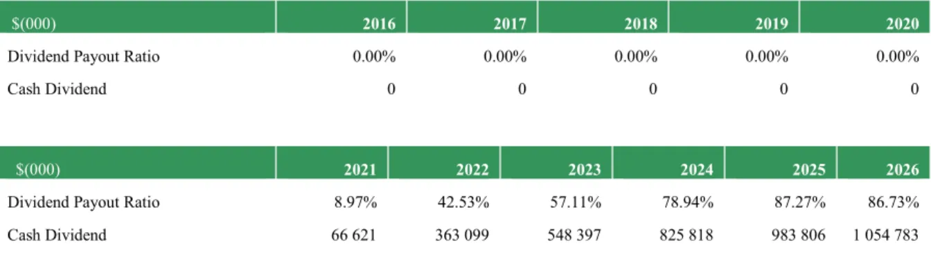
𝑀𝑜𝑑𝑖𝑓𝑖𝑒𝑑 𝑔𝑟𝑜𝑤𝑡ℎ 𝑟𝑎𝑡𝑒 = (1 – 𝑀𝑜𝑑𝑖𝑓𝑖𝑒𝑑 𝑝𝑎𝑦𝑜𝑢𝑡 𝑟𝑎𝑡𝑖𝑜) ∗ 𝑅𝑒𝑡𝑢𝑟𝑛 𝑜𝑛 𝑒𝑞𝑢𝑖𝑡𝑦 The version of the Dividend Discount Model that may be used for valuation purposes depends a lot on the fit of the company. Accounting for Under Armour Inc’s characteristics, the version that best applies is the Three Stage Dividend Discount Model.
The Three Stage Dividend Discount Model “allows for an initial period of high growth, a transitional period where growth declines and a final stable growth phase” (Damodaran, Investment Valuation, 2002). Side by side with the declining and stabilization of growth, the model assumes the maturing of the company comes with shifts in the dividend payout policy, which starts as null or very low, moves through a period of increase and ends up in the state of a high payout ratio.
The Three Stage Dividend Discount Model stands as such: 𝑆𝑡𝑜𝑐𝑘 𝑃𝑟𝑖𝑐𝑒 = ∑ 𝐸𝑃𝑆0∗ (1 + 𝑔𝑎) 𝑡∗ 𝜋 𝑎 (1 + 𝑘𝑒𝐻𝐺)𝑡 𝑡=𝑛1 𝑡=1 + ∑ 𝐷𝑃𝑆𝑡 (1 + 𝑘𝑒𝑇)𝑡 𝑡=𝑛2 𝑡=1 + ∑ 𝐸𝑃𝑆𝑛2∗ (1 + 𝑔𝑛) ∗ 𝜋𝑛 (𝑘𝑒𝑆𝑇− 𝑔𝑛) ∗ (1 + 𝑟)𝑛 𝑡=𝑛1 𝑡=1 ,
where 𝐸𝑃𝑆𝑡 equals earnings per share in year t; 𝐷𝑃𝑆𝑡 equals dividends per share in year t; 𝑔𝑎equals the growth rate in high growth phase (lasts n1 periods); 𝑔𝑛 equals growth rate in stable phase; 𝜋𝑎 equals the payout ratio in high growth phase; 𝜋𝑛 equals payout ratio in stable growth phase; 𝑘𝑒 equals required return to equity in high growth (𝐻𝐺), transition (𝑇) and stable growth (𝑆𝑇), respectively.
In this valuation, due to the lack of strong theoretical approaches to calculate the required return to equity in the transition and growth phases, it will be maintained at current levels.
A critic sometimes attributed to the DDM is that “as the market rises, fewer and fewer stocks will be found to be undervalued using the dividend discount model” (Damodaran, Investment Valuation, 2002). However, there is no evidence that DDM undervalues the stocks comparing
20
to their intrinsic value, simply that, in certain situations, it may lead to more conservative valuations than other approaches.
Concluding, the DDM will be used as a complementary model, but bearing in mind the limitations associated to the very politicized decisions of distributing dividends and the lack of strong theoretical background to forecast the future required return to equity.
2.4. Multiples/Relative Approaches
Relative Valuation’s “objective is to value assets, based upon how similar assets are currently priced in the market” (Damodaran, Investment Valuation, 2002).
There are two parts to any Relative Valuation – deciding what are the similar assets present in the market to the one we are valuing and what is the component/multiple which we are taking into consideration as a common measurement of value, both in the asset we are valuing, as in the group of similar assets.
Firstly, to solve for the latter part of the problem, one must understand the different types of measurements of value, commonly called multiples. Multiples may be divided, just as the other valuation methods, in two wide categories: enterprise multiples and equity multiples.
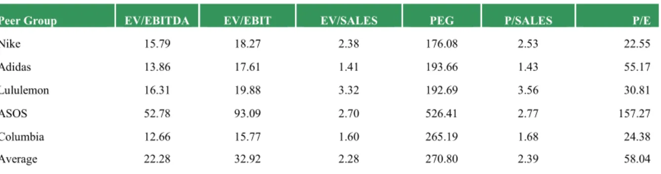
When having to decide upon which multiples to use, Foushee, Koller and Mehta (2012) claim that “most sophisticated investors and bankers compare companies relative to peers using an enterprise-value multiple – usually either EV/EBITA or EV/EBITDA. Such multiples are preferable because they are not burdened with the distortions that affect earnings ratios.” The main distortions that the authors refer are of two types. First, equity multiples tend to be affected by debt and thus will yield different values for a company with the exact same prospects, except for capital structure ratios. Second, the multiples stated are not so easy to be manipulated as if one used for example EBIT or Net income in the denominator, since these two captions already reflect some non-operating decisions of the firm. Also, by using sales instead of EBITDA, for example, we would only account for the revenue generating capacity of the assets and would disregard the operating costs that the companies incur on. For this reason, enterprise-value multiples, and specifically EV/EBITDA, will be given priority in this valuation.
One other problem in choosing the definition of multiples to use, regard timing. There are basically three different types of multiples in this sense: Current Multiples – which use accounting figures from the last financial year; Trailing Multiples – which include accounting figures from the last four quarters; Forward Multiples – based on using expected or forecasted
21
accounts for the next financial year. Goedhart, Keller and Wessels (2005) state that using forward multiples, when there are available forecasts, or at least the most recent data possible, yields much more accurate results than using Current Multiples.
Moving on to the second problem of Relative Valuation – finding comparable companies, it is known by analysts that it is impossible to find a group of firms with the exact same characteristics as the firm in question.
In the present valuation, the method chosen to control for the differences among the valued firm and the Peer Group will be a statistical tool designated cluster analysis. By taking Under Armour’s characteristics as “anchors”, or centres, the firms that are distanced the less to those characteristics will be chosen as peers. Since “every multiple… is a function of the same three variables – risk, growth and cash flow generating potential” (Damodaran, Investment Valuation, 2002), these were the characteristics in which the cluster analysis was focused, to reach the best comparable firms to value Under Armour. As a proxy for risk, the 5-year stock volatility of each firm was used, as a proxy for growth, the forecasted revenue growth rate until 2020 (Thomson Reuters forecasts) was used and as a proxy for cash flow generating potential, the trailing EBITDA margin was used.
2.5. Conclusion
After reviewing the state-of-the-art literature some decisions have been reached regarding the methods and processes that will be used in the present valuation of Under Armour Inc.
Among Enterprise Methods, Discounted Cash Flow, more specifically the Adjusted Present Value version, will play a central part in valuing Under Armour Inc. It is a possibility that the valuation reached through the Adjusted Present Value method is not the intrinsic value of the equity of the firm in question, since the method to calculate Costs of Financial Distress and Present Value of Interest Tax Shields still does not generate consensus. However, it should be closer to it than if WACC was to be used, considering this method does not even account for the effects of financing side effects other than tax shields, and even tax shields are included in a very opaque way. The Economic Value Added approach will be left out, mainly due to the problems usually associated to it – the difficulty in finding a good proxy for the Capital Invested and the high dependency of this model on the Weighted Average Cost of Capital, that we left out due to its limitations.
22
Among Equity Methods, the Dividend Discount Model will be used, as another component that shall add consistency to this valuation, and due to its conservative character, which should help defining a lower bound for the valuation. The specific version of the DDM which will be used is the Three Stage Dividend Discount Model.
Lastly, a Relative Valuation will be put to practice, using a cluster analysis, to control for differences in comparable companies and giving priority to enterprise multiples, EV/EBITDA more than any other.
23 3. Company Overview
Under Armour Inc is an American born firm operating in the Global Sportswear Industry. The company was created in 1996, by the then Football Special Teams Captain of the University of Maryland – Kevin Plank. In that year, UA targeted the lack of performance-driven football shirts available, with the creation of the first product of the kind by the founder, designated by “Prototype 0037”, which was soft, tight and able to wick sweat in a better way than any existing products.
Innovativeness stands at the core of the company’s mission – “to make all athletes better through passion, design and the relentless pursuit of innovation”, and this characteristic is still presently associated to the company, which stands at number 6 in the Forbes 2016 “The World’s Most Innovative Companies” ranking.
On November 18, 2005 Under Armour’s IPO took place. The company’s underpricing was a record one, with UA becoming the first United States based IPO to double on its first day of tradingin the five years prior to that date, opening at 31$ per share against the original price of 13$ per share. The offering’s underwriting group, Goldman Sachs, valued the equity of the company at 157,3 million dollars.
The huge growth of the company, however, would not stop at that point. In the period between the Initial Public Offering and 2010, UA almost quadruplicated its revenues, surpassing $1 billion in annual revenues.
At the present date, Under Armour defines its activities as developing, marketing and distributing of their branded performance apparel products and is ranked 6th in the world in the global sportswear industry revenue-wise and totalizes a market capitalization of over $16.5 Billion. The company presently enjoys three revenue sources – sportswear sales, licensing revenues and Connected Fitness revenues, which are revenues derived from an investment made by Under Armour in a mobile app as well as devices that are connected to such app and make it possible for users to save and share their fitness performance with each other.
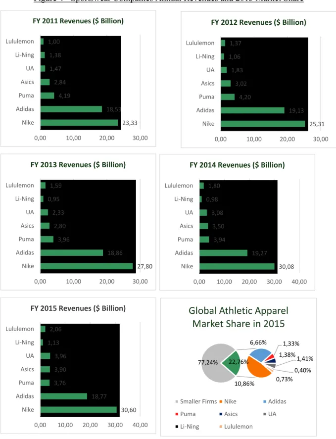
By enjoying a 5-year compound net revenues growth rate of 30.1%, Under Armour is currently competing head-to-head for global athletic apparel market share, against companies with extremely large size, strong financial resources, and very well established brands.
24 4. Industry Overview
4.1. Macro Analysis
Sportswear, comprised of sports apparel and footwear is an industry that has been experiencing exponential growth in the recent past. The worldwide market was estimated to have grown at a CAGR of 6% (Societe Generale, 2016) since 2010, adding up to $281,9 bn in 2015. The main macro tailwinds that the industry has been exposed to were the increase in the participation of sports by youth, and mainly the general increase in awareness for health and the necessity to exercise. Consumption by continent in $ bilion stands as follows:
Figure 1 - Sportswear Consumption by Region, 2015 ($bn)
Source: Societe Generale "Global Sportswear Industry: Steadily Growing but Fragmented"
North America continues to lead the global consumption, almost doubling the registered figures from Western Europe and Asia. In gender terms, the market is still dominated by men but it has been showing a trend of gender uniformisation, with the women segment gaining ground due to social tailwinds, after being neglected for a long time.
102 24,9 58,1 15,3 16,8 64,8
North America South America Western Europe Eastern Europe Middle East and Africa Asia
25
Figure 2 - Sportswear Industry Consumer by Gender
Source: Societe Generale "Global Sportswear Industry:Steadily Growing But Fragmented"
The recent overall growth experienced by the industry is expected to continue in the future. Societe Generale’s estimates place growth expectations at a CAGR of 5,3%, implying possible sales values of $365 bn by 2020.
This growth is dependent on a variety of macro factors that affect this industry. First, major sporting events such as the Uefa Euro 2016 and Rio 2016 Olympic Games are expected to boost the annual 2016 sales figures. Wage increases are expected both in developed countries as well as emerging ones. Private consumption is expected to grow benefiting from the increase in disposable income. However, at the same time, production costs are expected to rise as a direct effect of the wage improvement in the areas where companies manufacture goods, in general. One specific area of the industry which should continue to gain traction is e-commerce, with firms expected to increase digital spending even further.
Positive social factors are also expected to be maintained, as health consciousness and trends regarding social fitness are expected to grow even further. This trend should help the women segment to grow strongly. Maintained investment in the children segment in the shape of incentives to participation in sports and encouragement to have healthier lifestyles are expected to continue helping this segment’s growth as well.
Industry consumption annual growth rates vary depending on the region:
52% 35%
13%
26
Graph 1 - Industry Regional Average Annual Growth
Source: Societe Generale "Global Sportswear Industry: Steadily Growing but Fragmented"
North America and EMEA are both expected to enjoy an increase in growth rates due to the economic and social factors already addressed. On the other side, Latin America should lose some acceleration, as the deep recessions felt in Brazil and Argentina, political instability and high inflation across the region are expected to play an important part in the industry’s development. Forecasts point at Asia as having the biggest percentage increase in growth in the next five years, also benefiting from strong industrial activities, increases in wage levels and low oil prices.
4.2. Micro Analysis
To assess the current attractiveness of the global athletic apparel industry, one may use the Porter’s 5 Forces model.
Firstly, product differentiation within the industry is limited, in general terms, with the same materials (such as fabrics) and main technologies being available to a majority, if not all, of firms. Together with rapid product cycles and the existence of relatively high economies of scale, the threat of new entry is weak.
On the other hand, the high similarity of products used between firms, the very low cost of switching costs and the importance of some retailer customers make the customer bargaining power to be moderately strong.
6,30% 4,00% 6,30% 10,50% 6,70% 4,40% 8,50% 6,10% 0,00% 2,00% 4,00% 6,00% 8,00% 10,00% 12,00%
North America EMEA Asia Latin America
27
In terms of product substitution, the low switching costs are more than offset by the low availability of high performance product substitutes, turning the threat of substitute products in a moderately weak one.
Regarding the bargaining power of suppliers, mostly raw materials, the low number of firms supplying high quality raw materials and the increasing demand for these raw materials turns this force into a moderately strong one.
Finally, the competitive rivalry is considered a strong one. Although the high number of firms weakens the effect, the bi-modal character of the industry (has a group of very large global firms dominating demand, and a high number of much smaller firms competing for niche markets and local demand), the high maturity of the industry, also associated to a low average growth rate, rapid changes in consumer preferences and product cycles, and the difficulty to get fabric or process patents have a very strong effect in increasing competition. The Porter’s 5 Forces model will stand as follows:
Source: Own Analysis
The similarity of production costs among the largest firms, together with the relatively high product similarity have two very important effects in the industry dynamics. The first one is the enormous competition for retailer space, that pressures prices of those businesses down.
Competitive Rivalry Threat of Substitutes Threat of New Entries Bargaining Power of Suppliers Bargaining Power of Customers Weak Moderately Weak Moderately Strong Strong
28
The second effect, and even a more important one, is each firm’s necessity to distinguish itself from competition. One of the direct consequences of this necessity is the incredibly high marketing costs incurred by each of the larger firms in business, with the tendency to have promotion, advertising and demand creation expenses adding up to more than 10% of gross revenues, for larger firms.
Other consequences are the constant increase in the pace of product development and introduction and a growing number of trademarks and patents that each firm claims. Trademarks in this industry are sometimes considered one of the most valuable assets owned by firms due to the differentiating power they confer.
One last, but very important factor in the industry is the quality of human capital. Since the market requires an enormous deal of innovativeness in product development, marketing and brand strengthening, strong leadership and highly qualified personnel are key to the success in this market.
29 5. Valuation Inputs– APV
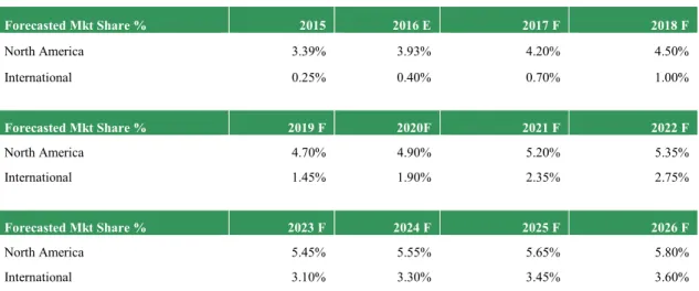
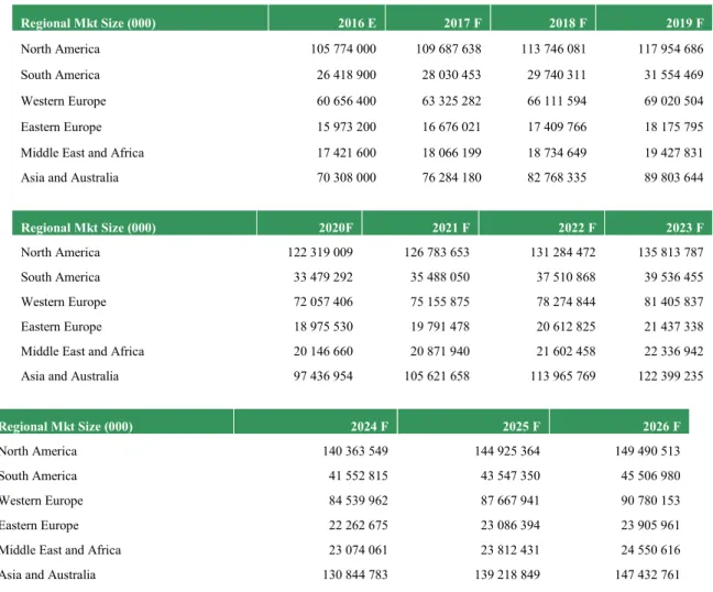
The present valuation relied in a group of factors to forecast Under Armour’s operations. One of them, and already presented in the Macro Analysis, is the growth of the Global Sportswear Industry and the demand for such products, in this case given by Societe Generale’s research. The given growth combined with the evolution of Under Armour’s market share shall combine and reflect the company’s operations scale in future years.
By putting this factors in perspective, together with the company’s expectations on the evolution of its own operations and the potential of other industry players, the final result should be a well-informed valuation, supported by the most reliable and concrete data possible.
5.1. Revenue estimation
In the 2015 FY, Under Armour ended up reporting $3.96 bn in revenue, experiencing a yoy revenue growth of approximately 28.5% and capturing a market share of 3.39% in North America and 0.25% globally (excluding North America).
UA’s future revenue growth used in this valuation model stands as such: Table 1 - UA Revenue Segmentation by Region
Revenue by region ($ Thousands) 2011 2012 2013 2014 2015
North America 1 383 346 1 726 733 2 193 739 2 796 374 3 455 737 International 89 338 108 188 137 244 268 771 454 161
Connected Fitness - Global 0 0 1 068 19 225 53 415
Total Net revenues 1 472 684 1 834 921 2 332 051 3 084 370 3 963 313
Source: Own Analysis and Company Reports
Table 2- UA Revenue Forecast
Revenue Forecast ($ 000) 2016 E 2017 F 2018 F 2019 F 2020 F
North America 4 153 796 4 606 881 5 118 574 5 543 870 5 993 631 International 4 910 428 6 023 556 7 266 220 8 849 613 10 593 452 Connected Fitness - Global 91 179 136 769 202 418 297 555 384 980 Global Net Revenues 5 001 608 6 160 325 7 468 638 9 147 168 10 978 432
30
Revenue Forecast ($ 000) 2021 F 2022 F 2023 F 2024 F 2025 F 2026 F
North America 6 592 750 7 023 719 7 401 851 7 790 177 8 188 283 8 670 450 International 12 630 581 14 502 805 16 302 441 17 765 229 19 136 270 20 628 803 Connected Fitness - Global 443 333 509 048 572 216 623 560 671 683 724 071 Global Net Revenues 13 073 915 15 011 854 16 874 657 18 388 788 19 807 953 21 352 874
Source: Own Analysis and Company Reports
The forecast of future revenues in this model was anchored in three main factors. The first one was expected industry growth, based both on Societe Generale’s forecasts and author inputs. The second one was the market share evolution for Under Armour. The third one was the company’s own forecasts, which set revenue expectations for 2018 at slightly under $7.5 bn (in line with this model) and revenue growth at between 20 and 25%, for next few years.
The figures above are linked to the following revenue growth and market share, in each year: Table 3 - UA Revenue and Market Share Evolution
Year Revenue Growth Rate N. America Mkt Share Int. Market share
2016 26.20% 3.93% 0.40% 2017 23.17% 4.20% 0.70% 2018 21.24% 4.50% 1.00% 2019 22.47% 4.70% 1.45% 2020 20.02% 4.90% 1.90% 2021 19.09% 5.20% 2.35% 2022 14.82% 5.35% 2.75% 2023 12.41% 5.45% 3.10% 2024 8.97% 5.55% 3.30% 2025 7.72% 5.65% 3.45% 2026 7.80% 5.80% 3.60%
Source: Own Analysis and Company Reports
Independent forecasts made by Thomson Reuters and FactSet place revenue forecasts for Under Armour very close to the figures shown in this model, which further demonstrates the high likelihood of this scenario.
5.2. Cost of Goods Sold / Gross Margin
For a retail company, such as the one currently in discussion, gross margin assumes an essential figure in determining the success of a firm.
31
Table 4 - UA COGS and Growth Margin Forecast
2011 2012 2013 2014 2015 2016 E 2017 F 2018 F COGS 759 848 955 624 1 195 381 1 572 164 2 057 766 2 645 850 3 258 812 3 950 910 Gross Margin 48.40% 47.92% 48.74% 49.03% 48.08% 47.10% 47.10% 47.10% 2019 F 2020 F 2021 F 2022 F 2023 F 2024 F 2025 F 2026 F COGS 4 838 852 5 807 591 6 916 101 7 941 271 8 926 694 9 727 669 10 478 407 11 295 670 Gross Margin 47.10% 47.10% 47.10% 47.10% 47.10% 47.10% 47.10% 47.10%
Source: Own Analysis and Company Reports
At a first glance, it might seem out of context to forecast the future gross margin at a value lower than recent past ones. However, despite registering an average gross margin of 48.43% for the last 5 fiscal years, Under Armour has seen its third quarter 2015 gross margin lowered to 47.3%. The factors presented in the micro analysis such as increased competition for retailer space may pressure prices down even more, hence the low margin forecast.
The recent drop in share price registered by the company is closely linked to this “margin crushing”, as well as to the lower revenue growth expectations, both referred in the 2015 Investor Day. Thomson Reuters estimates also place gross margins at lower than historical values – average of 47.5% between 2016 and 2020. This model will use a slightly more conservative approach of maintaining the figure at 47.1% in future.
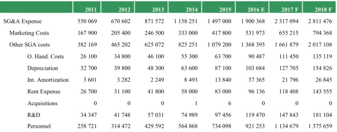
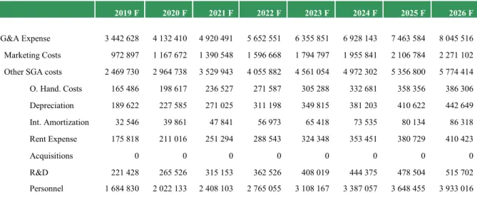
5.3. Selling, General and Administrative Expense
This caption in the company’s statement of income comprises all operating expenses other than costs of goods sold. The evolution of these costs stands as such:
Table 5 - UA Historical and Forecasted SG&A
2011 2012 2013 2014 2015 2016 E 2017 F 2018 F
SG&A Expense 550 069 670 602 871 572 1 158 251 1 497 000 1 900 368 2 317 094 2 811 476 Marketing Costs 167 900 205 400 246 500 333 000 417 800 531 973 655 215 794 368 Other SGA costs 382 169 465 202 625 072 825 251 1 079 200 1 368 395 1 661 879 2 017 108 O. Hand. Costs 26 100 34 800 46 100 55 300 63 700 90 487 111 450 135 119 Depreciation 32 700 39 800 48 300 63 600 87 100 103 684 127 705 154 826 Int. Amortization 3 601 3 282 2 249 8 493 13 840 37 365 21 796 26 845 Rent Expense 26 700 31 100 41 800 58 000 83 000 96 136 118 408 143 555 Acquisitions 0 0 0 1 6 0 0 0 R&D 34 347 41 748 57 031 74 989 97 456 119 470 147 843 181 104 Personnel 258 721 314 472 429 592 564 868 734 098 921 253 1 134 679 1 375 659
32
2019 F 2020 F 2021 F 2022 F 2023 F 2024 F 2025 F 2026 F
SG&A Expense 3 442 628 4 132 410 4 920 491 5 652 551 6 355 851 6 928 143 7 463 584 8 045 516 Marketing Costs 972 897 1 167 672 1 390 548 1 596 668 1 794 797 1 955 841 2 106 784 2 271 102 Other SGA costs 2 469 730 2 964 738 3 529 943 4 055 882 4 561 054 4 972 302 5 356 800 5 774 414 O. Hand. Costs 165 486 198 617 236 527 271 587 305 288 332 681 358 356 386 306 Depreciation 189 622 227 585 271 025 311 198 349 815 381 203 410 622 442 649 Int. Amortization 32 546 39 861 47 841 56 973 65 418 73 535 80 134 86 318 Rent Expense 175 818 211 016 251 294 288 543 324 348 353 451 380 729 410 423 Acquisitions 0 0 0 0 0 0 0 0 R&D 221 428 265 526 315 153 362 526 408 019 444 375 478 504 515 702 Personnel 1 684 830 2 022 133 2 408 103 2 765 055 3 108 167 3 387 057 3 648 455 3 933 016
Source: Own Analysis and Company Reports
The basis for each caption forecasts stands below:
Table 6 – UA SG&A Expenses Inputs
2011 2012 2013 2014 2015 2016 E 2017 F 2018 F
Marketing / Revenues 11.40% 11.19% 10.57% 10.80% 10.54% 10.64% 10.64% 10.64% O. Handling Costs / Revenues 1.77% 1.90% 1.98% 1.79% 1.61% 1.81% 1.81% 1.81% Depreciation / gross PPE 11.94% 12.20% 12.19% 12.18% 10.47% 11.80% 11.80% 11.80% Intangible Amort. / LY Intangibles -- 59.30% 50.17% 35.25% 52.76% 49.37% 49.37% 49.37% Rent Expense / Op. Leases 14.42% 15.33% 12.90% 12.27% 13.25% 12.81% 12.81% 12.81% R&D Expenses / Revenues 2.33% 2.28% 2.45% 2.43% 2.46% 2.39% 2.39% 2.39% Personnel Costs / Revenues 17.57% 17.14% 18.42% 18.31% 18.52% 18.42% 18.42% 18.42%
2019 F 2020 F 2021 F 2022 F 2023 F 2024 F 2025 F 2026 F
Marketing / Revenues 10.64% 10.64% 10.64% 10.64% 10.64% 10.64% 10.64% 10.64% O. Handling Costs / Revenues 1.81% 1.81% 1.81% 1.81% 1.81% 1.81% 1.81% 1.81% Depreciation / gross PPE 11.80% 11.80% 11.80% 11.80% 11.80% 11.80% 11.80% 11.80% Intangible Amort. / LY Intangibles 49.37% 49.37% 49.37% 49.37% 49.37% 49.37% 49.37% 49.37% Rent Expense / Op. Leases 12.81% 12.81% 12.81% 12.81% 12.81% 12.81% 12.81% 12.81% R&D Expenses / Revenues 2.39% 2.39% 2.39% 2.39% 2.39% 2.39% 2.39% 2.39% Personnel Costs / Revenues 18.42% 18.42% 18.42% 18.42% 18.42% 18.42% 18.42% 18.42%
Source: Own Analysis and Company Reports
Marketing expenses tend to have major weight in sportswear companies and in this model’s case, these expenses are forecasted to grow at 10.64% of revenues. This value is reached
33
through the average of the last 3 fiscal years’ ratios, and not the last 5 years, since Under Armour registered a decrease in these costs since 2013, comparing to the two periods before that one. Outbound handling costs are costs related to materials used in shipping products, and they are forecasted to be maintained, on average and as a percentage of revenues, relatively to the last 5 years.
Depreciation is forecasted through a percentage of gross power, plant and equipment. This percentage is 11.8%, which corresponds to the last 5-year average.
Intangible amortization is expected to remain at 49.37% of the previous year’s intangibles, also according to its past average.
Rent expense for Under Armour represents the expenses related to lease payments and they will be forecasted at 12.81% of operating leases outstanding in each year. This percentage was reached through an average of the last 3 years, since the company lowered this expenses, comparing to 2011 and 2012, in percentage.
Research and development expenses are set, in the model at 2.39% of revenues, with this being the average percentage value for the past 5 years, for UA.
Lastly, personnel costs are forecasted at 18.42% of net revenues. This value was reached through the average of the last 3 years. The reason for the choice of the 3-year period was the increase in this type of costs felt by Under Armour, comparing to 2011 and 2012. This inflated personnel costs may be related to the macro economic factors explained in a previous sector and those factors are expected to be maintained, if not increased.
5.4. Debt Outstanding and Interest Expense
For the time being, Under Armour has some public debt outstanding – since the issuance of $600m worth of bonds in the beginning of June, 2016. Besides this type, the company still has some debt outstanding derived from a revolving credit facility, besides a high value outstanding for operating leases.
The full inputs and forecast for the debt outstanding may be consulted in the Appendix 7 -Debt Forecast Inputs.
5.5. Other expense
The other expense rubric comprises, for Under Armour, income mainly related to derivatives and foreign currency exchange rate contracts, used for hedging.
34
Since hedging may be considered an activity directly linked to the operations level of the company, these expenses were forecasted to grow with operations, at 0.12% of the net revenues – the past 5-year historic average.
5.6. Effective tax-rate
During the period analysed (2011-2015), the company’s effective tax rate has been maintained at relatively stable levels (between 36.7% and 39.85%). With that said, this rate is forecasted to be maintained at 38.36% in the future, an average of the past 5 years.
5.7. Working Capital
The generic method to forecast future working capital requirements was through a past analysis of the Days of Sales Outstanding (DSO), Days Payable Outstanding (DPO) and Days of Inventory Held (DIH).
The ratios were maintained at an average of the past 5-year period, with three exceptions: accounts receivable, accounts payable and deferred income taxes. Since Under Armour has seen a gradual change in working capital requirements, the DSO related to accounts receivable have increased and the DPO related to accounts payable have decreased, up to the present. Since using an average may provide biases, the DPO and DSO values witnessed in 2015 were maintained in the future.
Deferred income taxes-current assets are stated at zero in 2015 and in all the years after that. The reason for that is an accounting standards update issued by the FASB, requiring deferred tax assets and liabilities to be reclassified as non-current on the balance sheet. This amendment was applied prospectively by Under Armour.
5.8. Capitalizing R&D
R&D expenses are capitalized in our model in an off-balance sheet method. According to such method, R&D expense in each period is added to the capital expenditures (otherwise only comprised of the purchases in property, plant and equipment), and amortized through time. The R&D amortizable life period used was 2 years – period used for special retail lines.
In the capitalization process, adjusted operating income after tax (NOPAT), capex and depreciations and amortizations values were reached.