ABSTRACT: Vegetation indices are widely used to monitor crop development and generally used as input data in models to forecast yield. The first step of this study consisted of using monthly Maximum Value Composites to create correlation maps using Enhanced Vegetation Index (EVI) from Moderate Resolution Imaging Spectroradiometer (MODIS) sensor mounted on Terra satellite and historical yield during the soybean crop cycle in Paraná State, Brazil, from 2000/2001 to 2010/2011. We compared the ability of forecasting crop yield based on correlation maps and crop specific masks. We ran a preliminary regression model to test its ability on yield estimation for four municipalities during the soybean growing season. A regression model was developed for both methodologies to forecast soybean crop yield using leave-one-out cross validation. The Root Mean Squared Error (RMSE) values in the implementation of the model ranged from 0.037 t ha−1 to 0.19 t ha−1 using correlation maps, while for crop specific masks, it varied from 0.21 t ha−1 to 0.35 t ha−1. The model was able to explain 96 % to 98 % of the variance in esti-mated yield from correlation maps, while it was able to explain only 2 % to 67 % for crop specific mask approach. The results showed that the correlation maps could be used to predict crop yield more effectively than crop specific masks. In addition, this method can provide an indication of soybean yield prior to harvesting.
Keywords: MODIS, crop yield forecasting, vegetation indices 1University of Campinas/FEAGRI, Av. Cândido Rondon, 501 −
13083-875 − Campinas, SP − Brazil.
2University of Kansas − Dept. Of Geography, 1475 Jayhawk Blvd − 66045 − Lawrence, KS − USA.
3University of Campinas/NIPE, R. Cora Coralina, 330, C.P. 6166 − 13083-896 − Campinas, SP − Brazil.
*Corresponding author <[email protected]>
Edited by: Dionysis Bochtis
Correlation maps to assess soybean yield from EVI data in Paraná State, Brazil
Gleyce Kelly Dantas Araújo Figueiredo1*, Nathaniel Allan Brunsell2, Breno Hiroyuki Higa1, Jansle Vieira Rocha1, Rubens Augusto Camargo Lamparelli3
Received May 13, 2015 Accepted November 05, 2015
Introduction
Monitoring agricultural crops during the growing season is important to forecast yield prior to harvesting (González-Sanpedro et al., 2008). Several techniques have been developed to achieve accurate yield estimates, namely the linear regression analysis based on remote sensing data (Wall et al., 2008). This approach is based on estimating photosynthetic capacity from vegetation indices related to yield (Becker-Reshef et al., 2010).
The Moderate Resolution Imaging Spectroradiometer (MODIS) data have great potential to monitor biophysical parameters (Huete et al., 2002) and improve accuracy in crop yield assessment (Ren et al., 2008; Funk and Budde, 2009). The coarse spatial resolution is a limiting factor to the use of MODIS data, which results in mixed pixels that may not be suitable for crop yield models (Shao et al., 2015).
Several approaches have been tried to address this problem. Genovese et al. (2001) applied weighted Normalized Vegetation Index (NDVI), called CORINE-NDVI (CCORINE-NDVI) to extract indicators for crop yield monitoring in Spain. The authors found that indicators based on CNDVI were more closely related to crop yield than those based on NDVI. Becker-Reshef et al. (2010) used a regression model to estimate wheat yield in Kansas, the United States, based on a percentage map using the pure pixels that allowed reliable yield estimates prior to harvesting.
Maselli and Rembold (2001) found that improvement in estimates of yield capacity depends on the crop and the values of vegetation index considered in the area. The authors estimated yield in North
African countries by correlating NDVI and yield. They reported that areas with low NDVI values could present high correlation due to the presence of grasses with a similar phenology, such as cereals. Combining both the percentage map and the correlation between NDVI and yield, Kastens et al. (2005) created the "yield-correlation masking" approach to estimate cereal yield in the United States. The authors found that vegetation in a region can integrate the growing conditions, which could be more indicative of crop potential.
Several studies in Brazil have achieved reliable results using the regression analysis to estimate yield (e.g. Gusso et al., 2013; Picoli et al., 2014), however, the crop mask of these methods does not always represent the reality of the area. Therefore, this study investigates the potential of using correlation maps to estimate soybean yield based on the regression analysis and find the suitable period to estimate yield in Brazil.
Materials and Methods
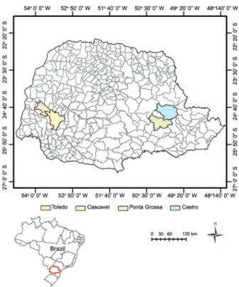
According to the Köppen's climate classification map for Brazil (Alvarez et al., 2013), the climate in Paraná state is Cfa type (i.e., subtropical mesothermal climate) and Cfb type (i.e., temperate mesothermal cli-mate). The average annual temperatures is 19 °C, with the hottest month averaging above 22 °C and the coldest below 18 °C.
Agricultural statistics for the soybean growing sea-son were collected from the Department of Agriculture and Supply of Paraná (SEAB) database and the Brazilian Institute of Geography and Statistics (IBGE). Both SEAB and IBGE obtain data through agricultural surveys with growers and cooperatives. These data were used to cre-ate a time series of soybean area and total production for the period between 2000/2001 and 2010/2011 growing seasons. Table 1 shows statistics for the soybean area and yield time series used in this study.
Enhanced Vegetation Index (EVI) images were ob-tained from Moderate Resolution Imaging Spectroradi-ometer (MODIS) mounted on Terra satellite that is part of Earth Observing System (EOS) program. MODIS/Terra views the entire Earth's surface every one to two days. It has sun-synchronous orbit at 705 km and crosses the equator line at 10:30 a.m. descending node. The MODIS data provide high radiometric sensitivity (12 bits) in 36 spectral bands ranging at wavelength from 0.4 µm to 14.4 µm (Nasa, 2013a).
The images were obtained from Brazilian State Base, a dataset held by the Brazilian Agricultural Research Corporation, Agricultural Informatics (Embrapa Infor-mática Agropecuária), which provides images derived from MOD13Q1 product (Embrapa, 2011). MOD13Q1 data are provided by the LPDAAC/EOS (Land Processes Distributed Active Archive Center/NASAs Earth Observ-ing System) every 16 days at 250-meter spatial resolution as a gridded level-3 product in the Sinusoidal projection (Nasa, 2013b).
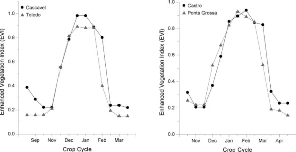
Soybean crop is cultivated during the summer season in Brazil. For the study region, the planting date occurs approximately between October and December, which corresponds to the period of high rainfall, while the harvesting period occurs from February to April
(Ta-Table 1 − Planted area and historical yield for the study area from 2000/2001 to 2010/2011 crop seasons.
Crop Season
Soybean area (ha)
Yield (t ha−1)
Soybean area (ha)
Yield (t ha−1)
Soybean area (ha)
Yield (t ha−1)
Soybean area (ha)
Yield (t ha−1)
Cascavel Toledo Castro Ponta Grossa
2000/2001 72100 2.50 64000 2.85 47000 3.00 41000 2.95
2001/2002 67652 3.18 62900 3.46 46000 3.20 40000 3.20
2002/2003 74689 2.89 66100 3.23 60000 3.15 48000 3.10
2003/2004 78200 3.31 67150 3.47 64000 3.40 55000 3.38
2004/2005 83000 2.73 68850 2.40 65200 3.10 57050 3.30
2005/2006 87700 2.36 69300 2.72 70000 3.15 65000 3.15
2006/2007 83700 2.68 66900 2.22 65000 3.00 59000 2.76
2007/2008 84000 2.84 66100 3.12 67000 3.30 60100 3.20
2008/2009 82850 3.24 65300 3.16 72300 3.13 63000 3.20
2009/2010 84000 2.55 64100 2.26 79000 2.58 65350 2.70
2010/2011 89800 3.32 67802 3.40 79800 3.25 68300 3.20
Mean 81149.25 2.92 66208.50 2.97 66316.67 3.15 57675.00 3.14
SD 6362.87 0.35 1861.91 0.45 10908.01 0.22 9628.29 0.22
CV 0.08 0.12 0.03 0.15 0.16 0.07 0.17 0.07
Trend 72673.12 2.73 65588.92 3.00 50016.67 3.13 43413.46 3.11
Area (km²) 2,100,831 1,196,999 2,531,503 2,067,547
ble 2). Figure 2 shows the average soybean crop cycle for the study region. Acquisition of cloud-free images was al-most impossible, therefore, the monthly Maximum Value Composite (MVC) imagery was used.
Correlation Maps
There are many methodologies to establish a rela-tionship between vegetation indices and final yield. The methods are often based on monthly vegetation indices values (Maselli and Rembold, 2001) or on accumulation over determined periods of the crop phenological stage (Tucker et al., 1980; Rasmussen, 1992; Genovese et al., 2001; Kastens et al., 2005; Ren et al., 2008).
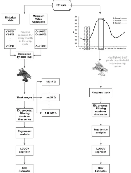
To examine variation in correlation with crop de-velopment, this study was based on the first approach in which the monthly EVI values were regressed with the historical soybean yield values at the pixel level. The first step examined each month separately, for example, the 11 images from October were arranged and regressed with the annual yield values. This process was repeated for
ev-ery month of the growing season. Thus, the correlation maps were built based on the crop cycle of each munici-pality.
Regression model
The correlation maps were used to build masks with different correlation ranges to assess the ability of each range to estimate yield. Kastens et al. (2005) used a similar approach by applying masks with different sizes to test its capacity to forecast yield.
In this study, the ranges were separated as the correlation increased. Therefore, the first mask corre-sponds to the range 0-10 % of correlation, the second 11-20 %, and this process was repeated until a correla-tion of 100 %.
For comparison purposes, we used crop specific masks to estimate yield and compared it with the meth-odology proposed here. For these crop specific masks, we followed the methodology described by Araújo et al. (2011), where multi-temporal color composites were cre-ated in RGB channels. The color composites were based on the soybean crop cycle in which the Red channel corresponds to the vegetative peak, and the Green and Blue channels correspond to the beginning of the crop cycle, thus, only the soybean crop was highlighted in the composite. This process was repeated until the end of the phenological cycle due to differences in the planting dates in the state. A color composite was generated for each 16-day period.
In order to create a soybean specific crop layer, pix-els from the composites described above were selected with gray level values above 200 on the Red channel and below 200 on the Green and Blue channels. This resulted in a binary classification of the soybean areas. To gener-ate the final annual soybean classification, the 16-day soy-bean masks were overlapped for the entire study area.
Table 2 − Monthly percentage of planting and harvesting soybean crop season in Paraná State*.
Planting period Harvesting period
Crop Season Oct Nov Dec Jan Feb Mar Apr May
%
---2004/2005 20 73 6 - 16 50 27 7
2005/2006 37 58 5 1 8 55 31 5
2006/2007 23 66 11 - 13 54 29 4
2007/2008 23 63 14 - 11 45 34 10
2008/2009 24 58 18 - 1 50 41 8
2009/2010 50 47 3 1 16 58 21 4
2010/2011 47 51 2 - 5 80 13 2
*Data from 2000/2001 until 2003/2004 was not provided. Source: SEAB/ Deral (2013).
This process was applied to generate a soybean crop mask for each year of study. Figure 3 illustrates the main steps of the study.
An automated process was applied to extract pixels from the time-series data based on the masks. We used the system developed by Esquerdo et al. (2011). This sys-tem requires the time-series and the coordinate location of the fields (extracted from the masks), which results in the EVI values corresponding to the masks. Then, these pixels were used as input data to estimate yield. A similar approach was used by (Fernandes et al., 2011).
For each of the correlation masks and approaches of crop specific masks to quantify yield, a linear regres-sion model (equation 1) was developed to calculate the estimated yield:
Y = a + b×EVI (1)
where Y is the estimated soybean yield; EVI is from the
monthly MVC composite; a and b are the regression
equa-tion parameters.
The residual analysis was applied to verify ho-moscedasticity, normality and independence of residuals (Breusch and Pagan, 1979; Shapiro and Wilk, 1965). In ad-dition, the absence of autocorrelation in the data was veri-fied. As a final test, we developed regression models using a “leave-one-out” cross validation to validate the estimat-ed yield. All error values were calculatestimat-ed by comparing the observed and estimated yield. The fraction of soybean yield variation, which was explained by the progressive addition of EVI in the linear regression analysis, was quantified by means of the coefficient of determination (R²). The Root Mean Squared Error (RMSE) was used to measure the model performance and the Mean Absolute Error (MAE) was used to measure the model accuracy. Furthermore, the Willmott index of agreement (d) (Will-mott, 1981) was used to measure the degree of accuracy between estimated and observed values.
Results and Discussion
Correlation Maps
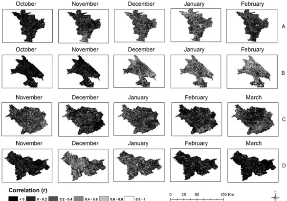
Figure 4 shows which period had the strongest correlation between EVI and historical yield. The low correlation for Oct and Nov indicated that EVI during this period did not result in a good correlation with yield data. This period corresponded to the beginning of the crop cycle, thus, pixels consist of a spectral mixture of both plant and soil.
In Cascavel and Toledo, the highest correlation between EVI and yield occured in Dec, Jan and Feb, while in Ponta Grossa, Dec and Jan showed the highest values. This can be explained because this period corresponds to the vegetative peak of the crop cycle and, consequently, high EVI values. Correlation maps for Castro were not able to detect periods with high correlation, since this municipality does not consist of large soybean crops, as observed in the other regions.
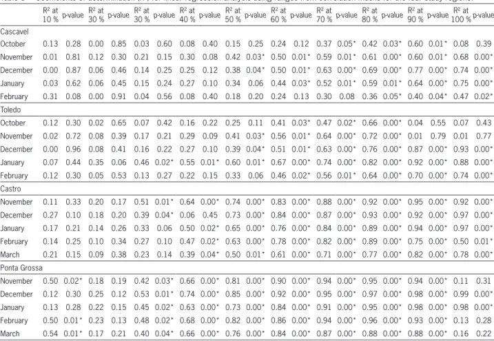
Table 3 presents the coefficient of determination (R²) for the linear regression analyses using the ranges from the correlation masks. As the correlation range in-creases, R² becomes stronger and, thus, the significance level is improved. Analyzing the crop growth, we confirm that the highest values of R² occurred during Dec, with Oct and Nov having the lowest predictive capacity for annual yield estimates. December, Jan and Feb approxi-mately corresponded to the flowering and filling seed phe-nological stages in Cascavel and Toledo. In Ponta Grossa, Feb presented the highest correlations (R² < 0.5).
Evaluating each range of correlation mask, we found that a good coefficient of determination was reached at 0.60 for the western region. On the other hand, for the eastern region, ranges between 0.50 and 0.40 for Castro and Ponta Grossa, respectively, pre-sented good results and for both regions, R² improved as the range increased achieving the highest values at 1.00. This is linked to soil and climate differences of both regions, where the western region is located in the humid subtropical climate with an annual average rainfall between 1800 mm and 2000 mm, Oxisol soil type and elevation between 600-750 m. The eastern region has temperate climate, annual average rainfall between 1600 mm and 1800 mm, inceptsol soils and elevation between 900-1100 meters (IAPAR, 2013; USDA, 2005).
Maselli and Rembold (2001) and Kastens et al. (2005) reported that the correlation map could perform well in regions of sparse crop distribution, such as in the eastern region of our study area, once it can express information on the fractional land cover in a pixel. Our analysis supports the general findings of these previous studies.
Estimated yield: correlation maps versus crop spe-cific masks
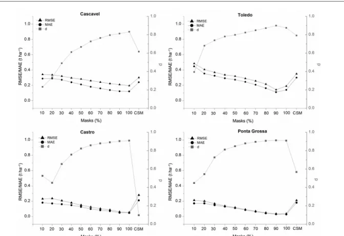
The performance of all correlation masks and crop specific mask is shown in Figure 5. The approach of crop specific mask for the four municipalities studied showed low performance, however, it was lower in
Table 3 − Coefficients of determination (R²) for linear regression analysis using ranges from correlation masks for the four study regions. R² at
10 % p-value R² at 30 % p-value
R² at 30 % p-value
R² at 40 % p-value
R² at 50 % p-value
R² at 60 % p-value
R² at 70 % p-value
R² at 80 % p-value
R² at 90 % p-value
R² at 100 %p-value Cascavel
October 0.13 0.28 0.00 0.85 0.03 0.60 0.08 0.40 0.15 0.25 0.24 0.12 0.37 0.05* 0.42 0.03* 0.60 0.01* 0.08 0.39 November 0.01 0.81 0.12 0.30 0.21 0.15 0.30 0.08 0.42 0.03* 0.50 0.01* 0.59 0.01* 0.61 0.00* 0.60 0.01* 0.68 0.00* December 0.00 0.87 0.06 0.46 0.14 0.25 0.25 0.12 0.38 0.04* 0.50 0.01* 0.63 0.00* 0.69 0.00* 0.77 0.00* 0.74 0.00* January 0.03 0.62 0.06 0.45 0.15 0.24 0.27 0.10 0.34 0.06 0.44 0.03* 0.52 0.01* 0.59 0.01* 0.64 0.00* 0.75 0.00* February 0.31 0.08 0.00 0.91 0.04 0.56 0.08 0.40 0.18 0.20 0.24 0.13 0.30 0.08 0.36 0.05* 0.40 0.04* 0.47 0.02* Toledo
October 0.12 0.30 0.02 0.65 0.07 0.42 0.16 0.22 0.25 0.11 0.41 0.03* 0.47 0.02* 0.66 0.00* 0.04 0.55 0.07 0.43 November 0.02 0.72 0.08 0.39 0.17 0.21 0.29 0.09 0.41 0.03* 0.56 0.01* 0.64 0.00* 0.72 0.00* 0.01 0.79 0.01 0.77 December 0.00 0.96 0.08 0.41 0.16 0.22 0.27 0.10 0.39 0.04* 0.51 0.01* 0.63 0.00* 0.76 0.00* 0.87 0.00* 0.93 0.00* January 0.07 0.44 0.35 0.06 0.46 0.02* 0.55 0.01* 0.60 0.01* 0.67 0.00* 0.74 0.00* 0.82 0.00* 0.92 0.00* 0.88 0.00* February 0.12 0.30 0.05 0.53 0.13 0.27 0.22 0.15 0.33 0.06 0.46 0.02* 0.56 0.01* 0.64 0.00* 0.70 0.00* 0.74 0.00* Castro
November 0.11 0.33 0.20 0.17 0.51 0.01* 0.64 0.00* 0.74 0.00* 0.83 0.00* 0.88 0.00* 0.92 0.00* 0.95 0.00* 0.92 0.00* December 0.27 0.10 0.18 0.20 0.39 0.04* 0.06 0.45 0.73 0.00* 0.84 0.00* 0.87 0.00* 0.93 0.00* 0.92 0.00* 0.97 0.00* January 0.17 0.21 0.14 0.26 0.33 0.06 0.50 0.02* 0.65 0.00* 0.76 0.00* 0.84 0.00* 0.89 0.00* 0.94 0.00* 0.97 0.00* February 0.14 0.25 0.10 0.34 0.27 0.10 0.47 0.02* 0.63 0.00* 0.78 0.00* 0.82 0.00* 0.89 0.00* 0.75 0.00* 0.50 0.01* March 0.21 0.15 0.09 0.38 0.23 0.14 0.39 0.04* 0.50 0.01* 0.61 0.00* 0.71 0.00* 0.77 0.00* 0.82 0.00* 0.78 0.00* Ponta Grossa
November 0.50 0.02* 0.18 0.19 0.42 0.03* 0.66 0.00* 0.81 0.00* 0.90 0.00* 0.94 0.00* 0.95 0.00* 0.94 0.00* 0.11 0.31 December 0.12 0.30 0.25 0.12 0.53 0.01* 0.74 0.00* 0.85 0.00* 0.92 0.00* 0.95 0.00* 0.97 0.00* 0.98 0.00* 0.99 0.00* January 0.13 0.28 0.22 0.15 0.45 0.02* 0.63 0.00* 0.73 0.00* 0.84 0.00* 0.91 0.00* 0.95 0.00* 0.98 0.00* 0.98 0.00* February 0.50 0.01* 0.23 0.13 0.48 0.02* 0.68 0.00* 0.82 0.00* 0.86 0.00* 0.94 0.00* 0.96 0.00* 0.93 0.00* 0.13 0.28 March 0.54 0.01* 0.17 0.21 0.40 0.04* 0.66 0.00* 0.76 0.00* 0.84 0.00* 0.87 0.00* 0.88 0.00* 0.88 0.00* 0.16 0.22 *Correlation is significant at the 0.05 level.
ties in the eastern region (Castro and Ponta Grossa). This may be explained due to regional characteristics, such as irregular terrain and, consequently, smaller cropland ar-eas compared to the western region. Kastens et al. (2005) pointed out that the correlation approach would be bet-ter applied in these types of areas since there are many difficulties in building crop specific masks with coarse resolution in areas with low production or where crop-land areas are interspersed with non-cropcrop-land.
To compare the effectiveness of the proposed method, masks from 91 to 100 % correlation were compared with crop specific masks. The overall model performance is shown in Table 4, which demonstrates a higher precision and accuracy for the model generated for the correlation masks approach in terms of performance of the crop specific mask approach.
The RMSE for all municipalities using correlation masks was below 0.19 t ha−1, while using the crop specific
mask, it varied between 0.21 and 0.35 t ha−1. These
val-ues are in agreement with Kastens et al. (2005) that used a yield-correlation mask to estimate soybean yield in Iowa and Illinois (USA) and obtained an RMSE 0.15 t ha−1 and
0.16 t ha−1, respectively. In contrast, using the crop
spe-cific mask approach, Ren et al. (2008) obtained RMSE =
0.21 t ha−1, Mkhabela et al. (2011) reported RMSE values
below 0.65 t ha−1 to predict cereal grain in Canada. MAE
values showed that the correlation masks approach had magnitude error lower (0.14 t ha−1 to 0.02 t ha−1) than the
crop specific mask (0.3 t ha−1 to 0.18 t ha−1). It showed
that models using correlation masks were more accurate than the crop specific mask. The index of agreement (d) for the correlation masks approach was higher than 0.9 for all municipalities and for crop specific mask was 0.64, 0.85, 0.01, and 0.58 in Cascavel, Toledo, Castro, and Pon-ta Grossa, respectively, that is, lower than expected.
Table 4 – Statistical analysis of model adequacy for the correlation masks (CM) and crop specific mask (CSM) models for each municipality. Models were tested using the “leave-one-year-out” approach.
Cascavel Toledo Castro Ponta Grossa
CM CSM CM CSM CM CSM CM CSM
Figure 5 – Model performance for the four studied municipalities. RMSE = Root Mean Squared Error; MAE = Mean Absolute Error; d = index of agreement.
The identification of pixels well correlated with his-torical yield is a significant step in the context of forecast-ing operational yield. This is clearly shown here since the non-significant results of the crop specific mask approach are primarily due to the fact that EVI is representative of all crops in the area (pixel), thus, it is highly influenced by dominant crops, becoming less related to non-dominant crops that can often be the crop of interest (Bolton and Friedl, 2013; Kastens et al., 2005; Maselli and Rembold, 2001). However, this does not occur for the correlation masks approach because the focus is on highly correlated areas (pixels) with yield. This is similar to the results ob-tained by Huang et al. (2014), who reported an improve-ment in estimated grain yield in China using areas with a strong relationship between NDVI and crop yield.
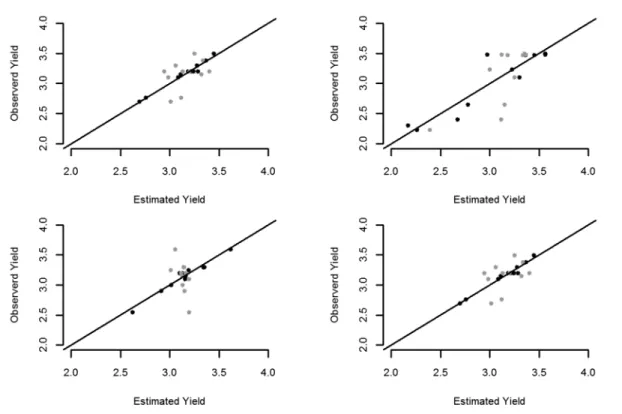
A comparison of estimated yield with official data is given in Figure 6, where the coefficient of determi-nation (R2) ranged from 0.96 to 0.98 for the correlation
masks approach; however, for the crop specific mask ap-proach, it only ranged between 0.02 and 0.67 (Table 4). The poor linear relationship between the estimated and official yield data is likely due to the EVI being influ-enced by other targets resulting in spectral mixture is-sues, especially when using low spatial resolution imag-es. This point was highlighted by Genovese et al. (2001), who showed improved estimates of yield values when the weighted NDVI eliminated noise. With the same
ob-jective, Maselli and Rembold (2001) and Kastens et al. (2005) applied the correlation maps in their study areas, since the aim was to use areas of a good relationship with yield data.
Kastens et al. (2005) reported that this technique is successfully employed in areas with sparse production. The eastern region in Paraná State has this characteristic, where municipalities have uneven relief, with the correlation masks approach estimating yield values close to the official data. This also helps to explain the significant errors generated by the model for this region using the crop specific mask.
Conclusions
This study also showed the limitations of crop specific masks to estimate yield especially with low spatial resolution images. The correlation maps proved to be more efficient at predicting yield since it is based on the relationship of EVI with crop yield, eliminating factors that could influence the results.
Acknowledgement
This research was funded by School of Agri-cultural Engineering, University of Campinas, by the Brazilian Federal Agency for Support and Evaluation of Graduate Education - CAPES (10745/12-2) and in part by the National Science Foundation EPSCoR (NSF EPS-0553722 and EPS-0919443) and KAN0061396/ KAN0066263. We also would like to thank the expert Felipe Ferreira Bocca for his help/advice in the statisti-cal analysis and R program, as well as Daniela Silva-Fuzzo and Mateus Santos for providing the crop specific mask for this study.
References
Alvares, C.A.; Stape, J. L.; Sentelhas, P.C.; Gonçalves, J. L.M.; Sparovek, G. 2013. Köppen’s climate classification map for Brazil. Meteorologische Zeitschrift, 22: 711–728.
Araújo, G.K.D.; Rocha, J.V.; Lamparelli, R.A.C.; Rocha, A.M. 2011. Mapping of summer crops in the state of Paraná, Brazil, through the 10-day spot vegetation ndvi composites. Engenharia Agrícola 31: 760-770.
Becker-Reshef, I.; Vermote, E.; Lindeman, M.; Justice, C. 2010. A generalized regression-based model for forecasting winter wheat yields in Kansas and Ukraine using MODIS data. Remote Sensing of Environment 114: 1312-1323.
Bolton, D.K.; Friedl, M.A. 2013. Forecasting crop yield using remotely sensed vegetation indices and crop phenology metrics. Agriculture and Forest Meteorology 173: 74-84.
Breusch, T.S.; Pagan, A.R. 1979. A simple test for heteroscedasticity and randon coefficient variation. Econometrica 47: 1287-1294. Companhia Nacional de Abastecimento [CONAB]. 2013. Brasilian
crop assessment: grains. Available at: http://www.conab.gov. br/OlalaCMS/uploads/arquivos/13_08_13_09_24_21_boletim_ ingles_julho_2013.pdf [Accessed Apr. 10, 2014]
Empresa Brasileira de Pesquisa Agropecuária [EMBRAPA]. 2011. MODIS products dataset. Available at: http://www.modis.cnptia. embrapa.br/geonetwork/srv/en/main.home [Accessed Aug. 10, 2010]. Esquerdo, J.C.D.M.; Zullo Júnior, J.; Antunes, J.F.G. 2011. Use of
NDVI/AVHRR time-series profiles for soybean crop monitoring in Brazil. International Journal of Remote Sensing 32: 3711-3727. Fernandes, J.L.; Rocha, J.V.; Lamparelli, R.A.C. 2011. Sugarcane
yield estimates using time series analysis of spot vegetation images. Scientia Agricola 68: 139-146.
Funk, C.; Budde, M.E. 2009. Phenologically-tuned MODIS NDVI-based production anomaly estimates for Zimbabwe. Remote Sensing of Environment 113: 115-125.
Genovese, G.; Vignolles, C.; Negre, T.; Passera, G. 2001. A methodology for a combined use of normalised difference vegetation index and CORINE land cover data for crop yield monitoring and forecasting: a case study on Spain. Agronomie 21: 91-111.
González-Sanpedro, M.C.; Le Toan, T.; Moreno, J.; Kergoat, L.; Rubio, E. 2008. Seasonal variations of leaf area index of agricultural fields retrieved from Landsat data. Remote Sensing of Environment 112: 810-824.
Gusso, A.; Ducati, J.R.; Veronez, M.R.; Arvor, D. 2013. Spectral model for soybean yield estimate using. International Journal of Geosciences 4: 1233-1241.
Huang, J.; Wang, H.; Dai, Q.; Han, D. 2014. Analysis of NDVI data for crop identification and yield estimation. IEEE Journal of Selected Topics in Applied Earth Observations and Remote Sensing 7: 4374-4384.
Huete, A.; Didan, K.; Miura, T.; Rodriguez, E.; Gao, X.; Ferreira, L. 2002. Overview of the radiometric and biophysical performance of the MODIS vegetation indices. Remote Sensing of Environment 83: 195-213.
Instituto Agronômico do Paraná [IAPAR]. 2013. Agricultural zoning = Zoneamento agrícola. Available at: http://www.iapar. br/modules/conteudo/conteudo.php?conteudo=1043 [Accessed Dec. 5, 2013] (in Portuguese).
Kastens, J.; Kastens, T.; Kastens, D.; Price, K.; Martinko, E.; Lee, R. 2005. Image masking for crop yield forecasting using AVHRR NDVI time series imagery. Remote Sensing of Environment 99: 341-356.
Maselli, F.; Rembold, F. 2001. Analysis of GAC NDVI data for cropland identification and yield forecasting in mediterranean African countries. Photogrammetric Engineering & Remote Sensing 67: 593-602.
Mkhabela, M.S.; Bullock, P.; Raj, S.; Wang, S.; Yang, Y. 2011. Crop yield forecasting on the Canadian prairies using MODIS NDVI data. Agriculture and Forest Meteorology 151: 385-393. National Aeronautics and Space Administration [NASA]. 2013a.
MODIS land mission. Available at: http://modis-land.gsfc.nasa. gov/index.html [Accessed Dec 2, 2013].
National Aeronautics and Space Administration [NASA]. 2013b. MODIS specification. Available at: http://modis.gsfc.nasa.gov/ about/specifications.php [Accessed Dec 2, 2013].
Picoli, M.C.A.; Lamparelli, R.A.C.; Sano, E.E.; Rocha, J.V. 2014. The use of alos/palsar data for estimating sugarcane productivity. Engenharia Agrícola 34: 1245-1255.
Rasmussen, M.S. 1992. Assessment of millet yields and production in northern Burkina Faso using integrated NDVI from the AVHRR. International Journal of Remote Sensing 13: 3431-3442.
Ren, J.; Chen, Z.; Zhou, Q.; Tang, H. 2008. Regional yield estimation for winter wheat with MODIS-NDVI data in Shandong , China. International Journal of Applied Earth Observation and Geoinformation 10: 403-413.
Shao, Y.; Campbell, J.B.; Taff, G.N.; Zheng, B. 2015. An analysis of cropland mask choice and ancillary data for annual corn yield forecasting using MODIS data. International Journal of Applied Earth Observation and Geoinformation 38: 78-87. Shapiro, S.S.; Wilk, M.B. 1965. An analysis of variance test for
normality (complete samples). Biometrika 52: 591-611. Tucker, C.J.; Holben, B.N.; Elgin, J.H.; McMurtrey, J.E. 1980.
Relationship of spectral data to grain yield variation. Photogrammetric Engineering & Remote Sensing 45: 657-666. United States Department of Agriculture [USDA]. 2005. Global
soil regions map. Available at: at: http://www.nrcs.usda. gov/wps/portal/nrcs/detail/vt/soils/?cid=nrcs142p2_054013 [Accessed Jan 6, 2015].
Wall, L.; Larocque, D.; Léger, P.M. 2008. The early explanatory power of NDVI in crop yield modelling. International Journal of Remote Sensing 29: 2211-2225.