ISSN 1546-9239
© 2012 Science Publication
Corresponding Author: Thamilselvan, R., Department of Computer Science and Engineering, Kongu Engineering College, Perundurai, Erode 638 052, Tamilnadu, India
Hybridization of Genetic Algorithm with Parallel
Implementation of Simulated Annealing for Job Shop Scheduling
Thamilselvan Rakkiannan and Balasubramanie Palanisamy
Faculty of Computer Science and Engineering,
Kongu Engineering College, Perundurai, Erode 638 052, Tamilnadu, India
Abstract: Problem statement: The Job Shop Scheduling Problem (JSSP) is observed as one of the most difficult NP-hard, combinatorial problem. The problem consists of determining the most efficient schedule for jobs that are processed on several machines. Approach: In this study Genetic Algorithm (GA) is integrated with the parallel version of Simulated Annealing Algorithm (SA) is applied to the job shop scheduling problem. The proposed algorithm is implemented in a distributed environment using Remote Method Invocation concept. The new genetic operator and a parallel simulated annealing algorithm are developed for solving job shop scheduling. Results: The implementation is done successfully to examine the convergence and effectiveness of the proposed hybrid algorithm. The JSS problems tested with very well-known benchmark problems, which are considered to measure the quality of proposed system. Conclusion/Recommendations: The empirical results show that the proposed genetic algorithm with simulated annealing is quite successful to achieve better solution than the individual genetic or simulated annealing algorithm.
Key words: Job shop scheduling, genetic algorithm, simulated annealing
INTRODUCTION
Meta-heuristics is used to solve with the computationally hard optimization problems. Meta-heuristics consist of a high level algorithm that guides the search using other particular methods. Meta-heuristics can be used as a standalone approach for solving hard combinatorial optimization problems. But now the standalone approach is drastically changed and attention of researchers has shifted to consider another type of high level algorithms, namely hybrid algorithms. There are at least two issues has to be considered while combining more than one meta-heuristics: (a) how to choose the meta-heuristic methods and (b) how to combine the chosen heuristic methods into new hybrid approaches. Unfortunately, there are no theoretical foundations for these issues. For the former, different classes of search algorithms can be considered for the purposes of hybridization, such as exact methods, simple heuristic methods and meta-heuristics. Moreover, meta-heuristics themselves are classified into local search based methods, population based methods and other classes of nature inspired meta-heuristics. Therefore, in principle, one could combine any methods from the same class or methods from different classes. Our hybrid approach combines
Genetic Algorithms (GAs) and Simulated Annealing (SA) methods. Roughly, our hybrid algorithm runs the GA as the main algorithm and calls SA procedure to improve individuals of the population.
The rest of the paper is organized as follows. The description of JSSP problem is followed by the introduction. Followed by there is a discussion about the literature review. In the fourth part, GA and SA methodologies are given for job shop scheduling. Finally the implementation of the HGAPSA to the JSSP is given with the algorithm using the proposed method with the experimental results and a discussion of the proposed method and a conclusion and future enhancement is also given.
Job Shop scheduling problem: The n×m Job Shop Scheduling problem labeled by the symbol n, m, J, O, G and Cmax. It can be described by the finite set of n jobs J
= {j0, j1, j2, j3,…..jn, jn+1} (the operation 0 and n+1 has
duration and represents the initial an final operations), each job consist of a chain of operations O = {o1,o2,o3,….om}, Each operation has processing time
{ʎi1, ʎi2, ʎi3,…. ʎim}, finite set of m machines M = {m1,
m2, m3….mm}, G is the matrix that represents the
processing order of job in different machines and Cmax
the last operation in job shop. On O define A, a binary relation representing precedence between operations. If (v, u)∈A then u has to be performed before v. A schedule is a function S: 0→IN∪{0} that for each operation u defines a start time S(u). A schedule S is feasible if Eq. 1-3:
u 0 : S(u) 0
∀ ∈ ≥ (1)
u, v 0,(u, v) A : S(u) (u) S(v)
∀ ∈ ∈ + λ ≤ (2)
u, v O, u v, M(v) M(v) : S(u)
(u) S(v) or S(v) (v) S(u)
∀ ∈ ≠ = +
λ ≤ + λ ≤ (3)
The length of a schedule S is Eq. 4:
len (S) = maxv∈o(S(u)+λ(u)) (4)
The goal is to find an optimal schedule, a feasible schedule of minimum length, min (len(S)).
An instance of the JSS problem can be represented by means of a disjunctive graph G = (O, A, E). Here O is the vertex which represents the operations and A represents the conjunctive arc which represents the priority between the operations and the edge in E = {(u, v)|u, v∈O, u≠v, M (u) = M(v)} represent the machine capacity constraints. Each vertex u has a weight, equal to the processing time ʎ(u). Let us consider the bench mark problem of the JSSP with four jobs, each has three different operations and there are three different machines. Operation sequence, machine assignment and processing time are given in Table 1.
Based on the above bench mark problem, we create a matrix G, in which rows represent the processing order of operation and the column represents the processing order of jobs. Also we create a matrix P, in which row i represents the processing time of Ji for different operations:
1 2 3
3 2 1
2 3 1
1 3 2
2 3 4
M M M
4 4 1
M M M
G P
2 2 1
M M M
3 3 1
M M M
= =
The processing time of operation i on machine j is represented by Oij. Let ʎij be the processing time of Oij in
the relation Oij→ Oij. Cij represents the completion of
the operation Oij. So that the value Cij = Cik + ʎij
represents the completion time of Oij. The main
objective is to minimize of Cmax. It can be calculated as
Eq. 5:
max all ij ij
C =max O ∈O(C ) (5)
The distinctive graph of the above bench mark job scheduling problem is shown in Fig. 1, in which vertices represents the operation. Precedence among the operation of the same job is represented by Conjunctive arc, which are doted directed lines. Precedence among the operation of different job is represented by Disjunctive arc, which areundirected solid lines. Two additional vertices S and E represents the start and end of the schedule.
The Gantt Chart of the above bench mark job scheduling problem is shown in Fig. 2. Gantt Chart is the simple graphical representation technique for job scheduling. It simply represents a graphical chart for display schedule; evaluate makespan, idle time, waiting time and machine utilization.
Literature review: Many researchers are working in job shop scheduling problem. Garey et al. (1976) were the first who introduced job shop scheduling problems. Some researchers like Brandimart (1993) and Paulli (1995) have used dispatching rules for solving flexible job shop scheduling problems. Attention to size proved that job shop scheduling problems are NP-Hard (Garey et al., 1976) and with added flexibility increase complexity more than job shop. Ram et al. (1996) have applied a parallel simulated annealing for job shop scheduling, but the same temperature is maintained in all the machines. Bozejko et al. (2009) have proposed the parallel simulated annealing for the job shop scheduling. But the same sequential algorithm is implemented more than one machine in a parallel order. Ramkumar et al. (2012) proposed real time fuzzy logic for job shop scheduling problem.
Table 1: Processing time and sequence for 4×3 problem instance Operation number and Machine Processing Job processing sequence assigned time
Start operation 0 -- 0
(Dummy)
J1 O11 M1 2
O12 M2 3
O13 M3 4
J2 O21 M3 4
O22 M2 4
O23 M1 1
J3 O31 M2 2
O32 M3 2
O33 M1 3
J4 O41 M1 3
O42 M3 3
O43 M2 1
End operation 0 -- 0
Fig. 1: Illustration of disjunctive graph
Fig. 2: A Schedule of Gantt Chart for 4×3 problem Instance
Objective of JSP problem is to find the optimal schedule with minimum makespan, but this result is not clearly shown by author. Thamilselvan and Balasubramanie (2011; 2012) have used the various crossover strategies for genetic algorithm for JSSP and integration of Genetic algorithm with Tabu Search for the JSSP. The above two methods were efficient for the small size JSP problems. Mohamed (2011) proposed a genetic algorithm for JSSP, but this algorithm is efficient only for less number of jobs. The ratio scheduling algorithm to solve the allocation of jobs in the shop floor was proposed by Hemamalini et al. (2010). This algorithm is more efficient when the result for the bench mark instances when the due date is less than half of the total processing time.
MATERIALS AND METHODS
Genetic algorithm: Genetic algorithms are probabilistic meta-heuristic technique, which may be used to solve computationally hard optimization problems. They are based on the genetic process of chromosome. Over many generations, natural
populations evolve according to the principles of natural selection of genes, i.e., survival of the fittest, first clearly stated by Charles Darwin in The Origin of Species. There is a initial solution as a Population to start the process and it filled with different order of chromosome. The chromosome consists of collection genes. Job is represented by each gene in chromosome and the job sequence in a schedule based on the position of the gene. GA uses Crossover and Mutation operation to generate a new population. By crossover operation, GA generates the neighborhood to explore new feasible solution.
Fig. 3: A standard genetic algorithm
The structure of a genetic algorithm for the scheduling problem can be divided into four parts: the choice of representation of individual in the population; the determination of the fitness function; the design of genetic operators; the determination of probabilities controlling the genetic operators. Yamada and Nakano (1997) was implemented the GA for the job shop scheduling problems.
Sequential Simulated Annealing (SSA): SSA belongs to the type of local search algorithms (Eglese, 1990). SA algorithm is inspired metal cooling process. In this process, the temperature is gradually reduced to reach the optimal solutions. SA algorithm searches current solution neighborhoods for a better solution and uses it for many complementary problems. Some researchers like Fattahi et al. (2007; 2009) and Zandieh et al. (2008) used SA algorithm in flexible job shop environment. SA algorithm generates an initial solution randomly. A neighbor of this solution is then generated by a suitable mechanism and the change in the cost function is calculated. If a decrease in the cost function is obtained, the current solution is replaced by the generated neighbor. If the cost function fun of the neighbor is greater, the newly generated neighbor replaces the current solution with an acceptance probability function given in Eq. 6:
d P(d,T) exp( )
T
= − (6)
Where:
d=Cs[ j] Cs[i]−
CS[i] and CS[j] are the cost function generated state
and the present state respectively. T is the temperature
to control the annealing process. The above equation implies that a small increase in fun are more likely to be accepted than large increases in the fun and also that when T is high, most of the newly generated neighbors are accepted. However, most of the cost increasing transactions are rejected if T approaches zero. Initially the temperature of the SA algorithm is kept as high so that the algorithm proceeds by generating a certain number of neighbors at each temperature, while the temperature parameter is gradually dropped. This algorithm leads to an optimal solution. The typical procedure for SSA algorithm is shown in Fig. 4.
For SSA the initial schedule is generated from a disjunctive graph G for solving job shop scheduling problem. The Giffer and Thompson (1960) algorithm is used to find the initial schedule. This algorithm obtains the schedule with all the operations (n) and all the machines (m) with the criteria employed being the earliest starting time and the processing time of each of the operations. The operation not yet included in the partial schedule at each stage, if the minimum time is chosen. If all the operations are included in the schedule, then the partial schedule becomes a complete schedule. The generated complete schedule can be represented in a diagraph.
The earliest and the latest start time of each operations in a diagraph are calculated after obtain the diagraph with all the operations. The critical path is used to find the earliest and latest start time. The earliest start time or the latest start time of the last operation is known as the makespan. This is the cost of the schedule (Krishna et al., 1995).
Fig. 4: A standard simulated annealing algorithm
Fig. 5: Permutation of operations on a critical block
• The earliest start time and latest start of each vertex on the edge must be the same
• For the same edge u→v, the operation time and the sum of the start time of u must be equal to the start time of v
Neighborhood of a schedule S can be defined as a set of schedules that can be obtained by applying the transition operator on the given schedule S (Li-Ning et al., 2009). The transition operator permutes the order of operations in a critical block by moving an operation to the beginning or end of the critical block, thus forming the CB neighborhood. In this neighborhood, the distance between S and any element in N(S) can vary depending on the position of the moving operation. It has been experimentally shown in (Yamada et al.,
1994) that SA using the CB neighborhood is more powerful than SA using the AS neighborhood. Thus, the CB neighborhood may as well be investigated in the GA context. Figure 5 illustrates how the two transition operators work.
The main objective function of the proposed algorithm is to minimize the makespan. We use the second approach for solving job shop scheduling problem. The procedure SA_Parallel() generate an initial schedule S[i] and then the algorithm is parallelly running on different machines. Let N be the total number of iterations in each SA algorithm temperature, S[j] is the neighbourhood of S[i], Bc is best known
solution cost, Bs is the best known schedule of JSSP. As
mentioned earlier, the given scheduling algorithm to schedule operations on machines. The generated S[j] is the input to the scheduling algorithm and then the algorithm compute the cost of S[j] as CS[j]. The cost of
the new schedule is compared with the cost of the initial schedule to process the algorithm.
Procedure: SA_Parallel() Input:
temperature T, starting temperature Ts, ending temperature Te, number of iteration N.
Begin
generate initial schedule S[i].
compute the cost CS[i] of initial schedule S[i].
n=1, T=Ts. while T<Te while n<N
select neighbourhood S[j] of S[i].
compute the cost CS[j] of the new schedule S[j].
compute = Cs[j]-Cs[i] .
if δ≤0 then S[i]=S[j]. CS[i]=CS[j].
else
generate a random variable R∼(0, 1). if exp (-δ/T)>R
S[i]=S[j]. CS[i]=CS[j].
end if end if n=n+1. end while T= T*0.995. end while if CS[i]<Bc
Bc=CS[i].
Bs=S[i].
end if End
The implementation of the above algorithm is done by a server machine and a set of client machines. The server node generates the initial schedule S[i], the processing times of all the operations and the machine
order for each job. This server machine then sends the initial schedule and different range of temperature parameters to each of the client machines on the network. Each client machine has its maximum temperature Ts and minimum temperature Te. The client
machines execute the above algorithm with different range of temperature and send the solution to the server machine. After receiving the solutions from the client machines, the server machine selects the best solution with the minimal makespan.
Hybrid Genetic Algorithm with Parallel Simulated Annealing (HGAPSA): Parallel implementation of SA generates a better solution with faster convergence. Initially, n number of client machines processes the SA algorithm with different initial schedule. After the fixed number of iterations, the client machines are exchange the results with the server machine to get the best schedule.
In genetic algorithm, an initial population consisting of a set of schedule is selected and then the schedules are evaluated. Relatively more effective schedule are selected to have more off springs, where are in some way, related to the original solutions. The performance of the genetic algorithm depends on the crossover operation. If it is properly selected, the final population will produce the better solution. Simulated annealing algorithm aims to produce such a solution. For the parallel SA implementation, we need good initial solutions for the fast convergence of SA. GA will produce a good number of initial solutions. The operator used for generating off springs in job shop scheduling is related to the processing order of jobs on different machines of the two parent solutions.
We introduce new cross over strategy named as Unordered Subsequence Exchange Crossover (USXX) that children inherit subsequences on each machine as far as possible from parents. Unordered Subsequence exchange crossover creates a new children’s even the subsequence of parent1 is not in the same order in parent 2. The algorithm for USXX is as follows:
Step 1: Generate two random parent individual namely P1 and P2 with a sequence of all operations.
Step 2: Generate two child individual namely C1 and C2.
Step 3: Select random subset of operations (genes) from P1 and copy it into C1.
Step 5: The remaining operations of P2 that are not in the subset can be filled in C1 so as to maintain their relative ordering.
Procedure: HGAPSA_Server() Input: Initialize number of iterations Ni. Begin
iter = 1. while iter< = Ni
server machine generates a n initial solutions S[1], S[2],…S[n] using GA.
for i = 1 to n
assign S[i] to Ci where Ci is the ith client machine.
each Ci run SA_Parallel() algorithm using S[i].
after getting the best solution, client machine send it to server machine.
end for iter=iter+1. end while End
The above GA and PSA algorithms are implemented in a network of one server and five workstations. The server node use GA to generates n number of initial schedule and assigns those schedules to the n number of client machines as an initial solution. The genetic algorithm starts with an initial schedule and then it performs USXX crossover operation to update the population. This process has to be repeated number of times. The client machine use SA_Parallel()procedure to find the best schedule and then the best schedule is send to the server machine.
RESULTS AND DISCUSSION
The performance of the proposed HGAPSA algorithm is compared with the Genetic Algorithm (GA), Sequential Simulated Annealing (SSA) Algorithm and Parallel Simulated Annealing (PSA) for standard JSP test instances of Lawrence (1984) instances from LA30 to LA40 and Storer et al. (1992) instances SWV11-SWV20.
Table 2 shows comparison of makespan value produced from different algorithms for problem instances LA30-LA40 (Lawrence, 1984) Column 1 specifies the problem instances, Column 2 specifies the number of jobs, Column 3 shows the number of machines, Column 4 specify the optimal value for each problem. Column 5, 6, 7 and 8 specify results from SA, SSA, PSA and HGAPSA respectively. It shows that the proposed hybrid algorithm has succeeded in getting the optimal solutions for all the problems.
Figure 6 shows average makespan value generated by GA, SSA, PSA and HGAPSA for different problem instances of Lawrence (1984). It also shows that SSA produce the worst result compare to other two algorithms and the HGAPSA algorithm is better than the other two algorithms. Figure 7 shows the comparison of Average Relative Error for all the three methods. It clearly shows that the Average Relative Error for HGAPSA is 0.13 Table 3 shows comparison of makespan value produced from different algorithms for problem instances SWV11-SWV20 (Storer et al., 1992) Column 1 specifies the problem instances, Column 2 specifies the number of jobs, Column 3 shows the number of machines, Column 4 specify the optimal value for each problem. Column 5, 6, 7 and 8 specify results from SA, SSA, PSA and HGAPSA respectively. It shows that the proposed hybrid algorithm has succeeded in getting the optimal solutions for all the problems.
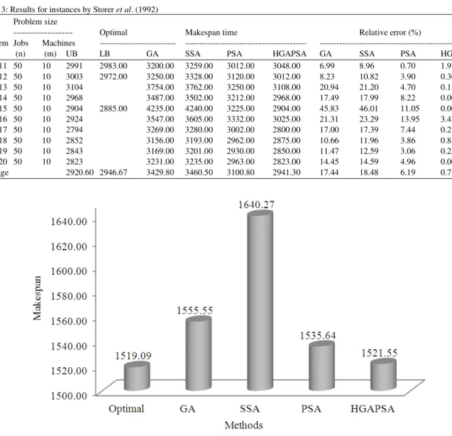
Figure 8 shows average makespan value generated by GA, SSA, PSA and HGAPSA for different problem instances of Storer et al. (1992). It also shows that SSA produce the worst result compare to other two algorithms and the HGAPSA algorithm is better than the other two algorithms. Figure 9 shows the comparison of Average Relative Error for all the three methods. It clearly shows that the Average Relative Error for HGAPSA is 0.17.
Typical runs of problem instances LA30 (Lawrence, 1984) are illustrated in Fig. 10 by the GA, SSA, PSA and HGAPSA. The graph shows that the proposed HGAPSA reach the optimal solution faster than other two methods. For LA30, GA, SSA and PSA never produces the best known solution. But HGAPSA produced the optimal solution with 2000 iterations. We have tested with 5000 iterations, but other algorithms does not produce a optimal solution.
Typical runs of problem instances SWV15 (Storer et al., 1992) are illustrated in Fig. 11 by the GA, SSA, PSA and HGAPSA. The graph shows that the proposed HGAPSA reach the optimal solution faster than other two methods. For SWV15, GA, SSA and PSA never produces the best known solution. But HGAPSA produced the optimal solution with 2500 iterations. We have tested with 6000 iterations, but other algorithms does not produce a optimal solution.
Table 2: Results for instances by Lawrence (1984) Problem size
--- Makespan ttime Relative error (%)
Problem Jobs Machines --- --- Name (n) (m) Optimal GA SSA PSA HGAPSA GA SSA PSA HGAPSA LA30 20 10 1355.00 1398.00 1430.00 1360.00 1355.00 3.17 5.54 0.37 0.00 LA31 30 10 1784.00 1829.00 1950.00 1800.00 1790.00 2.52 9.30 0.90 0.34 LA32 30 10 1850.00 1877.00 2126.00 1875.00 1860.00 1.46 14.92 1.35 0.54 LA33 30 10 1719.00 1820.00 2006.00 1740.00 1719.00 5.88 16.70 1.22 0.00 LA34 30 10 1721.00 1810.00 1945.00 1742.00 1725.00 5.17 13.02 1.22 0.23 LA35 30 10 1888.00 1950.00 2105.00 1953.00 1895.00 3.28 11.49 3.44 0.37 LA36 15 15 1279.00 1279.00 1305.00 1285.00 1279.00 0.00 2.03 0.47 0.00 LA37 15 15 1408.00 1441.00 1453.00 1423.00 1408.00 2.34 3.20 1.07 0.00 LA38 15 15 1219.00 1220.00 1220.00 1219.00 1219.00 0.08 0.08 0.00 0.00 LA39 15 15 1246.00 1246.00 1255.00 1250.00 1246.00 0.00 0.72 0.32 0.00 LA40 15 15 1241.00 1241.00 1248.00 1245.00 1241.00 0.00 0.56 0.32 0.00 Average 1519.09 1555.55 1640.27 1535.64 1521.55 2.17 7.05 0.97 0.13
Table 3: Results for instances by Storer et al. (1992) Problem size
--- Optimal Makespan time Relative error (%)
Problem Jobs Machines --- --- --- Name (n) (m) UB LB GA SSA PSA HGAPSA GA SSA PSA HGAPSA SWV11 50 10 2991 2983.00 3200.00 3259.00 3012.00 3048.00 6.99 8.96 0.70 1.91 SWV12 50 10 3003 2972.00 3250.00 3328.00 3120.00 3012.00 8.23 10.82 3.90 0.30 SWV13 50 10 3104 3754.00 3762.00 3250.00 3108.00 20.94 21.20 4.70 0.13 SWV14 50 10 2968 3487.00 3502.00 3212.00 2968.00 17.49 17.99 8.22 0.00 SWV15 50 10 2904 2885.00 4235.00 4240.00 3225.00 2904.00 45.83 46.01 11.05 0.00 SWV16 50 10 2924 3547.00 3605.00 3332.00 3025.00 21.31 23.29 13.95 3.45 SWV17 50 10 2794 3269.00 3280.00 3002.00 2800.00 17.00 17.39 7.44 0.21 SWV18 50 10 2852 3156.00 3193.00 2962.00 2875.00 10.66 11.96 3.86 0.81 SWV19 50 10 2843 3169.00 3201.00 2930.00 2850.00 11.47 12.59 3.06 0.25 SWV20 50 10 2823 3231.00 3235.00 2963.00 2823.00 14.45 14.59 4.96 0.00 Average 2920.60 2946.67 3429.80 3460.50 3100.80 2941.30 17.44 18.48 6.19 0.71
Fig. 7: Average relative error values by different algorithms for LA30-LA40
Fig. 8: Average makespan values by different algorithms for SWV11-SWV20
Fig. 10: The time evolutions of makespans for the LA30 (20 jobs and 10 machines)
Fig. 11: The time evolutions of makespans for the SWV15 (50 jobs and 10 machines)
Table 4: Computational time for LA30-LA40 and SWV11-SWV20 Problem size
--- Makespan (CPU time)
Problem Jobs Machines ---
Name (n) (m) Optimal GA SSA PSA HGAPSA
LA30 20 10 1355 1398(2539) 1430(3152) 1360(1925) 1355(1554) LA31 30 10 1784 1829(2780) 1950(3750) 1800(2532) 1790(2106) LA32 30 10 1850 1877(2850) 2126(4104) 1875(2585) 1860(2151) LA33 30 10 1719 1820(2829) 2006(4007) 1740(2581) 1719(1922) LA34 30 10 1721 1810(2971) 1945(3945) 1742(2625) 1725(2051) LA35 30 10 1888 1950(2920) 2105(4398) 1953(2453) 1895(2264) LA36 15 15 1279 1279(1978) 1305(2585) 1285(1615) 1279(1432) LA37 15 15 1408 1441(2752) 1453(3485) 1423(2125) 1408(1659) LA38 15 15 1219 1220(1885) 1220(2423) 1219(1598) 1219(1264) LA39 15 15 1246 1246(1800) 1255(2540) 1250(1605) 1246(1351) LA40 15 15 1241 1241(1752) 1248(2408) 1245(1620) 1241(1337) SWV11 50 10 2991 3200(4438) 3259(5632) 3012(3625) 3048(3184) SWV12 50 10 3003 3250(5235) 3328(6780) 3120(3882) 3012(3537) SWV13 50 10 3104 3754(5498) 3762(7720) 3250(4250) 3108(3691) SWV14 50 10 2968 3487(4531) 3502(5751) 3212(3632) 2968(3177) SWV15 50 10 2904 4235(4427) 4240(5675) 3225(3421) 2904(3124) SWV16 50 10 2924 3547(4513) 3605(5712) 3332(3438) 3025(3149) SWV17 50 10 2794 3269(3900) 3280(4520) 3002(3185) 2800(2870) SWV18 50 10 2852 3156(4104) 3193(4732) 2962(3278) 2875(3037) SWV19 50 10 2843 3169(4098) 3201(4532) 2930(3185) 2850(2964) SWV20 50 10 2823 3231(4075) 3235(4572) 2963(3004) 2823(2832)
Table 5: Average makespan and Computational time for LA30-LA40 and SWV11-SWV20 Average makespan (Average CPU time)
No of ---
Problem Name problems GA SSA PSA HGAPSA
LA30- LA40 11 1555.55 (2459.64) 1640.27 (3345.18) 1535.64 (2114.91) 1521.55 (1735.55) SWV11- SWV20 10 3429.80 (4481.90) 3460.50 (5562.60) 3100.80 (3490.00) 2941.30 (3156.50)
CONCLUSION
In this study integration of genetic algorithm with parallel simulated annealing algorithm is implemented for job shop scheduling. The implementation has been done in a client server environment with the well-known benchmark problems. The results of the proposed algorithm are compared with the other standard meta-heuristic algorithms. It shows that the proposed algorithm is quite successful for the large size problems compare to other algorithms. Even the proposed algorithm produce the better result, there is a ambiguity in the population size. This problem needs to be addressed in the future. Also more than two meta-heuristic algorithms may be interpreted to improve the solution space.
REFERENCES
Bozejko, W., J. Pempera and C. Smuntnicki, 2009. Parallel simulated annealing for the job shop scheduling problem. Comput. Sci., 5544: 631-640. DOI: 10.1007/978-3-642-01970-8_62
Brandimart, P., 1993. Routing and scheduling in a flexible job shop by tabu search. Annal. Operat. Res., 41: 157-183. DOI: 10.1007/BF02023073
Eglese, R.W., 1990. Simulated annealing: A tool for operational research. Euo. J. Operation Res., 46: 271-281.
Fattahi, P, F. Jolai and J. Arkat, 2009. Flexible job shop scheduling with overlapping in operations. Appl. Math. Model., 33: 3076-3087. DOI: 10.1016/j.apm.2008.10.029, 2008
Fattahi, P., M.S. Mehrabad and F. Jolai, 2007. Mathematical modeling and heuristic approaches to flexible job shop scheduling problems. J. Intell. Manuf., 18: 331-342. DOI: 10.1007/s10845-007-0026-8 Garey, M.R., D.S. Johnson and R. Sethi, 1976. The
complexity of flowshop and jobshop scheduling. Math. Operat. Res., 1: 117-129. DOI: 10.1287/moor.1.2.117
Giffer, B. and G.L. Thompson, 1960. Algorithms for solving production-scheduling problems. Operat. Res., 8: 487-503. DOI: 10.1287/opre.8.4.487 Hemamalini, T., A. N.Senthilvel and S. Somasundaram,
2010. Scheduling algorithm to optimize jobs in shop floor. J. Math. Stat., 6: 416-420. DOI: 10.3844/jmssp.2010.416.420
Lawrence, S., 1984. Supplement to resource constrained project scheduling: An experimental investigation of heuristic scheduling techniques. Li-Ning, X., Y.W. Chen and K.W. Yang, 2009. An
efficient search method for multi-objective flexible job shop scheduling problems. J. Intell. Manuf., 20: 283-293. DOI: 10.1007/s10845-008-0216-z Mohamed, A.A.F., 2011. A genetic algorithm for
scheduling n jobs on a single machine with a stochastic controllable processing, tooling cost and earliness-tardiness penalties. Am. J. Eng. Applied
Sci., 4: 341-349. DOI:
10.3844/ajeassp.2011.341.349
Paulli, J., 1995. A hierarchical approach for the FMS scheduling problem. Eur. J. Operat. Res., 89: 32-425. DOI: 10.1016/0377-2217(95)00059-Y Ram, D.J., T.H. Sreenivas and K.G. Subramaniam,
1996. Parallel simulated annealing algorithms. J. Parallel Distributed Comput., 37: 207-212. Ramkumar, R., A. Tamilarasi and T. Devi, 2012. A
real time practical approach for multi objective job shop scheduling using fuzzy logic approach. J. Comput. Sci., 8: 606-612. DOI: 10.3844/jcssp.2012.606.612
Storer, R.H., S.D. Wu and R. Vaccari, 1992. New search spaces for sequencing problems with application to job shop scheduling. Manage. Sci., 38: 1495-1509.
Thamilselvan, R. and P. Balasubramanie, 2011. Analysis of various alternate crossover strategies for genetic algorithm to solve job shop scheduling problems. Eur. J. Sci. Res., 64: 538-554.
Thamilselvan, R., P.Balasubramanie, 2012. Integration of genetic algorithm with tabu search for job shop scheduling with unordered subsequence exchange crossover. J. Comput. Sci., 8: 681-693. DOI: 10.3844/jcssp.2012.681.693
Yamada, T. and R. Nakano, 1997. Genetic algorithms for job-shopscheduling problems. Proceedings of Modern Heuristic for Decision Support, Mar. 18-19, UNICOM Seminar, London, pp: 67-81. Yamada, T., B.E. Rosen and R. Nakano, 1994. A
simulated annealing approach to job shop scheduling using critical block transition operators. Proceedings of the IEEE International Conference on Neural Networks, IEEE World Congress on Computational Intelligence, Jun. 27-Jul. 2, IEEE Xplore Press, Orlando, FL., pp: 4687-4692. DOI: 10.1109/ICNN.1994.375033