Genetic algorithms for the traveling salesman problem

Genetic algorithms for the

traveling salesman problem

Jean-Yves Potvin

Centre de Recherche sur les Transports, Universitd de Montrgal, C.P. 6128, Succ. Centre-Ville, Montrdal, Qudbec, Canada H3C 3J7

This paper is a survey of genetic algorithms for the traveling salesman problem.

Genetic algorithms are randomized search techniques that simulate some of the processes

observed in natural evolution. In this paper, a simple genetic algorithm is introduced,

and various extensions are presented to solve the traveling salesman problem. Computational

results are also reported for both random and classical problems taken from the operations

research literature.

Keywords:

Traveling salesman problem, genetic algorithms, stochastic search.

1.

Introduction

The Traveling Salesman Problem (TSP) is a classical combinatorial optimization

problem, which is simple to state but very difficult to solve. The problem is to find

the shortest tour through a set of N vertices so that each vertex is visited exactly once.

This problem is known to be NP-hard, and cannot be solved exactly in polynomial

time.

Many exact and heuristic algorithms have been developed in the field of

operations research (OR) to solve this problem. We refer readers to Bodin et al. [5],

Lawler et al. [35], Laporte [34] for good overviews of the TSP. In the sections that

follow, we briefly introduce the OR problem-solving approaches to the TSP. Then,

the genetic algorithms are discussed.

1.1.

EXACT ALGORITHMS

The exact algorithms are designed to find the optimal solution to the TSP, that

is, the tour of minimal length. They are computationally expensive because they must

(implicitly) consider all solutions in order to identify the optimum. These exact

algorithms are typically derived from the integer linear programming (ILP) formulation

of the TSP

340

J.-Y. Potvin, The traveling salesman problem

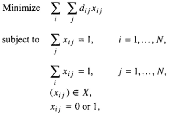
Minimize

~ , ~ , dijxij

subject to

~_~ xij = I,

i = 1 ... N,

Z

Xij

(Xij ) E X,

xij

j = l . . . N,

where N is the number of. vertices,

dij

is the distance between vertices i and j, and

the xij's

are the decision variables:

xij

is set to 1 when arc

(i,j)

is included in the tour,

and 0 otherwise.

(xij) E X

denotes the set of subtour-breaking constraints that restrict

the feasible solutions to those consisting of a single tour.

Although the subtour-breaking constraints can be formulated in many different

ways, one very intuitive formulation is

Z

Xij <<" S V I - 1 (S V C

V; 2

<-Isvl <-

_{N -}

_2),

i,j ~ Sv

where V is the set of all vertices,

S v

is some subset of V, and

[Sv[

is the cardinality

of

S v.

These constraints prohibit subtours, that is, tours on subsets with less than N

vertices. If there were such a subtour on some subset of vertices

Sv,

this subtour

would contain

I Svt

arcs. Consequently, the left-hand side of the inequality would be

equal to

I Svl,

which is greater than

I s v l -

1,

and the above constraint would be

violated for this particular subset. Without the subtour-breaking constraints, the TSP

reduces to an assignment problem (AP), and a solution like the one shown in figure 1

would then be feasible.

(b)

(

Figure 1.

(a)

the optimal value. This is true in particular for asymmetric problems, where dij ~ dji

for some

i,j.

For symmetric problems, like the Euclidean TSP (ETSP), the AP-

solutions often contain many subtours on two vertices. Consequently, these problems

are better addressed by specialized algorithms that can exploit their particular structure.

For instance, a specific ILP formulation can be derived for the symmetric problem

which allows for relaxations that provide sharp lower bounds (i.e., the well-known

one-tree relaxation [25]).

It is worth noting that problems with a few hundred vertices can now be

routinely solved to optimality. Moreover, instances involving more than 2000 vertices

have been recently addressed. For example, the optimal solution to a symmetric

problem with 2392 vertices was found after two hours and forty minutes of computation

time on a powerful vector computer, the IBM 3090/600 (Padberg and Rinaldi [50, 51 ]).

On the other hand, a classical problem with 532 vertices took five hours on the same

machine, indicating that the size of the problem is not the only determining factor

for computation time.

We refer the interested reader to [34] for a good account of the state-of-the-

art in exact algorithms.

1.2.

HEURISTIC ALGORITHMS

Running an exact algorithm for hours on a powerful computer may not be very

cost-effective if a solution, within a few percent of the optimum, can be found

quickly on a small microcomputer. Accordingly, heuristic or approximate algorithms

are often preferred to exact algorithms for solving the large TSPs that occur in

practice (e.g., drilling problems). Generally speaking, TSP heuristics can be classified

as tour construction procedures, tour improvement procedures, and composite procedures,

which are based on both construction and improvement techniques.

(a)

Construction procedures. The best known procedures in this class gradually

build a tour by selecting each vertex in turn and by inserting them one by one into

the current tour. Various measures are used for selecting the next vertex and for

identifying the best insertion place, like the proximity to the current tour and the

minimum detour (Rosenkrantz et al. [53]).

342

J.-Y. Potvin, The traveling salesman problem

i j i j

\ I I

\!

IIXx

1 k _{I k}

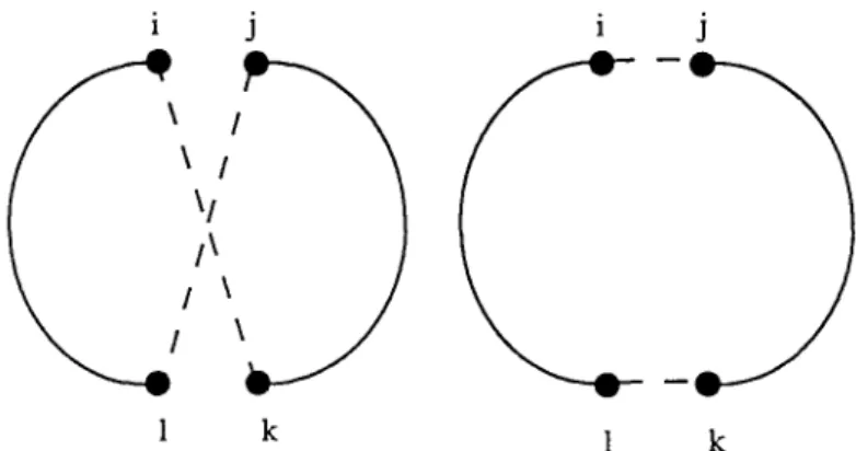
Figure 2. Exchange of links (i, k),(j, l) for links (i,j),(k, l).

Fiechter [11], Glover [16, 17], Johnson [30], Kirkpatrick et al. [32], Malek et al.

[40]). Basically, these new procedures allow local modifications that increase the

length of the tour. By these means, these methods can escape from local minima and

explore a larger number of solutions.

(c)

Composite procedures.

Recently developed composite procedures, which

are based on both construction and improvement techniques, are now among the most

powerful heuristics for solving TSPs. Among the new generation of composite heuristics,

the most successful ones are the CCAO heuristic (Golden and Stewart [19]), the

iterated Lin-Kernighan heuristic (Johnson [30]), and the GENIUS heuristic (Gendreau

et al. [15]).

For example, the iterated L i n - K e r n i g h a n heuristic can routinely find solutions

within 1% of the optimum for problems with up to 10,000 vertices [30]. Heuristic

solutions within 4% of the optimum for some 1,000,000-city ETSPs are also reported

in [3]. Here, the tour construction procedure is a simple greedy heuristic. At the start,

each city is considered as a fragment, and multiple fragments are built in parallel by

iteratively connecting the closest fragments together until a single tour is generated.

Then, the solution is processed by a 3-opt exchange heuristic. A clever implementation

of the above procedure solved some 1,000,000-city problems in less than four hours

on a VAX 8550. The key implementation idea is that most of the edges that are likely

to be added during the construction of the tour are not affected by the addition of

a new edge. Consequently, only a few calculations need to be performed from one

iteration to the next. Also, special data structures are designed to implement a priority

queue for the insertion of the next edge.

1.3.

GENETIC ALGORITHMS

have already been applied to the TSP. However, the "pure" genetic algorithm, developed

by Holland and his students at the University of Michigan in the '60s and '70s, was

not designed to solve combinatorial optimization problems. In those early days, the

application domains were mostly learning tasks and optimization of numerical functions.

Consequently, the original algorithm must be modified to handle combinatorial

optimization problems like the TSP.

This paper describes various extensions to the original algorithm to solve the

TSP. To this end, the remainder of the paper is organized along the following lines.

In sections 2 and 3, we first introduce a simple genetic algorithm and explain why

this algorithm cannot be applied to the TSP. Then, sections 4 to 9 survey various

extensions proposed in the literature to address the problem. Finally, section 10

discusses other applications in transportation-related domains.

A final remark concerns the class of TSPs addressed by genetic algorithms.

Although these algorithms have been applied to TSPs with randomly generated

distance matrices (Fox and McMahon [13]), virtually all work concerns the ETSP.

Accordingly, Euclidean distances should be assumed in the sections that follow,

unless it is explicitly stated otherwise.

2.

A simple genetic algorithm

This section describes a simple genetic algorithm. The vocabulary will probably

look a little bit "esoteric" to the OR specialist, but the aim of this section is to

describe the basic principles of the genetic search in the most straightforward and

simple way. Then, the next section will explain how to apply these principles to a

combinatorial optimization problem like the TSP.

At the origin, the evolution algorithms were randomized search techniques

aimed at simulating the natural evolution of asexual species (Fogel et al. [12]). In this

model, new individuals were created via random mutations to the existing individuals.

Holland and his students extended this model by allowing "sexual reproduction", that

is, the combination or crossover of genetic material from two parents to create a new

offspring. These algorithms were called "genetic algorithms" (Bagley [2]), and the

introduction of the crossover operator proved to be a fundamental ingredient in the

success of this search technique.

2.1.

UNDERLYING PRINCIPLES

344

J.-Y. Potvin, The traveling salesman problem

behavior o f the genetic search is first characterized. Then, section 2.2 will describe

a simple genetic algorithm in greater detail.

First, let us assume that some function f(x)

is to be maximized over the set

of integers ranging from 0 to 63. In this example, we ignore the obvious fact that

such a small problem could be easily solved through complete enumeration. In order

to apply a genetic algorithm to this problem, the variable x must first be coded as

a bit string. Here, a bit string of length 6 is chosen, so that integers between 0

(000000) and 63 (I 11111) can be obtained. The fitness of each chromosome is f ( x ) ,

where x is the integer value encoded in the chromosome. Assuming a population of

eight chromosomes, it is possible to create an initial population by randomly generating

eight different bit strings, and by evaluating their fitness, through f, as illustrated

in figure 3. For example, chromosome 1 encodes the integer 49 and its fitness is

f ( 4 9 ) = 90.

Chromosome 1:110001

Fitness:

90

Chromosome 2:010101

Fitness:

10

Chromosome 3:110101

Fitness:

100

Chromosome 4:100101

Fitness:

5

Chromosome 5:000011

Fitness:

95

Chromosome 6:010011

Fitness:

90

Chromosome 7:001100

Fitness:

5

Chromosome 8:101010

Fitness:

5

Figure 3. A population of chromosomes.

By looking at the similarities and differences between the chromosomes and

by comparing their fitness values, it is possible to hypothesize that chromosomes

with high fitness values have two 1 's in the first two positions, or two l's in the last

two positions. These similarities are exploited by the genetic search via the concept

of schemata (hyperplanes, similarity templates). A schema is composed of O's and

l's, like the original chromosomes, but with the additional "wild card" or "don't

care" symbol *, standing either for 0 or I. Via the don't care symbol, schemata

represent subsets of chromosomes in the population. For example, the schema 11 ****

contains chromosomes 1 and 3 in the population illustrated in figure 3, while schema

****11 contains chromosomes 5 and 6.

Two fundamental characteristics of schemata are the order and the defining

length, namely:

(1) The

order

is the number of positions with fixed values (the schema 11.*** is

of order 2, the schema 110,00 is of order 5).

A "building block" is a schema of low order, short defining length and above-

average fitness (where the fitness of a schema is defined as the average fitness of

its members in the population). Generally speaking, the genetic algorithm moves in

the search space by combining building blocks from two parent chromosomes to

create a new offspring. Consequently, the basic assumption at the core of the genetic

algorithm is that a better chromosome is found by combining the best features of two

good chromosomes. In the example above, genetic material (i.e. bits) would be

exchanged between a chromosome with two l's in the first two positions and a

chromosome with two 1 's in the last two positions in order to create an offspring with

two l's in the first two positions

two l's in the last two positions (in the hope

that the x value encoded in this chromosome would generate a h i g h e r f ( x ) value than

both of its parents). Hence, the two above-average building blocks 11.** and ***I1

are combined on a single chromosome to create an offspring with higher fitness.

2.2.

A SIMPLE GENETIC ALGORITHM

Based on the above principles, a simple "pure" genetic algorithm can b'e

defined. In the following description, many new terms are introduced. These terms

will be defined in sections 2.2.1 to 2.2.4.

Step

Step

Step

Step

Step

Step

Step

Step

Step

1. Create an initial population of P chromosomes (generation 0).

2. Evaluate the fitness of each chromosome.

3. Select P parents from the current population via proportional selection (i.e.,

the selection probability is proportional to the fitness).

4. Choose at random a pair of parents for mating. Exchange bit strings with

the one-point crossover to create two offspring.

5. Process each offspring by the mutation operator, and insert the resulting

offspring in the new population.

6. Repeat steps 4 and 5 until all parents are selected and mated (P offspring

are created).

7. Replace the old population of chromosomes by the new one.

8. Evaluate the fitness of each chromosome in the new population.

9. Go back to step 3 if the number of generations is less than some upper

bound. Otherwise, the final result is the best chromosome created during the

search.

346

J.-Y. Potvin, The traveling salesman problem

2.2.1. Selection probability (selection pressure)

The parent chromosomes are selected for mating via proportional selection,

also known as "roulette wheel selection". It is defined as follows.

1.

Sum up the fitness values of all chromosomes in the population.

2.

Generate a random number between 0 and the sum of the fitness values.

3.

Select the first chromosome whose fitness value added to the sum of the fitness

values of the previous chromosomes is greater than or equal to the random

number.

In the population of chromosomes illustrated in figure 3, the total fitness value

is 400. The first chromosome is chosen when the random number falls in the interval

[0, 90]. Similarly, chromosomes 2 to 8 are chosen if the random number falls in the

intervals (90, 100], (100, 200], (200, 205], (205,300], (300, 390], (390, 395] and

(395,400], respectively. Obviously, a chromosome with high fitness has a greater

probability of being selected as a parent (assimilating the sum of the fitness values

to a roulette wheel, a chromosome with high fitness covers a larger portion of the

roulette). Chromosomes with high fitness contain more above-average building blocks,

and are favored during the selection process. In this way, good solution features are

propagated to the next generation.

However, proportional selection has also some drawbacks. In particular, a

"super-chromosome" with a very high fitness value will be selected at almost each

trial and will quickly dominate the population. When this situation occurs, the population

does not evolve further, because all its members are similar (a phenomenon referred

to as "premature convergence"). To alleviate this problem, the rank of the fitness

values can be used as an alternative to the usual scheme (Whitley [66]). In this case,

the selection probability of a chromosome is related to its rank in the population,

rather than its fitness value. Accordingly, the selection probability of a super-chromo-

some becomes identical to the selection probability of any chromosome of rank 1 in

a given population.

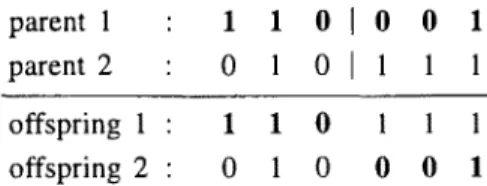
2.2.2. One-point crossover

The one-point crossover operator is aimed at exchanging bit strings between

two parent chromosomes. A random position between 1 and L - 1 is chosen along

the two parent chromosomes, where L is the c h r o m o s o m e ' s length. Then, the

chromosomes are cut at the selected position, and their end parts are exchanged to

create two offspring. In figure 4, for example, the parent chromosomes are cut at

position 3.

parent 1

:

parent 2

:

0

1 0 I 1 1 1

offspring 1 :

1 1 0

1 1 1

offspring 2 :

0

1 0

0 0 1

Figure 4. The one-point crossover.

generation to the next. The crossover rate can be related to the "aggressiveness" of

the search. High crossover rates create more new offspring, at the risk of losing many

good chromosomes in the current population. Conversely, low crossover rates tend

to preserve the good chromosomes from one generation to the next, via a more

conservative exploration of the search space. In [ 10], it is suggested that good performance

requires the choice of a fairly high crossover rate, such as 0.6, so that about 60%

of the selected parents will undergo crossover.

Various extensions to the one-point crossover are also reported in the literature.

For example, the two-point crossover selects two cut points at random on both

parent chromosomes, and exchanges the substring located between the two cut

points. Other generalizations, like the M-point crossover and the uniform crossover

(Syswerda [57]), may be found in the literature, but their description would be

beyond the scope of this paper.

2.2.3. Mutation

The bits of the two offspring generated by the one-point crossover are then

processed by the mutation operator. This operator is applied to each bit with a small

probability (e.g., 0.001). When it is applied at a given position, the new bit value

switches from 0 to 1 or from 1 to 0. The aim of the mutation operator is to introduce

random perturbations into the search process. It is useful, in particular, to introduce

diversity in homogeneous populations, and to restore bit values that cannot be recovered

via crossover (e.g., when the bit value at a given position is the same for every

chromosome in the population). Accordingly, it is good practice to increase the

mutation probability as the search progresses, in order to maintain an acceptable level

of diversity in the population.

2.2.4. Generation replacement

In the simple genetic algorithm, the whole population is replaced by a new

population at each generation. Other approaches only replace a fraction of the population

with new chromosomes. In particular, the elitist approach always maintains the best

m e m b e r of the current population in the next population.

348

2.3.

CHARACTERISTICS OF THE GENETIC SEARCH

Broadly speaking, the search performed by a genetic algorithm can be characterized

in the following way (Goldberg [20]):

(a)

Genetic algorithms manipulate bit strings or chromosomes encoding useful

information about the problem, but they do not manipulate the information as

such (no decoding or interpretation).

(b)

Genetic algorithms use the evaluation of a chromosome, as returned by the

fitness function, to guide the search. They do not use any other information

about the fitness function or the application domain.

(c) The search is run in parallel from a population of chromosomes.

(d) The transition from one chromosome to another in the search space is done

stochastically.

In particular, points (a) and (b) explain the robustness of the genetic algorithms

and their wide applicability as meta-heuristics in various application domains. However,

the simple genetic search introduced in this section cannot be directly applied to a

combinatorial optimization problem like the TSP. The next section will now provide

more explanations on this matter.

3.

Genetic algorithms for the TSP

The description of the genetic algorithm of section 2 included many genetic

terms. In order to better understand how genetic algorithms can be applied to

combinatorial optimization problems, the following equivalence will be useful.

Combinatorial optimization

Genetic algorithm

Encoded solution

Solution

Set of solutions

Objective function

Chromosome

Decoded chromosome

Population

Fitness function

The genetic algorithm searches the space of solutions by combining the best

features of two good tours into a single one. Since the fitness is related to the length

of the edges included in the tour, it is clear that the edges represent the basic

information to be transferred to the offspring. The success or failure of the approaches

described in the following sections can often be explained by their ability or inability

to adequately represent and combine the edge information in the offspring.

Difficulties quickly arise when the simple "pure" genetic algorithm of section 2

is applied to a combinatorial optimization problem like the TSP. In particular, the

encoding of a solution as a bit string is not convenient. Assuming a TSP of size N,

each city would be coded using [log2N] bits, and the whole chromosome would

encode a tour as a sequence o f N * [log2N] bits. Accordingly, most sequences in the

search space would not correspond to feasible tours. For example, it would be easy

to create a sequence with two occurrences of the same city, using the mutation

operator. Moreover, when the number of cities is not a power of two, some bit

sequences in the code would not correspond to any city. In the literature, fitness

functions with penalty terms, and repair operators to transform infeasible solutions

into feasible ones, have been proposed to alleviate these problems (Richardson et

al. [52], Siedlecki and Sklanski [54], Michalewicz and Janikow [41]). However, these

approaches were designed for very specific application domains, and are not always

relevant in a TSP context.

The preferred research avenue for the TSP is to design representational frameworks

that are more sophisticated than the bit string, and to develop specialized operators

to manipulate these representations and create feasible sequences. For example, the

chromosomes shown in figure 5 are based on the "path" representation of a tour (on

cities 1 to 8). It is clear that the mutation operator and the one-point crossover are

still likely to generate infeasible tours when they are applied to this integer representation.

For example, applying the crossover operator at position 2 creates two infeasible

offspring, as illustrated in figure 5.

tour (12564387) :

1 2 1 5

6 4 3 8 7

tour (14236578) :

1 4 1 2

3 6 5 7 8

offspringl

:

1 2

2 3 6 5 7 8

offspring2

:

1 4

5 6 4 3 8 7

Figure 5. Application of the one-point crossover on two parent tours.

350

J.-Y. Potvin, The traveling salesman problem

In the following sections, we explain how genetic algorithms can be tailored

to the TSP. The extensions proposed in the literature will be classified according to

the representational framework used to encode a TSP tour into a chromosome, and

the crossover operators used to manipulate these representations.

4.

The ordinal representation

In [22], the authors developed an ingenious coding scheme for the classical

one-point crossover. With this coding scheme, the one-point crossover always generates

feasible offspring. This representation is mostly of historical interest, because the

sequencing information in the two parent chromosomes is not well transferred to the

offspring, and the resulting search is close to a random search.

The encoding is based on a reference or canonic tour. For N = 8 cities, let us

assume that this canonic tour is 12345678. Then, the tour to be encoded is processed

city by city. The position of the current city in the canonic tour is stored at the

corresponding position in the resulting chromosome. The canonic tour is updated by

deleting that city, and the procedure is repeated with the next city in the tour to be

encoded.

This approach is illustrated in figure 6 using a small example. In this figure,

the first string is the current tour to be encoded, the second string is the canonic tour

and the third string is the resulting chromosome. The underlined city in the first string

corresponds to the current city. The position of the current city in the canonic tour

is used to build the ordinal representation.

Cu~enttour

Canonictour

Ordinalrepresentation

! 2 5

6 4 3

8 7

! 2 3 4 5 6 7

8

I

1 2 5 6 4 3 8 7

2 3 4 5 6 7 8

1 1

1 2 5 6 4 3 8 7

3 4 5 6 7 8

1 1 3

1 2 5 6 4 3

8 7

3 4 6 7 8

1 1 3 3

1 2 5 6 4 3

8 7

3 4 7 8

1 1 3 3 2

1 2 5 6 4 3 8 7

3 7 8

1 1 3 3 2 1

1 2 5 6 4 3 8 7

7 8

1 1 3 3 2 1 2

1 2 5 6 4 3 8 Z

7

1 1 3 3 2 1 2 1

Figure 6. The ordinal representation.

chromosomes simply modified the order of selection of the cities in the canonic tour.

Consequently, a permutation is always generated. For example, the two parent

chromosomes in figure 7 encode the tours 12564387 and 14236578, respectively.

After a cut at position 2, a feasible offspring is created.

parent 1 (12564387) : 1 1 ] 3 3 2 1 2 1

parent 2 (14236578) : 1 3 I I

1 2

1 1 1

offspring (12346578) : 1 1

!

1 2

1 1 1

Figure 7. Application of the one-point crossover on two parent

tours using the ordinal representation,

5.

The path representation

As opposed to the ordinal representation, the path representation is a natural

way to encode TSP tours. However, a single tour can be represented in 2N distinct

ways, because any city can be placed at position 1, and the two orientations of the

tour are the same for a symmetric problem. Of course, the factor N can be removed

by fixing a particular city at position 1 in the chromosome.

The crossover operators based on this representation typically generate offspring

that inherit either the relative order or the absolute position of the cities from the

parent chromosomes. We will now describe these operators in turn. In each case, a

single offspring is shown. However, a second offspring can be easily generated by

inverting the roles of the parents.

5.1.

CROSSOVER OPERATORS PRESERVING THE ABSOLUTE POSITION

The two crossover operators introduced in this section were among the first

to be designed for the TSP. Generally, speaking, the results achieved with these

operators are not very impressive (as reported at the end of this section).

5.1.1. Partially-mapped crossover (PMX)

(Goldberg and Lingle [18])

This operator first randomly selects two cut points on both parents. In order

to create an offspring, the substring between the two cut points in the first parent

replaces the corresponding substring in the second parent. Then, the inverse replacement

is applied outside of the cut points, in order to eliminate duplicates and recover all

cities.

352

J.-Y. Potvin, The traveling salesman problem

parent 1

parent 2

1 2 1 5 6 4 1 3 8 7

1 4 I 2 3 6 I 5 7 8

offspring

(step 1)

(step 2)

1 4 5 6 4 5 7 8

1 3 5 6 4 2 7 8

Figure 8. The partially-mapped crossover.

replaces city 5, and city 3 replaces city 4 (step 2). In the latter case, city 6 first

replaces city 4, but since city 6 is already found in the offspring at position 4, city

3 finally replaces city 6. Multiple replacements at a given position occur when a city

is located between the cut points on both parents, like city 6 in this example.

Clearly, PMX tries to preserve the absolute position of the cities when they are

copied from the parents to the offspring. In fact, the number of cities that do not

inherit their positions from one of the two parents is at most equal to the length of

the string between the two cut points. In the above example, only cities 2 and 3 do

not inherit their absolute position from one of the two parents.

5.1.2. Cycle crossover (CX)

(Oliver et al. [47])

The cycle crossover focuses on subsets of cities that occupy the same subset

of positions in both parents. Then, these cities are copied from the first parent to the

offspring (at the same positions), and the remaining positions are filled with the cities

of the second parent. In this way, the position of each city is inherited from one of

the two parents. However, many edges can be broken in the process, because the

initial subset of cities is not necessarily located at consecutive positions in the parent

tours.

In figure 9, the subset of cities { 3, 4, 6 } occupies the subset of positions { 2, 4, 5 }

in both parents. Hence, an offspring is created by filling the positions 2, 4 and 5 with

the cities found in parent 1, and by filling the remaining positions with the cities

found in parent 2.

parent 1 : 1 3 5 6 4 2 8 7

parent 2 : 1 4 2 3 6 5 7 8

offspring : 1 3 2 6 4 5 7 8

Figure 9. The cycle crossover.

5.1.3. Computational results

Goldberg and Lingle [18] tested the PMX operator on the small 10-city T S P

in [31] and reported good results. One run generated the optimal tour of length 378,

and the other run generated a tour of length 381. However, later studies (Oliver et

al. [47], Starkweather et al. [55]) demonstrated that PMX and CX were not really

competitive with the order-preserving crossover operators (see section 5.2).

5.2.

CROSSOVER OPERATORS PRESERVING THE RELATIVE ORDER

Most operators discussed in this section were designed a few years after the

operators of section 5.2, and generally provide much better results on TSPs.

5.2.1. Modified crossover

(Davis [9])

This crossover operator is an extension of the one-point crossover for permutation

problems. A cut position is chosen at random on the first parent chromosome. Then,

an offspring is created by appending the second parent chromosome to the initial

segment of the first parent (before the cut point), and by eliminating the duplicates.

An example is provided in figure 10.

parent 1

parent 2

1 2 1 5 6 4 3 8 7

1 4 2 3 6 5 7 8

offspring

1 2

4 3 6 5 7

Figure 10. The modified crossover.

Note that the cities occupying the first positions in parent 2 tend to move

forward in the resulting offspring (with respect to their positions in parent 1). For

example, city 4 occupies the fifth position in parent 1, but since it occupies the

second position in parent 2, it moves to the third position in the resulting offspring.

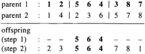
5.2.2. Order crossover (OX)

(Oliver et al. [47], Goldberg [20])

This crossover operator extends the modified crossover of Davis by allowing

two cut points to be randomly chosen on the parent chromosomes. In order to create

an offspring, the string between the two cut points in the first parent is first copied

to the offspring. Then, the remaining positions are filled by considering the sequence

of cities in the second parent, starting after the second cut point (when the end of

the c h r o m o s o m e is reached, the sequence continues at position 1).

354

J.-Y. Potvin, The traveling salesman problem

parent 1

:

parent 2

:

offspring

(step

1)

:

5 6 4

(step 2)

: 2 3

5 6 4

7 8 1

Figure 11. The order crossover.

by considering the corresponding sequence of cities in parent 2, namely 57814236

(step 2). Hence, city 5 is first considered to occupy position 6, but it is discarded

because it is already included in the offspring. City 7 is the next city to be considered,

and it is inserted at position 6. Then, city 8 is inserted at position 7, city 1 is inserted

at position 8, city 4 is discarded, city 2 is inserted at position 1, city 3 is inserted at

position 2, and city 6 is discarded.

Clearly, OX tries to preserve the relative order of the cities in parent 2, rather

than their absolute position. In figure 11, the offspring does not preserve the position

of any city in parent 2. However, city 7 still appears before city 8 and city 2 before

city 3 in the resulting offspring. It is worth noting that a variant of OX, known as

the maximal preservative crossover, is also described in [21].

5.2.3. Order-based crossover (OBX)

(Syswerda [58])

This crossover also focuses on the relative order of the cities on the parent

chromosomes. First, a subset of cities is selected in the first parent. In the offspring,

these cities appear in the same order as in the first parent, but at positions taken from

the second parent. Then, the remaining positions are filled with the cities of the

second parent.

In figure 12, cities 5, 4 and 3 are first selected in parent I, and must appear

in this order in the offspring. Actually, these cities occupy positions 2, 4 and 6 in

parent 2. Hence, cities 5, 4 and 3 occupy positions 2, 4 and 6, respectively, in the

offspring. The remaining positions are filled with the cities found in parent 2.

parent 1 :

parent 2 : 1 4 2 3 6 5 7 8

offspring : 1 5 2 4 6 3 7 8

Figure 12. The order-based crossover.

5.2.4. Position-based crossover (PBX)

(Syswerda [58])

The name of this operator is a little bit misleading, because it is the relative order of the cities that is inherited from the parents (the absolute position of the cities inherited from the second parent is rarely preserved). This operator can be seen as an extension of the order crossover OX, where the cities inherited from the first parent do not necessarily occupy consecutive positions.

In figure 13, positions 3, 5 and 6 are first selected in parent 1. Cities 5, 4 and 3 are found at these positions, and occupy the same positions in the offspring. The other positions are filled one by one, starting at position 1, by inserting the remaining cities according to their relative order in parent 2, namely 12678.

parent 1 : 1 2 _5 6 4 3 8 7

parent 2 : 1 4 2 3 6 5 7 8

offspring : 1 2 5 6 4 3 7 8

Figure 13. The position-based crossover.

5.2.5. Computational results

Studies by Oliver et al. [47] and Starkweather et al. [55] demonstrated that order-preserving crossover operators were clearly superior to the operators preserving the absolute position of the cities.

In [47], PMX, CX and OX were applied to the 30-city problem of Hopfield and Tank [28]. They found that the best tour generated with OX was 11% shorter than the best PMX tour, and 15% shorter than the best CX tour. In a later study [55], six different crossover operators were tested on the same problem [28]. Thirty different runs were performed with each operator. In this experiment, OX found the optimum 25 times (out of 30), while PMX found the optimum only once, and CX never found the optimum.

Table 1

Comparison of six crossover operators (30 runs) in [55].

Crossover No. of trials Pop. size Optimum Ave. tour length

Edge recombination (ER) 30,000 1,000 30/30 420.0

Order (OX) 100,000 1,000 25/30 420.7

Order based (OBX) 100,000 1,000 18/30 421.4

Position based (PBX) 120,000 1,000 18/30 423.4

Partially mapped (PMX) 120,000 1,400 1/30 452.8

Cycle (CX) 140,000 1,500 0/30 490.3

356

J.-Y Potvin, The traveling salesman problem

best possible results. Accordingly, the population size and number of trials (i.e., total

number of tours generated) are not the same in each case. The edge recombination

operator ER will be introduced in the next section, and should be ignored for now.

6.

The adjacency representation

The adjacency representation is designed to facilitate the manipulation of edges.

The crossover operators based on this representation generate offspring that inherit

most of their edges from the parent chromosomes.

The adjacency representation can be described as follows: city j occupies

position i in the c h r o m o s o m e if there is an edge from city i to city j in the tour. For

example, the c h r o m o s o m e 38526417 encodes the tour 13564287. City 3 occupies

position 1 in the c h r o m o s o m e because edge (1, 3) is in the tour. Similarly, city 8

occupies position 2 because edge (2, 8) is in the tour, etc. As opposed to the path

representation, a tour has only two different adjacency representations for symmetric

TSPs.

Various crossover operators are designed to manipulate this representation, and

are introduced in the next sections. These operators are aimed at transferring as many

edges as possible from the parents to the offspring. However, it is important to note

that they share a c o m m o n weakness: the selection of the last edge, that connects the

final city to the initial city, is not enforced. In other words, the last edge is added

to the final solution, without any reference to the parents. Accordingly, this edge is

rarely inherited.

6.1. ALTERNATE EDGES CROSSOVER ( G r e f e n s t e t t e et al. [22])

This operator is mainly of historical interest. As reported in [22], the results

with the operator have been uniformly discouraging. However, it is a good introduction

to the other edge-preserving operators.

Here, a starting edge

(i,j)

is selected at random in one parent. Then, the tour

is extended by selecting the edge (j, k) in the other parent. The tour is progressively

extended in this way by alternatively selecting edges from the two parents. When an

edge introduces a cycle, the new edge is selected at random (and is not inherited from

the parents).

parent 1 : 3 8 5 2 6 4 1 7

parent 2 : 4 3 6 2 7 5 8

1

offspring : 4 3 5 2 7 8 6

1

Figure 14. The alternate edges crossover.

representation. Here, edge (1, 4) is first selected in parent 2, and city 4 in position I

of parent 2 is copied at the same position in the offspring.

Then, the edges (4, 2) in parent 1, (2, 3) in parent 2, (3, 5) in parent 1 and (5, 7)

in parent 2 are selected and inserted in the offspring. Then, edge (7, 1) is selected

in parent 1. However, this edge introduces a cycle, and a new edge leading to a city

not yet visited is selected at random. Let us assume that (7, 6) is chosen. Then, edge

(6, 5) is selected in parent 2, but it also introduces a cycle. At this point, (6, 8) is

the only selection that does not introduce a cycle. Finally, the tour is completed with

edge (8, 1).

The final offspring encodes the tour 14235768, and all edges in the offspring

are inherited from the parents, apart from the edges (7, 6) and (6, 8).

In the above description, an implicit orientation of the parent tours is assumed.

For symmetric problems, the two edges that are incident to a given city can be

considered. In the above example, when we get to city 7 and select the next edge in

parent 1, edges (7, 1) and (7, 8) can both be considered. Since (7, 1) introduces a

cycle, edge (7, 8) is selected. Finally, edges (8, 6) and (6, 1) complete the tour.

parent 1 : 3 8 5 2 6 4 1 7

parent 2 : 4 3 6 2 7 5 8 1

offspring : 4 3 5 2 7

I 8 6

Figure 15. The alternate edges crossover (revisited).

6.2.

EDGE RECOMBINATION CROSSOVER (ER) (Whitley et al. [67])

Quite often, the alternate edge operator introduces many random edges in the

offspring, particularly the last edges, when the choices for extending the tour are

limited. Since the offspring must inherit as many edges as possible from the parents,

the introduction of random edges should be minimized. The edge recombination

operator reduces the myopic behavior of the alternate edge approach with a special

data structure called the "edge map".

Basically, the edge map maintains the list of edges that are incident to each

city in the parent tours and that lead to cities not yet included in the offspring. Hence,

these edges are still available for extending the tour and are said to be active. The

strategy is to extend the tour by selecting the edge that leads to the city with the

m i n i m u m number of active edges. In the case of equality between two or more cities,

one of these cities is selected at random. With this strategy, the approach is less likely

to get trapped in a "dead end", namely, a city with no remaining active edges (thus

requiring the selection of a random edge).

358

J.-Y. Potvin, The traveling salesman problem

1 has edges to : 3 4 7 2 has edges to : 3 4 8 3 has edges to : 1 2 5 4 has edges to : 1 2 6 5 has edges to : 3 6 7 6 has edges to : 3 4 5 7 has edges to : 1 5 8 8 has edges to : 1 2 7

Figure 16. The edge map.

(a)

City I is selected

city 2 has edges to : 3 4 8 city 3 has edges to : 2 5 6 city 4 has edges to : 2 6 city 5 has edges to : 3 6 7 city 6 has edges to : 3 4 5 city 7 has edges to : 5 8 city _8 has edges to : 2 7

(b)

City 8 is selected

city 2 has edges to : 3 4 city 3 has edges to : 2 5 6 city 4 has edges to : 2 6 city 5 has edges to : 3 6 7 city 6 has edges to : 3 4 5 city 7 has edges to : 5

(c)

City 7 is selected

city 2 has edges to : 3 4 city 3 has edges to : 2 5 6 city 4 has edges to : 2 6 city 5 has edges to : 3 6 city 6 has edges to : 3 4 5

(d)

City 5 is selected

city 2 has edges to : 3 4 city 3 has edges to : 2 6 city 4 has edges to : 2 6 city 6 has edges to : 3 4

(e)

City 6 is selected

city 2 has edges to : 3 4 city 3 has edges to : 2 city 4 has edges to : 2

(f)

City 4 is selected

city 2 has edges to : 3 city 3 has edges to : 2 6

(g)

City 2 is selected City 3 is selected

city 3 has edges to :

Figure 17. Evolution of the edge map.

Let us assume that city 1 is selected as the starting city. Accordingly, all edges

incident to city 1 must first be deleted from the initial edge map. From city 1, we

can go to cities 3, 4, 7 or 8. City 3 has three active edges, while cities 4, 7 and 8

have two active edges, as shown by edge map (a) in figure 17. Hence, a random

choice is made between cities 4, 7 and 8. We assume that city 8 is selected. From

8, we can go to cities 2 and 7. As indicated in edge map (b), city 2 has two active

edges and city 7 only one, so the latter is selected. From city 7, there is no choice

but to go to city 5. From this point, edge map (d) offers a choice between cities 3

and 6 with two active edges. Let us assume that city 6 is randomly selected. From

city 6, we can go to cities 3 and 4, and edge map (e) indicates that both cities have

one active edge. We assume that city 4 is randomly selected. Finally, from city 4 we

can only go to city 2, and from city 2 we must go to city 3. The final tour is 18756423

and all edges are inherited from both parents.

A variant which focuses on edges common to both parents is also described

in [55]. The common edges are marked with an asterisk in the edge map, and are

always selected first (even if they do not lead to the city with the minimum number

of active edges). In the previous example, (2, 4), (5, 6) and (7, 8) are found in both

parents and have priority over all other active edges. In the above example, the new

approach generates the same tour, because the common edges always lead to the

cities with the minimum number of active edges.

6.3.

HEURISTIC CROSSOVER (HX) [Grefenstette et al. [22], Grefenstette [23])

It is worth noting that the previous crossover operators did not exploit the

distances between the cities (i.e., the length of the edges). In fact, it is a characteristic

of the genetic approach to avoid any heuristic information about a specific application

domain, apart from the overall evaluation or fitness of each chromosome. This

characteristic explains the robustness of the genetic search and its wide applicability.

However, some researchers departed from this line of thinking and introduced

domain-dependent heuristics into the genetic search to create "hybrid" genetic algorithms.

They have sacrificed robustness over a wide class of problems for better performance

on a specific problem. The heuristic crossover HX is an example of this approach

and can be described as follows:

Step 1.

Step 2.

Step 3.

Step 4.

Choose a random starting city from one of the two parents.

Compare the edges leaving the current city in both parents and select the

shorter edge.

If the shorter parental edge introduces a cycle in the partial tour, then extend

the tour with a random edge that does not introduce a cycle.

360

J.-Y. Potvin, The traveling salesman problem

Note that a variant is proposed in [36,56] to emphasize the inheritance of

edges from the parents. Basically, step 3 is modified as follows:

Step 3'. If the shorter parental edge introduces a cycle, then try the other parental

edge. If it also introduces a cycle, then extend the tour with a random edge

that does not introduce a cycle.

Jog et al. [29] also proposed to replace the random edge selection by the

selection of the shortest edge in a pool of random edges (the size of the pool being

a parameter of the algorithm).

6.4. COMPUTATIONAL RESULTS

Results reported in the literature show that the edge-preserving operators are

superior to the other types of crossover operators (Liepins et al. [37], Starkweather

et al. [55]). In particular, the edge recombination ER outperformed all other tested

operators in the study of Starkweather et al. [55]. A genetic algorithm based on ER

was run 30 times on the 30-city problem described in [28], and the optimal tour was

found on each run (see table 1).

However, these operators alone cannot routinely find good solutions to larger

TSPs. For example, Grefenstette et al. [22] applied the heuristic crossover HX to

three TSPs of size 50, 100 and 200, and the reported solutions were as far as 25%,

16% and 27% over the optimum, respectively. Generally speaking, many edge crossings

can still be observed in the solutions generated by the edge-preserving operators.

Accordingly, powerful mutation operators based on k-opt exchanges (Lin [38]) are

added to these operators to improve solution quality. These hybrid schemes will be

discussed in the next section.

Table 2 summarizes sections 4 to 6 by providing a global view of the various

crossover operators for the TSP. They are classified according to the type of information

transferred to the offspring (i.e., relative order of the cities, absolute position of the

cities, or edges).

Table 2

Information inheritance for nine crossover operators.

Crossover operator Relative order Position Edge Modified

Order (OX) Order based (OBX) Position based (PBX) Partially mapped (PMX) Cycle (CX)

Alternate edge

Edge recombination (ER) Heuristic (HX)

X X X X

As a final remark, it is worth noting that Fox and McMahon [13] describe an

alternative matrix-based encoding of the TSP tours. Boolean matrices, encoding the

predecessor and successor relationships in the tour, are manipulated by special union

and intersection crossover operators. This approach provided mixed results on problems

with four different topologies. In particular, union and intersection operators were

both outperformed by simple unary mutation operators. However, these operators

presented an interesting characteristic: they managed to make progress even when

elitism was not used (i.e., when the best tour in a given population was not preserved

in the next population).

Recently, Homaifar et al. [27] reported good results with another matrix-based

encoding of the tours. In this work, each chromosome corresponds to the adjacency

matrix of a tour (i.e., the entry (i,j) in the matrix is 1 if arc

(i,j)

is in the tour).

Accordingly, there is exactly one entry equal to 1 in each row and column of the

matrix. Then, the parent chromosomes produce offspring by exchanging columns via

a specialized matrix-based crossover operator called MX. Since the resulting off-

spring can have rows with either no entry or many entries equal to 1, a final "repair."

operator is applied to generate valid adjacency matrices. A 2-opt exchange heuristic

is also used to locally optimize the solutions. With this approach, the authors solved

eight classical TSP problems ranging in size from 25 to 318 nodes, and they matched

the best known solutions for five problems out of eight.

7.

Mutation operators

Mutation operators for the TSP are aimed at randomly generating new

permutations of the cities. As opposed to the classical mutation operator, which

introduces small perturbations into the chromosome, the permutation operators for

the TSP often greatly modifies the original tour. These operators are summarized

below.

7.1. SWAP

Two cities are randomly selected and swapped (i.e., their positions are ex-

changed). This mutation operator is the closest in philosophy to the original mutation

operator, because it only slightly modifies the original tour.

7.2. L O C A L H I L L - C L I M B I N G

362 J.-Y. Port, in, The traveling salesman problem

7.3. SCRAMBLE

Two cut points are selected at random on the chromosome, and the cities within the two cut points are randomly permuted.

7.4. COMPUTATIONAL RESULTS

The studies of Suh and Gucht [56], Jog et al. [29], and Ulder et al. [64] pointed out the importance of the hill-climbing mutation operators. Suh and Gucht added a 2-opt hill-climbing mutation operator to the heuristic crossover HX. On the first 100- city problem in [33], they found a tour of length 21,651, only 1.7% over the optimum. The heuristic crossover HX alone found a solution as far as 25% over the optimum. On the same problem, Jog et al. [29] found that the average and best tours, over 10 different runs, were 2.6% and 0.8% over the optimum using a similar approach based on HX and 2-opt. By adding Or-opt (i.e., some chromosomes perform a 2-opt hill-climbing, while others perform an Or-opt), the average and best solutions improved to 1.4% and 0.01% over the optimum, respectively.

In [64], eight classical TSPs ranging in size from 48 to 666 cities were solved with a genetic algorithm based on the order crossover OX and the L i n - K e r n i g h a n hill-climbing heuristic. Five runs were performed on each problem and the averages were within 0.4% of the optimum in each case. Table 3 shows their results for the three largest problems of size 442, 532 and 666 (Padberg and Rinaldi [49], Gr6tschel and Holland [24]). This genetic algorithm was compared with four other solution

Table 3

Average percent over the optimum (5 runs) for five solution procedures in [64].

CPU time SA M - 2 o p t M - L K G - 2 o p t G - L K TSP

(seconds) (%) (%) (%) (%) (%)

442-city 4,100 2.60 9.29 0.27 3.02 0.19 532-city 8,600 2.77 8.34 0.37 2.99 0.17 666-city 17,000 2.19 8.67 1.18 3.45 0.36

SA simulated annealing.

M-2opt Multi-start 2-opt (a new starting point is chosen when a local optimum is found).

M-LK Multi-start Lin-Kernighan.

G-2opt Genetic algorithm with 2-opt mutation operator.

G-LK Genetic algorithm with Lin-Kernighan mutation operator.

Braun [7] also reported interesting results on the 442- and 666-city problems.

Fifty different runs were performed with a genetic algorithm based on the order

crossover OX and a mixed 2-opt, Or-opt hill-climbing. He found the optimum of the

442-city problem, and a solution within 0.04% of the optimum for the 666-city

problem. On a 431-city problem, each run generated a solution within 0.5% of the

optimum, and about 25% of the solutions were optimal. In the latter case, the average

run time on a Sun workstation was about 30 minutes. Braun also reported that a 229-

city problem was solved in less than three minutes.

8.

Parallel implementations

The genetic algorithm is well suited for parallel implementations, because it

is applied to a population of solutions. In particular, a parallel implementation described

in [ 2 1 , 4 3 - 4 5 ] was very successful on some large TSPs.

In this implementation, each processor handles a single chromosome. Since the

processors (chromosomes) are linked together according to a fixed topology, the

population of chromosomes is structured. Namely, a neighborhood can be established

around each chromosome based on this topology, and reproduction takes place among

neighboring chromosomes only. Since the neighborhoods intersect, the new genetic

material slowly "diffuses" through the whole population. One main benefit of this

organization over a uniform population, where each chromosome can mate with any

other chromosome, is that diversity is more easily maintained in the population.

Accordingly, the parallel genetic algorithm can work with smaller populations without

suffering from premature convergence.

The parallel genetic algorithm can be described as follows.

Step 1.

Step 2.

Step 3.

Step 4.

Step 5.

Create an initial random population.

Each chromosome performs a local hill-climbing (2-opt).

Each chromosome selects a partner for mating in its neighborhood.

An offspring is created with an appropriate crossover operator (OX).

The offspring performs a local hill-climbing (2-opt). Then, it replaces its

parent if the two conditions below are satisfied:

(a) it is better than the worst chromosome in the parent's neighborhood;

(b) it is better than the parent, if the parent is the best chromosome in its

neighborhood (elitist strategy).

364 J.-Y Potvin, The traveling salesman problem

local optima. In particular, it combines two local optima to generate a new local

optimum that is hopefully better than the two previous ones.

In [68], the authors describe an alternative implementation where subpopulations

of chromosomes evolve in parallel on different processors. After a fixed number of

iterations (based on the size of the subpopulations), the best chromosomes on each

processor migrate to a neighboring processor and replace the worst chromosomes on

that processor. A similar idea is also found in [7].

8.1. COMPUTATIONAL RESULTS

Whitley et al. [68] solved a 105-city problem with their distributed approach

based on migration using the edge recombination operator ER for crossover and no

mutation operator. With this parallel algorithm, they found the optimum tour in 15

different runs (out of 30). In addition, 29 solutions were within 0.5% of the optimum,

and all solutions were within 1% of the optimum.

The parallel genetic algorithm [21,44] was applied to the classical 442- and

532-city problems described in [24,49]. On a parallel computer with 64 T800

transputers, this algorithm solved the two problems in approximately 0.6 and one

hour, respectively (the computation times can change depending on the parameter

settings). The best solutions for the 442- and 666-city problems were within 0.3%

and 0.1% of the optimum, respectively. Note that Braun [7] found the optimal solution

of the 442-city problem with his approach (cf. section 7).

9.

Overview of the computational results

The results published in the literature on genetic algorithms cannot be easily

compared, because various algorithmic designs and parameter settings are used. With

respect to the algorithmic design, most implementations use a proportional selection

scheme based on some transformation of the raw fitness value or tour length (cf.

scaling, ranking, etc.). Various generation replacement mechanisms are also described,

ranging from a complete replacement of the population without any form of elitism,

to the replacement of the worst tour by a single newly created tour. Judicious parameter

settings can also improve the quality of the final solution (e.g., population size,

maximum number of generations, crossover and mutation rates, etc.). Finally, the

initial population can be generated in various ways (e.g., random tours versus heuristic

tours).