The Mixed Finite Element Multigrid Preconditioned
MINRES Method for Stokes Equations
K. Muzhinji
1, S. Shateyi
1†and S, S. Motsa
21 University of Venda, Department of Mathematics,P Bag X5050, Thohoyandou 0950, South Africa 2 University of KwaZulu-Natal, Department of Mathematics, P Bag X01, Pietermaritzburg, Scottsville 3209,
South Africa
†Corresponding Author Email:[email protected]
(Received March 2, 2014; accepted March 16, 2015)
ABSTRACT
The study considers the saddle point problem arising from the mixed finite element discretization of the steady state Stokes equations. The saddle point problem is an indefinite system of linear equations, a feature that degrades the performance of any iterative solver. The heart of the study is the construction of fast, robust and effective iterative solution methods for such systems. Specific attention is given to the preconditioned MINRES solver PMINRES which is carefully treated for the solution of the Stokes equations. The study concentrates on the block preconditioner applied to the MINRES to effectively solve the whole coupled system. We combine iterative techniques with the MINRES as preconditioner approximations to produce an efficient solver for indefinite system of equations. We consider different preconditioner approximations of the building blocks of the preconditioner and compare their effects in accelerating the MINRES iterative scheme. We give a detailed overview of the algorithmic aspects and the theoretical convergence analysis of our solver. We study the MINRES method with the following preconditioner approximations: diago-nal, multigrid v-cycle, preconditioned conjugate gradient and Chebyshev semi iteration methods. A comparative analysis of the preconditioner approximations show that the multigrid method is a suit-able accelerator for the MINRES method. The application of the preconditioner becomes mandatory as evidenced by poor performance of the MINRES as compared to PMINRES. We study the prob-lem in a two dimensional setting using the Hood-TaylorQ2−Q1stable pair of finite elements. The incompressible flow iterative solution software(IFISS) matlab toolbox is used to assemble the ma-trices. We present the numerical results to illustrate the efficiency and robustness of the MINRES scheme with the multigrid preconditioner.
Keywords: Stokes equations; Mixed finite element method; Block preconditioner; Preconditioned
MINRES method(PMINRES)
NOMENCLATURE
ˆ
A preconditioner for matrix A
(A= (ai j)i,j, ...) matrices
h,l mesh size and mesh level ˆ
S preconditioners matrix S
c
M
A preconditioner approximation for ˆAc
M
S preconditioner approximation for ˆS(u, ..) vector valued functions u·v scalar product
Vh,Wh finite element spaces
(p,q, ...) s scalar values
R
2 space of dimension 2Ω∈
R
2 solution domain∂Ω boundary ofΩ
∇u:∇v componentwise scalar product
∇p gradient ofp
∆u Laplacian ofu div u divergence ofu
α,α1 continuity constants
α0 coercivity constant
β continuous inf-sup constant
β1 discrete inf-sup constant
η global error estimator
k∇·ukΩ velocity divergence error L2(Ω) Lebesgue space of measurable
functions f
H1(Ω),H01(Ω) Sobolev spaces
Q2−Q1 biquadratic-bilinear finite eigenvalue elements
λ,[ω,ω¯],[δ,δ¯] eigenvalues and bounds
1. INTRODUCTION
In this paper we analyze the performance of the MINRES and the preconditioned MINRES method on the numerical solution of the steady state Stokes equations. We study Stokes equa-tions which govern the flow of steady, viscous, incompressible, isothermal, Newtonian fluids. They arise by simplifying the incompressible Navier-Stokes equations through the omission of the convective derivative and setting the time derivative to zero. For more details on the derivation, we refer to (Bramble and Pasciak 1999; Brenner and Scott 2008; Brezinski 2005; Cebeciet al.2005; Elmanet al.2005; Ferziger and Peric 2002; Shaughnessyet al.2005; Tuet al. 2008; Zulehner 2002). This results in the following system of linear system partial differ-ential equation:
−△u+∇p = f in Ω (1)
divu = 0 in Ω (2)
u = 0 on ∂Ω (3)
whereΩ is assumed to be a bounded open set in
R
2, with a sufficiently smooth and Lipschitz continuous boundary∂Ω,f:Ω→R
is a density of body forces acting on the fluid(e.g gravita-tional force) and the kinetic viscocity of the fluid has been set to 1. The problem is to find the vector functionu:Ω→R
2which denotes the velocity of the fluid andp:Ω→R
pressure.The solution procedure begins with the mixed finite element discretization of the domain of the Stokes equations Eqs.(1)-(3) which results in a coupled linear algebraic systems of block structure. This study employs the Hood-Taylor Q2−Q1 pair of finite elements as used in El-man (2007). The efficient iterative techniques for solving the linear algebraic system of the saddle point form Eq.(4) below are considered. The block coupled system has the form
A BT
B O
u p
=
f g
(4)
with A- an n×n symmetric positive definite 2×2 block matrix, B- an m×n matrix with
full rank and m≤n, and that the coefficient matrix
M
is an(n+m)×(n+m) symmetric indefinite matrix, hence MINRES is applicable as a solution iterative scheme Paige and Saun-ders (1975). If these conditions on the matri-ces A and B above hold then the invertibility of the coefficient matrixM
is guaranteed and that the Schur compliment formSis also sym-metric positive definite (Elmanet al. 2005; El-man and Golub 1994; Reusken and Gross 2011; Zulehner 2000; Zulehner 2002). Since matrixM
is very large, sparse and indefinite well es-tablished iterative schemes such as Krylov sub-space methods become very slow, stagnant or fail to converge if not conveniently precondi-tioned. The choice of the preconditioner is such that the preconditioned matrix satisfies prop-erties needed for the numerical scheme. For the MINRES it means that the preconditioner should be symmetric and positive definite to preserve the symmetry of the preconditioned system. Preconditioning enhances the conver-gence behavior of the iterative schemes. There are a number of solution schemes for finding the solution (u,p) of Eq. (4) and provided the pre-conditioners for A and S are at available. A va-riety of preconditioned iterative schemes exist to tackle the system. The different variants of preconditioners were developed thereafter. This study analyses the performance and the theo-retical behaviour of preconditioning strategies and preconditioner approximations used with Krylov subspace iteration to obtain the solution of the system Eq. (4). For this class of systems, special iterative schemes must be designed be-cause of their indefiniteness and poor spectral properties. A very extensive survey of these schemes is given in (Benziet al. 2005; Elman et al. 1999; Turek 1999) among others. Some recent studies on the numerical solution of such system includes (Herzog and Sachs 2005; Pe-ters et al. 2005; Rehman and Vuik 2007; Stoll and Wathen 2008; Vuik 1996;?; Zulehner 2000; Zulehner 2002). The candidate method of choice for symmetric indefinite system is the MINRES introduced in Paige and Saunders (1975) as a method of minimizing the residualap-ply the MINRES method we need the precon-ditioner to be symmetric and positive definite and hence the block diagonal preconditioners would present the natural choice Elmanet al. (1999). In this paper we apply the MINRES scheme with a block diagonal preconditioner
c
M
= bA OO Sb
withAband Sbthe preconditioner of the (1,1)-A block and the Schur compliment respectively. The PMINRES and its variants has been in-vestigated in (Elman et al. 2005; Larin and Reusken 2008; Peters et al. 2005; Rees and Stoll 2010; Stoll and Wathen 2008; Wathen and Rees 2009). This study is influenced by the work by (Elman et al. 1999; Rees and Stoll 2010; Stoll and Wathen 2008) and the variant of the method considered in this study is the one implemented as a driver in matlab.
In this study the velocity is preconditioned by applying multigrid v-cycle method and for the pressure, its preconditioner is an iterative solver using the pressure mass matrix. The main point of this preconditioner is to reduce the low frequency error component on a coarser grid, which the high frequency components of error are reduced by a smoother on a fine grid. The multigrid method has been studied in (Bren-ner and Scott 2008; Hackbucsh 1985; Wessel-ing 1999). The multigrid are the most effective methods for solving large linear systems aris-ing from the elliptic partial differential equa-tions. The philosophy of the multigrid is based on the combination of two key principles. The first is that the high frequency components of the error are reduced by applying the basic it-erative solvers like Jacobi or Gauss Seidel as smoothers. Next, the low frequency errors are reduced by coarse grid correction procedure. The smooth error components are represented as a solution of an approximate coarser system. After solving the coarser problem, the solution is interpolated back to correct the fine grid ap-proximation for its low frequency errors. The way the multigrid components are linked that is smoothing, restriction, prolongation and the error of the coarse grid is illustrated in the algo-rithm below.
Algorithm 1. Solve Ahuh=bhwhere the
sub-script is used for fine grid and H for coarse rid.
• Perform smoothing by using k1iterations of an iterative method (Jacobi, Gauss-Seidel etc) on the problem Ahuh=bh
• Compute the residual rh=bh−Ahuh
• Solve for the coarse grid correction AHeH=bH
• Prolongate and update uh=uh+PeH
• Perform smoothing by using k2iterations of an iterative method (Jacobi, Gauss-Seidel etc) on the problem Ahuh=bh
The algorithm is a two grid method but step 4 can be utilised in various ways. The classical method of solving it employs recursive calls to the two grid method. If the recursion is carried out in a loop, allowing different numbers of it-erative sweeps on different coarse grids, we ob-tain v-cycle, w-cycle and f-cycle. In this study we use the multigrid v-cycle with Gauss-Seidel smoother as preconditioner approximation for both A and S.
The rest of the paper is organized as follows. In section 2 the discrete system of the Stokes equations discretized by mixed finite element method is discussed. In section 3 the iterative solution technique: The MINRES algorithm and the PMINRES algorithm together with the block preconditioner are outlined. The method relies on good approximations to the (1,1)-block and Schur complement. We also discuss the suitable bounds and the known theoretical con-vergence analysis based on the eigenvalue prob-lem and results. In the final section 4 a numer-ical experimental results and comparative anal-ysis on the effectiveness of the preconditioner approximations are presented, discussed and the conclusion given in section 5.
2. THE DISCRETE STOKES EQUA-TIONS
For the discretization of the Stokes equations we need to transform the system Eqs. (1)-(3) firstly to the variational form. The varia-tional formulation of the Stokes equations re-quires that we define the following solution and test spaces:
H1(Ω):={u:Ω−→
R
|u, ∇u∈L2(Ω)} H10(Ω):={v: v∈H1(Ω)|v=0on∂Ω}. By multiplication of the first Eq. (1) withv∈ H01(Ω)
Find u∈H01(Ω) and p∈L2(Ω) such that:
a(u,v)−b(v,p) =F(v) ∀v∈H01(Ω) (5)
b(u,q) =0 ∀q∈L2(Ω). (6)
where a(.,.) and b(.,.) are continuous bilinear forms defined as
a(u,v) =
Z
Ω∇
u:∇vdx (7)
b(u,q) =
Z
Ω(
divv)qdx (8)
F(v) =
Z
Ωf·vdx (9)
where ∇u : ∇v represents a componentwise scalar product that is∇ux·∇vx+∇uy·∇vyand a:H01(Ω)×H01(Ω)−→
R
andb:H01(Ω)×L2(Ω) −→
R
. The well-posedness follows from the coercivity of a(.,.) in the Lax-Milgram theorem (Ciarlet (1978), Gockenbach (2006)) and partly from the inf-sup condition (Braess (2007), Brenner and Scott (2008), Elakkad et al. (2010), Elman et al. (2005), Girault and Raviart (1986), Gunzburger (1989)). Below is a sketch of the analysis of the existence unique-ness and stability of the solution(u,p)∈V×W of mixed problem Eqs. (5) and (6) withV=H01 and W =L2(Ω):
i. the bilinear form a(.,.) is bounded or con-tinuous:
|a(u,v)|≤αkukV· k vkV for allu,v∈Vandα∈
R
ii. the bilinear form a(.,.) is coercive on V:=H01(Ω) that is there exists a pos-itive constant α0 : a(v,v) ≥ α0 k vk2
V f or all v∈V.
iii. the bilinear a(.,.) is symmetric and non-negative
a(u,v) = a(v,u) and a(v,v)≥0 f or allu,v∈V
iv. the bilinear form b(.,.) is bounded:
|b(u,q)|≤α1kukV· k qkW for allu∈V,q∈W andα1∈
R
v. the bilinear form b(.,.) satisfies the inf-sup condition, that is:
there exists a constant β:
inf 06=q∈W06=supv∈V
|b(v,q)| kvkV· kqkW ≥
β>0
For instance in Girault and Raviart (1986) it is shown that in our concrete case b(.,.) fulfills the inf-sup condition, thus we can combine the as-sumptions above to give the following theorem
Theorem 2. Variational problem Eqs. (5) and
(6) is uniquely solvable provide properties (i)-(v) are all satisfied.
The details of the proof can be found in (Girault and Raviart 1986; Brezinski 2005).
2.1 The Mixed Finite Element
Discretiza-tion
The mixed finite element discretization of the variational formulation of the Stokes equations results in a linear algebraic system of equations. The finite element method described here is based on the references (Braess 2007; Brenner and Scott 2008; Ciarlet 1978; Donea and Huerta 2003; A. Elakkad and A. Elkhalfi and N. Gues-sous 2010; Gunzburger 1989). We will intro-duce the concept of mixed finite element meth-ods. Details can be found in (Brenner and Scott 2008; Ciarlet 1978; Donea and Huerta 2003; A. Elakkad and A. Elkhalfi and N. Guessous 2010; Gockenbach 2006).
We assume thatΩ⊆
R
2. We define the follow-ing finite dimensional spaces .LetWh andVhbe subspaces of W andV re-spectively and now we can formulate a discrete version of problem Eqs. (5) and (6):
Find a couple(uh,ph)∈Vh×Whsuch that
a(uh,vh)−b(vh,ph) =F(vh), ∀vh∈Vh (10)
b(uh,qh) =0, ∀qh∈Wh. (11)
The finite element discretization should satisfy the discrete inf-sup condition. The following theorem shows that again the inf-sup condition is of major importance.
Theorem 3. Assume that a is Vh-elliptic
(with h independent ellipticity constant) and that there exists a constantβ>0(independent of h) such that the discrete inf-sup condition
inf 06=qh∈Wh
sup 06=vh∈Vh
|b(vh,qh)|
kvhkVhkqhkWh
holds. Then the associated (discretized, steady state) Stokes problem has a unique solution
(uh;ph), and there exists a constantβ1such that
ku−uhkV+kp−phkW ≤β1(inf
v∈Vhk
u−uhkV) + ( inf
q∈Wh
kp−phkW). (13)
(for the proof we refer to Girault and Raviart (1986)).
If the basis ofWhis given by {ψ1, ...,ψm} and of Vhbe given by {ϕ1, ...,ϕn} then
uh= ni
∑
i=1 ui·ϕi+
ni+n∂
∑
i=ni+1
ui·ϕi, (14)
ph= m
∑
k=1
pkψk. (15)
where ni is the number of inner nodes, n∂ is
the number of boundary nodes so the coeffi-cientsui:i=ni+1, ..,ni+n∂ interpolates the
boundary data andn=ni+n∂. The mixed
fi-nite element entails partitioning of the solution domain Ω into quadrilaterals, in our case that is Ω=∪iτi we denote a set of quadrilateral elements byTh={τ1,τ2,τ3, ...}and on each el-ementτiand we denote the spacePk(τi)of de-gree less than or equal to k. There are a vari-ety of finite element pairs whose effectiveness is through stabilization[14]. In this work we are going to use Hood-TaylorQ2−Q1 pair of quadrilateral finite elements which are known to be stable.
We specify
Vh:={uh∈V|uh|τi∈P2(τi),∀ elements τi}, Wh:={ph∈W|ph|τi∈P1(τi),∀ elementsτi},
An element(uh,ph)∈Wh×Vhis uniquely de-termined by specifying components of vector uh on the nodes and on the midpoints of the edges of the elements and the values of phon the nodes of the elements. The mixed finite el-ement method results in the coupled linear al-gebraic system of equations which has to be solved by the appropriate solvers. The resulting coupled system is
Ah BTh Bh O
uh ph
=
fh gh
(16)
withAh is a block Laplacian matrix andBhis the divergence matrix whose entries are given
by
A= [ai j], ai j= Z
Ω(∇φi:∇φj)i,j=1,...,n
B= [bki], bki=− Z
Ω(ψk∇·φi))k=1,...,m;i=1,...,n
The entries of the right hand side vector are
f= [fi], fi= Z
∂Ω
f·φi− n+n∂
∑
i=n+1 ui
Z
Ω(∇φi:∇φj)
g= [gk], gk= n+n∂
∑
i=n+1 ui
Z
Ω(ψk∇·φi))
The linear algebraic system can be represented as
M
x=b, (17)where
M
:=
Ah BTh Bh O
; x:=
uh ph
and
b:=
fh gh
.
The solution vectors(uh,ph)are the mixed fi-nite element weak solution. The system Eqs. (16)-(17) is called the discrete Stokes problem.
The discretization and assembling of matri-ces are done by the matlab implementation of the mixed finite element method (Elmanet al. 2005). Ahis stiffness matrix resulting from the discretization of the Laplacian. The resultant coefficient matrix is large, sparse, indefinite and the system must be solved iteratively, in this case by MINRES solvers. We are interested in the approximate solution of Eq. (16) at the finest mesh/discretization.
3. THE PRECONDITIONED MINRES
ITERATIVE SCHEME
In this section we outline the algorithmic struc-ture of the iterative scheme for solving the discretized linear algebraic system Eq. (16). The main goal is to find the approximate pair
following residual minimization problem:
Given the initial guess x0, determine xi ∈ x0+
K
i(M
;r0)such thatk
M
xi − b k= min(kM
xi − b k| x0 +K
i(M
;r0)) where r0 = b −
M
x0 andK
i(M
,r0) =spanr0,
M
r0,M
2r0, ...,M
i−1r0 is the Krylov subspace. Below is the MINRES algorithm for computing the iteratexi as given in (Elmanet al.(1999)).Algorithm 4. The MINRES Algorithm
v0=0, w0=0, w1=0 Choosex0, compute v1=b−
M
x0, set γ1=kv1k setη=γ1, s0=s1=0, c0=c1=1for i = 1,2...until convergence do vi=vi
γi δi=h
M
vi,vii vi+1=M
vi−δivi−γivi−1γi+1=kvi+1k
α0=ciδi−ci−1siγi
α1=
q
α2 0+γ2i+1
α2=siδi+ci−1ciγi
α3=si−1γi ci+1=α0α1, si+1=γα1i+1 wi+1=(
vi−α3wi+1−α2wj)
α1
xi=xi−1+ci+1ηwi+1
η=−si+1η Test for convergence
end for
We consider a symmetric positive definite block preconditioner
M
c ofM
as studied in (Schor-bel and Zulehner (2007), Zulehner (2002)). The block triangular preconditioner is given asc
M
:= bA OO Sb
(18)
Such that the left preconditioned system be-comes
c
M
−1M
x=M
c−1b (19) which isf
M
x=eb (20)The residual minimization criteria is applied to the preconditioned system Eq. (20):
Given the initial guess x0 ∈
R
n+m×n+m and initial residual er0 = eb−M
fx0, determine xi ∈ x0+K
i(M
f;er0) such that: kM
fxi−eb k= min(k
M
cxi−eb k | x0+K
i(M
f;er0)) where er0 =eb−M
fx0 andK
i(M
f,er0) = spanner0,M
fer0,M
f2er0, ...,M
fi−1er0o
is the
Krylov subspace andh·,·iMb=hMb·,·i.
Then the preconditioned residual
M
c−1(b−M
x)is minimized in k · kMb over transformed Krylov subspace. The implementation of the PMINRES requires one evaluation ofM
c−1zfor a given z and one multiplication by A per iter-ation. The evaluation of the preconditioner is achieved by solving a linear systemz=M
cy The PMINRES method is outlined in the algo-rithm below.Algorithm 5. The PMINRES Algorithm
v0=0, w0=0, w1=0 Choosex0, compute v1=b−
M
x0, set γ1=kv1k Solve Mz1b =v1 set γ1=p
hz1,v1i setη=γ1, s0=s1=0, c0=c1=1
for i = 1,2...until convergence do zi=zi
γi δi=h
M
zi,zii vi+1=M
vi−(δγii)vi−(γγii−1)vi−1
SolveMzib +1=vi+1
γ1=
p
hzi+1,vi+1i
α0=ciδi−ci−1siγi
α1=
q
α2 0+γ2i+1
α2=siδi+ci−1ciγi
α3=si−1γi ci+1=α0α1, si+1=γα1i+1 wi+1=(
zi−α3wi+1−α2wj)
α1
xi=xi−1+ci+1ηwi+1
η=−si+1η Test for convergence
end for
The main convergence results for PMINRES method are due to (Peters et al. 2005; Rees and Stoll 2010; Reusken and Gross 2011). The convergence analysis is based on the eigenvalue analysis of the preconditioned matrix system. The spectral analysis of the preconditioner in-fluences the convergence properties of the itera-tive scheme connected with the approximations of A andb S. We require that the eigenvaluesb of the preconditioned system are well clustered and distributed provided that the eigenvalues of
b
Theorem 6. Let
M
∈R
(n+m)×(n+m) besym-metric and Mb ∈
R
(n+m)×(n+m) be symmetricand positive definite. For xi, i>0computed in the preconditioned MINRES algorithm we de-fine bri=Mb−1(b−
M
xi). Then the following holdskbrikMb=minpi∈Pi;p0=1kpi(Mb−
1
M
)b
r0kMb ≤minpi∈Pi;p0=1maxλ∈σ(Mb−1M) |pi(λ)| kbr0kMb (21)
The maximum is over the eigenvalues λ of
c
M
−1M
.For the proof we refer to (Reusken and Gross (2011)). The theorem gives that the rate of convergence of the preconditioned MINRES method depends onσ(Mb−1
M
). We need to de-rive these bounds. The special case is when we have Ab=A and Sb=S and we have thatσ(Mb−1
M
)∈ {12(1−√
5),1,12(1+√5)}. This yields an exact solution in at most 3 iterations (Elmanet al.1999; Peterset al.2005; Reusken and Gross 2011). In our case this is not practi-cally feasible since the Schur complimentSb=
BAb−1BT is not computed explicitly since Ab−1 is not sparse anymore and is very costly to use since the matrix vector computation Szb =
B(Ab−1(BTz))that involves solving a linear sys-tem like Ayb =BTz. Since the exact precon-ditioning is not feasible, we use the precondi-tioner approximations
M
cAo f A andbM
cSo f S.b The quality of these approximations is mea-sured by using the spectral equivalences or in-equalities. In order to quantify the quality of the both approximations we use the spectral analy-sis under the following conditions. For the pre-conditioner approximationsM
cA andM
cS and letω, ω,δ,δ>0 such thatω≤λ= x
TAx xT
M
cAx
≤ω (22)
δ=x
TBA−1BTx
xT
M
cSx ≤δ (23)Using the results in (Elmanet al. 1999; Peters et al. 2005; Rees and Stoll 2010) we obtain the result for the eigenvalue bounds for the precon-ditioned matrix. The conditions Eqs. (22) and (23) implies that[ω,ω]contain all the eigenval-ues of the preconditioned matrix Ab−1A and δ
is the smallest eigenvalue ofSb−1S, with δ the
inf-sup constant. As a consequence the follow-ing theorem for eigenvalue bounds points to the convergence of PMINRES method.
Theorem 7. Let ω, ω, δ, δ>0 and assume
that Eqs. (22) and (23). Let (λ,
u p
)be an
eigenpair
M
f. Then following eigenvalue prob-lemM
u p
=λ
M
cA OO
M
cS!
u p
(24)
and A,S,MbA and MbS is positive definite. Then
λ is real and positive that satisfies
ω−√ω2−4(ωδ)
2 ≤λ≤
ω−√δ2+4δω
2
ω≤λ≤ω ω+√ω2+4ωδ
2 ≤λ≤
ω+√ω2+4(δω)
2
with ω, ω, δ, δ measures the qual-ity and effectiveness of the precondition-ers(approximations)MbA of A andMbSto S.
For the proof we refer to (Elman et al. 1999; Elmanet al.2005; Rees and Stoll 2010).
Remark 8. The results of the theorems (6) and
(7) indicate that as long as we choose the ap-proximations
M
cA andM
cS close enough to A and S then we can expect a good clustering of eigenvalues of the eigenvalue problem that is the spectral constants are ω, ω, δ, δ close 1 then one can expect a fast convergence of the PMINRES method.4. NUMERICAL RESULTS
In this section we present the numerical solu-tion of classical Stokes problem Eqs. (1)-(3) us-ing the solvers presented above. The solvers are denoted by MINRES (algorithm 4) and PMIN-RES (algorithm 5). We present the results of this method as outlined above to run the tradi-tional test problem, the driven cavity flow prob-lem (Brambleet al.1997; Bramble and Pasciak 1999; Elmanet al. 1999; Larin and Reusken 2008). It is a model of the flow in a square cav-ity (the domain isΩ ) with the top lid moving from left to right in our case the regularized cav-ity model{y=1 : −1≤x≤1|ux=1−x4} Elman et al. (1999). The Dirichlet no-slip boundary condition is applied on the side and bottom boundaries. The mixed finite element method was used to discretize the cavity domain
We pay particular attention to the computational performance of the MINRES and PMINRES methods at different grid levels. We compare the effectiveness of different approximations for the preconditioners
M
cAandM
cS. The following are considered, no preconditioning and different combinations of the preconditionersA andb Sbare considered as outlined in section 3:i. MINRES with no preconditioning
ii. PMINRES: diagonal preconditioning (diag(A), diag(Q)), Q is the pressure mass matrix.
iii. PMINRES: multigrid v-cycle with Gauss
Seidel smoothing for
M
cAand multigrid v-cycle for theM
cSusing the pressure mass matrix(Amg,Smg)iv. PMINRES: multigrid v-cycle with Gauss
Seidel smoothing for
M
cA and diagonally preconditioned standard conjugate gradi-ent for theM
cS using the pressure mass matrix(Amg,Spcg)v. PMINRES: multigrid v-cycle with Gauss Seidel smoothing for
M
cAand Chebyshev semi-iteration for theM
cSusing the pres-sure mass matrix?(Amg,Scheb).vi. PMINRES: multigrid v-cycle with Gauss
Seidel smoothing for
M
cA and diagonal preconditioning using the pressure mass matrix(Amg,diag(Q)).The comparison is made on the performance of the MINRES and PMINRES schemes with different combinations of preconditioners (i)-(vi) in terms of iterative counts and CPU time. The numerical treatment is given to the discrete Stokes problem which resulted from the mixed finite Hood-Taylor Q2-Q1 stable elements con-sisting of biquadratic elements for the velocities and bilinear elements for the pressure, on a uni-form grid. Implementation was peruni-formed on a windows 7 platform with 2.13 GHz speed intel dual core processor by using matlab 7.14 pro-gramming language. For the discretization we start with a uniform square grid withh0=12and we apply regular refinements to this starting dis-cretization.
The Fig. 2 show the snapshot of the error indi-cators at level 6 from the MINRES and PMIN-RES.
In this work we use the structured mesh and regular refinements. The meshes are generated
by the matlab IFISS toolbox Elman (2007) in a hierarchy of grids which are produced by suc-cessive refinements. We need to choose the coarse mesh (the starting mesh), finest mesh which corresponds to the maximum level of re-finement on which the final approximate solu-tion is considered. The assembled matrices are stored for each refinement level for the system Eq. (16). The Table (1) below shows an exam-ple of the refinement levels (in the examexam-ples be-low we use the coarsest (starting) level to have 9 nodes for velocity and 4 nodes for pressure variables (level 0)) but we start the computation at level 2.
The Table (1) shows the refinement levels and the number of grid points (nodes) for each level.
In all cases the iterations are repeated until the tolerance of 10−6is satisfied. The schemes con-verge if the stopping criteria is satisfied. The Ta-ble (2) shows the numerical results of the MIN-RES and PMINMIN-RES (diagonal preconditioner)
The results in Table (2) show the MINRES and diagonally preconditioned MINRES are not ef-ficient and robust in solving the Stokes equa-tions. Hence the need for a preconditioner ap-proximations to act as accelerators of the solu-tion process. In applying the precondisolu-tioner, we approximate the preconditionerAbof the Lapla-cian stiffness and sparse matrix A by a geomet-ric multigrid v-cycle method (Amg). The multi-grid is a well known fast solver for such sys-tems. Before we apply the approximation com-bination we need to check the effects of the number of smoothing iterations on the perfor-mance of the multigrid preconditioner.
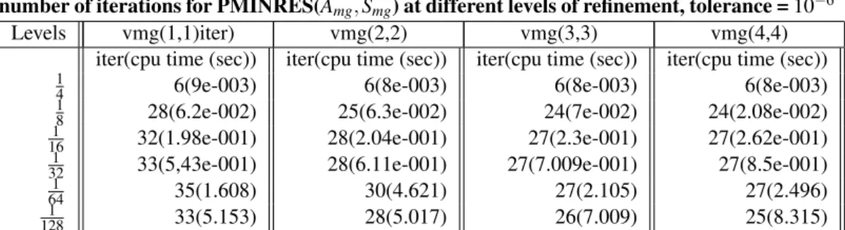
The Table (3) shows the effects of different multigrid v-cycle (1, 2, 3, 4) pre-and post-smoothing steps in the performance of the PMINRES method.
The results in Table (3) indicate that there is no significant difference in the performance of the PMINRES with multigrid preconditioner approximation of the preconditioner of A and Schur compliment S using pressure mass ma-trix Q. In the next table we present results of the PMINRES with multigrid v-cycle approxima-tion of the Laplacian combined with different approximations of the Schur compliment using the mass pressure matrix Q.
Table 1 Refinement levels and number of nodes(nl= number of velocity unknowns(×2) andml number of pressure unknowns)
refinement level(l) 1 2 3 4 5 6 7 8
mesh size(hl) 12 14 18 161 321 641 1281 2561 velocity nodes(nl) 9 25 81 289 1089 4425 16641 66049 pressure nodes(ml) 4 9 25 81 289 1089 4425 16641
Table 2 CPU time and number of iterations for PMINRES for different preconditioner
approximations at different levels of refinement, tolerance =10−6
Level Minres Pminres(diag(A),diag(Q)) iter(cpu time (sec)) iter(cpu time (sec)) 1
4 12(1.349) 12(4.4e-002)
1
8 59(1.6e-002) 33(1.9e-002)
1
16 231(1.57e-001) 86(1.00e-001) 1
32 529(8.11e-001) 182(5.78e-001) 1
64 1012(5.68) 386(4.621)
1
128 1845(4.11754e+001) 1008(5.0165e+001)
Table 3 CPU time and
number of iterations for PMINRES(Amg,Smg) at different levels of refinement, tolerance =10−6
Levels vmg(1,1)iter) vmg(2,2) vmg(3,3) vmg(4,4)
iter(cpu time (sec)) iter(cpu time (sec)) iter(cpu time (sec)) iter(cpu time (sec)) 1
4 6(9e-003) 6(8e-003) 6(8e-003) 6(8e-003)
1
8 28(6.2e-002) 25(6.3e-002) 24(7e-002) 24(2.08e-002)
1
16 32(1.98e-001) 28(2.04e-001) 27(2.3e-001) 27(2.62e-001) 1
32 33(5,43e-001) 28(6.11e-001) 27(7.009e-001) 27(8.5e-001) 1
64 35(1.608) 30(4.621) 27(2.105) 27(2.496)
1
128 33(5.153) 28(5.017) 26(7.009) 25(8.315)
Table 4 CPU time and number of iterations for PMINRES for different preconditioner
approximations at different levels of refinement, tolerance =10−6
Levels pminres(Amg,Smg) pminres(Amg,Spcg) pminres(Amg,Schebv) pminres(Amg,diag(Q)) iter(cpu time (sec)) iter(cpu time (sec)) iter(cpu time (sec)) iter(cpu time (sec)) 1
4 6(8e-003) 6(9.5e-002) 6(3.2e-002) 6(9e-003)
1
8 24(2,08e-001) 24(8.3e-002) 22(6.8-002) 21(5.6e-002)
1
16 27(2.62e-001) 29(2.81e-001) 25(2.41e-001) 40(3.24e-001) 1
32 27(8.5e-001) 29(2.9e-001) 27(8.08e-001) 44(3.4e-001) 1
64 27(2.496) 29(2.81) 27(8.08e-001) 44(1.136)
1
128 25(8.315) 29(9.252) 25(8.318) 44(1.29e+001)
Table 5 Changes in thek∇·ukΩ estimated velocity divergence error.ηthe global error
estimator from one level to the other
level 14 18 161 321 641 1281
k∇·ukΩ 2.230e-001 7.6e-002 2.016e-002 5.1e-003 1.28e-003 3.2e-004
η 2.6543 1.065e+000 2.773e-001 6.87e-002 1.71e-002 4.24e-003
iterative counts and the time are more attrac-tive as compared to the other preconditioner ap-proximations combinations like preconditioned conjugate gradient and diagonal preconditioner of the pressure matrix. The multigrid method proves to be a suitable approximation for the matrix A from the Laplacian. This agrees with the results in Peterset al.(2005) and the Cheby-shev iteration becomes a better approximation for the Schur compliment preconditioner using
the pressure mass matrix. The results show that the PMINRES is robust because the iterative counts do not change significantly as the matrix size increases.
as by the combination of the energy norm of the velocity error and theL2norm of the divergence error that is
η2
T :=k∇eT k2T +kRT k2T
Where eT is the velocity error estimate and
RT =k ∇·ukT and η:= (∑T∈Thη
2 T)
1
2 the
global error estimator. From the Table 5 we note that the velocity divergence is clearly converg-ing at a faster rate toO(h4), which means the estimated global errorηis increasingly domi-nated by the velocity error component ash→0
The changes in the solution errors are high-lighted in the table 5 below for the levels with mesh sizes14to 641.
The Fig. 1 below shows the sample snapshot of the grid output of residual reduction at the level with mesh size321 for MINRES and PMINRES. The Fig. 1 below the PMINRES residual error reduction is faster and is done in fewer iterations as compared to the MINRES. This is a reflec-tion that the precondireflec-tioners were very effective in making the solver perform very well.
The most interesting observation on the
fig-ures and table 5 is that from the two iterative schemes we get the same solution and a poste-riori error estimates. The above figure on the residual reduction clearly shows that the PMIN-RES is faster than the MINPMIN-RES. This shows that the accelerator is effective in improving the per-formance of the MINRES method. Hence pre-conditioning is an effective way of improving the performance of the iterative schemes. The use of the preconditioner in mandatory in mak-ing the iterative schemes effective and robust
0 100 200 300 400 500 600
10−6
10−5
10−4
10−3
10−2
10−1
100
101
iterations
log
10
(residual)
residual reduction
0 5 10 15 20 25 30
10−5
10−4
10−3
10−2
10−1
100
101
iterations
log
10
(residual)
residual reduction
Fig. 1. Residual reduction for MINRES(left) and PMINRES(right) of the Stokes equation at level 5.
−0.5 0 0.5 −0.5
0 0.5
−1 0
1
−1 0 1 9 9.5 10
x 10−5 Estimated error
9.2 9.3 9.4 9.5 9.6 9.7 x 10⁻⁵
9.2 9.3 9.4 9.5 9.6 9.7 x 10⁻⁵
−0.5 0 0.5 −0.5
0 0.5
−1 0
1
−1 0 1 9 9.5 10
x 10−5 Estimated error
9.2 9.3 9.4 9.5 9.6 9.7 x 10⁻⁵
9.2 9.3 9.4 9.5 9.6 9.7 x 10⁻⁵
Fig. 2. Estimated errorηin the computed solution at level 5 for the MINRES(left) and
5. CONCLUSION
The objective of the work consisted of the de-veloping efficient and robust iterative solvers for the two dimensional steady state Stokes equations discretized by mixed finite element method Q2−Q1 stable pair of rectangular el-ements. To this end, a MINRES method and its preconditioned counterpart denoted by PMIN-RES were used as solution schemes. In this pa-per we presented results for the MINRES and PMINRES that were considered through tradi-tional benchmark lid-driven cavity domain. For PMINRES we applied a combination of the pre-conditioners with the main diagonal approxi-mated by different iterative scheme. The pre-conditioner diagonal element Ab was approxi-mated by the multigrid v-cycle for all the tests since it is the best known solver for the Lapla-cian and different approximations were used for the Schur compliment. A comparative study was also made on the performance of the MIN-RES and PMINMIN-RES iterative schemes in terms of iterative counts and cpu time. We advocate the use of the multigrid preconditioner approx-imation for the Laplacian matrix A-block with the combination of the multigrid/Chebyshev semi iteration approximation for the Schur com-pliment to accelerate the performance of the MINRES iterative scheme. This entails that the multigrid solver is effective in accelerating the performance of the MINRES iterative scheme as justified by the numerical results. Hence it represents a robust and efficient solver of the Stokes problem. In most applications the MIN-RES (without preconditioning) is not an alter-native since it is expensive and requires direct inversion of a huge sparse matrix.
ACKNOWLEDGEMENTS
The authors wish to acknowledge the financial support from University of Venda.
REFERENCES
Benzi, M. and G. H. Golub and J. Liesen (2005). Numerical Solution of saddle point problems.Acta Numer. 14, 1–137. Braess, D. (2007).Finite Elements. London:
Cambridge University press.
Bramble, H. J. and J. E. Pasciak (1999). A preconditioning technique for indefinite systems resulting from mixed approxi-mations of elliptic problems. Mathemat-ics of Computation. 69, 667–689. Bramble, H. J., J. E. Pasciak and A. T.
Vassilev (1997). Analysis of the inexact Uzawa algorithm for saddle point
prob-lems. SIAM J. Numer. Anal. 34, 1072– 1092.
Brenner, C. S. and R. L Scott (2008). The Mathematical Theory of Finite Element Methods. New York: Springer.
Brezinski, C. (2005). Basics of Fluid Me-chanics and Introduction to Computa-tional Fluid Dynamics: Numerical Meth-ods and Algorithms. Boston: Springer. Cebeci, T., J. Shao, F. Kafyeke and E.
Lau-rendeau (2005). Computational Fluid Dynamics for Engineering. New York: Horizons Publishing.
Ciarlet, P. G. (1978). The Finite element methods for elliptic problems. Amster-dam: North- Holland Publishing Com-pany.
Donea, J. and A. Huerta (2003).Finite Ele-ment Methods for Flow Problems. West Sussex: John Wiley and Sons.
Elakkad, A., A. Elkhalfi and N. Guessous (2010). A mixed finite element method for Navier-Stokes equations. J. Appl. Math. and Informatics. 28 (5), 1331– 1345.
Elman, C. H. (2007). Algorithm 866. ifiss a matlab toolbox for modeling incom-pressible flow. ACM Transactions on Mathematical Software. 33 (2), article 14.
Elman, C. H. and H. G. Golub (1994). Inex-act and preconditioned Uzawa algorithm for saddle point problem. SIAM. J. Nu-mer. Anal. 31(6), 1645–1661.
Elman, C. H., D. Silvester, D. Kay and A. Wathen (1999). Efficient preconditioning of linearised Navier Stokes Equations. CS-TR 4073.
Elman, H. C., D. J. Silvester and A. Wathen (2005).Finite Elements and Fast Itera-tive Solvers: With Applications in Incom-pressible Fluid Dynamics. Oxford: Uni-versity Press.
Ferziger, J. H. and M. Peric (2002). Com-putational Methods for Fluid Dynamics. Berlin: Springer.
Girault, V. and P. Raviart (1986). A finite elements approximation of the Navier-Stokes equations. Berlin: Springer. Gockenbach, M. S. (2006). Understanding
Gunzburger, M. (1989). Finite Element Method for Viscous Incompressible Flows. New York: Academic Press. Hackbucsh, W. (1985). Multigrid methods
andapplications. New York: Springer. Herzog, R. and E. W. Sachs (2005).
Pre-conditioned conjugate gradient method for optimal control problems with con-trol and state constraints. SIAM. J. Ma-trix. Anal. Appl. 31, 2291–2317.
Larin, M. and A. Reusken (2008). A compar-ative study of efficient itercompar-ative solvers for generalised Stokes equations.Numer. Linear. Algebra Appl. 15, 13–34. Paige, C. G. and M. A. Saunders (1975).
So-lution of sparse indefinite systems of lin-ear equations. SIAM J. Numer.Anal. 12, 617–629.
Peters, J., V. Reichelt and A. Reusken (2005). Fast iterative solvers for the gen-eralised Stokes equations. SIAM J. Sci. Comput. 27, 1646–666.
Rees, T. and M. Stoll (2010). Block-triangular preconditioners for PDE-constrained optimization.Numer. Linear. Algebra. Appl to appear.
Rehman, U. M. and C. Vuik (2007). A com-parison of preconditioners for incom-pressible Navier- Stokes solvers. Int. J. Numer. Meth. Fluids. 57, 1731–1751. Reusken, A. and S. Gross (2011).
Numeri-cal methods for two-phase incompress-ible flows. Berlin: Springer.
Schorbel, J. and W. Zulehner (2007). Sym-metric indefinite precondotioners for saddle point problems with applications
to PDE-constrained optimisation prob-lems. SIAM. Math. J. Matrix. Anal. Appl. 29, 752–773.
Shaughnessy, E. and M. I. Katz and P. J. Schaffer (2005). Introduction to Fluid Mechanics. Berlin: Oxford University Press.
Stoll, M. and A. J. Wathen (2008). Combination preconditioning and the Bramble-Pasciak+ preconditioner. Acta Numer. 30, 582–608.
Tu, J., H. G. Yeoh and C. Liu (2008). Com-putational Fluid Dynamics: A Practical Approach. Oxford: Elsevier Inc.
Turek S. (1999).Solvers for incompressible flow problems. Berlin: Springer.
Vuik, C. (1996). Fast iterative solvers for discretised incompresible Navier Stokes equations. Int. J. Numer. Meth. Flu-ids. 22, 195–210.
Wathen, A. J. and T. Rees (2009). Cheby-shev semi-iteration in preconditioning for problems including the mass ma-trix.Electronic Transactions on Numer-ical Ananlysis. 34, 125–135.
Wesseling, P. (1999). An introduction to multigrid methods. New York: John Wi-ley and Sons Ltd, Chichester.
Zulehner, W. (2000). A class of smoothers for saddle point problems. Comput-ing. 65(3), 227–246.