HYBRID ONLINE MOBILE LASER SCANNER CALIBRATION THROUGH IMAGE ALIGNMENT BY MUTUAL INFORMATION

HYBRID ONLINE MOBILE LASER SCANNER CALIBRATION THROUGH IMAGE

ALIGNMENT BY MUTUAL INFORMATION

Mourad Miled, Bahman Soheilian, Emmanuel Habets, Bruno Vallet

IGN, Laboratoire MATIS 73 avenue de Paris 94165 Saint-Mand´e, FRANCE

bruno.vallet@ign.fr recherche.ign.fr/labos/matis/∼vallet

Commission IWG I/3

KEY WORDS:Calibration, Registration, Mobile Laser Scanning, Mobile Mapping

ABSTRACT:

This paper proposes an hybrid online calibration method for a laser scanner mounted on a mobile platform also equipped with an imaging system. The method relies on finding the calibration parameters that best align the acquired points cloud to the images. The quality of this intermodal alignment is measured by Mutual information between image luminance and points reflectance. The main advantage and motivation is ensuring pixel accurate alignment of images and point clouds acquired simultaneously, but it is also much more flexible than traditional laser calibration methods.

1. INTRODUCTION

1.1 CONTEXT

Mobile mapping systems are becoming more and more widespread because of their ability to capture extremely accurate data at large scale. Mobile mapping faces numerous challenges:

• Volume of data acquired calling for very efficient processing to scale up

• Complexity of the captured 3D scenes (occlusions, radiom-etry, mobile objects,...)

• Localisation accuracy: GPS outage are frequent in city cores and may lead to large geolocalization errors.

Whereas mobile mapping systems have been traditionally divided between laser and image based platforms, hybrid systems (with both image and laser sensors) are getting more and more popu-lar.For such systems, the laser and image sensors are calibrated independently using standard calibration procedures. In our ex-perience, such independent calibration methods may lead to reg-istration errors of a few pixels between the image and laser data (cf figure 2). We believe that reducing this error below a pixel may unlock new applications for hybrid systems such as:

• Joint image/laser scene interpretation

• Joint image/laser 3D surface reconstruction and texturing

(Vallet et al., 2015) also advocates that precise image/laser align-ment is required for mobile objects delineation in images. More-over, the method that we propose is online, meaning that it does not require a special acquisition in a specially equipped site to perform the calibration, and that it can be used to assess the sta-bility of image and laser calibrations in time.

Figure 2: Image/laser superposition on a zoom of Figure 1 show-ing a calibration error of a few pixels

1.2 RELATED WORKS

A calibration method is characterized by:

• The features: what is matched between the two sources ? It can be known targets, feature points (Chen and Tian, 2009), regions (Liang et al., 1997), edges or primitives, in which case the method is calledsparse, or the points/pixels com-posing the data, in which case the method is calleddense.

• Similarity measure: how good are the matches ?

• Deformation model: how is a source deformed to align to the other ? (rigid, non-rigid, affine...)

• Optimisation: which deformation ensures the best similarity ? Note that whereas optimization often aims at minimizing an energy, here we maximize similarity.

Sparse methods use high level features which are more discrim-inative and lead to a simpler optimization. Plenty of detectors ensure invariance to orientation, scaling, perspective, lighting,... However it might be difficult to find features invariant across modalities and accurate enough, and different features might be detected in the sources leading to error prone feature matching. Conversely, dense methods do not rely on feature detection but only on the similarity measure, which is more simple and yields alignment information over the whole data. However the opti-mization is more intensive and the similarity measure can be less discriminative than features.

For sparse method, the similarity measure is dependent on the features: based on SIFT descriptors, region shapes, geometric distance between primitives... For dense methods, the most sim-ple measure is the (point to point or point to triangle) squared dis-tance for point clouds, and Zero mean Normalized Cross Corre-lation (ZNCC) for images. For multimodal registration, the Mu-tual Information (MI) (Mastin et al., 2009) is often preferred. MI measures statistical co-occurrence between values of correspond-ing points/pixels by computcorrespond-ing their joint histogram. A flat his-togram indicates no correlation, whereas strong maxima indicate high correlation.

Finally, the optimization problem has the form:

max

t∈Tf(I1, t(I2)) (1)

• I1etI2are the data sources

• t: transformation to apply toI2to align it withI1

• T: set of possible transformations

• f: similarity measure

For a rigid transform,Tis parametrized by the 3 components of a translation (the lever-arm) and the 3 bore-sight angles. For a mobile laser scan, this transformation is expressed in a mobile frame so the resulting transform is not a rigid transform, even if it has the same parameters. To optimize these parameters, three classes of methods may be used:

Closed form For least squares similarity measure and simple transform space, the optimal transform can be expressed directly in closed form.

Gradient-based If the gradient is easy to compute, it can guide the optimization by following the steepest ascent line. Such method converge rapidly to a precise optimum but for non convex ener-gies, this optimum can be local without guarantee that the global optimum is reached. The various methods (gradient descent, New-ton’s method, Levenberg-Marquardt, conjugate gradient) mainly differ on the exact choice of the direction and of the step length. If uncertainties on the inputs are known, then the Gauss-Helmert method can be used (McGlone et al., 2004).

Gradient-free If the gradient is hard to compute or if the en-ergy has many local optimas, a gradient free method can be pre-ferred. Gradient free methods will evaluate the similarity on samples of T with various heuristics to choose the next sam-ples. Monte Carlo methods sample the space with a random distribution that becomes concentrated near local optimas as a temperature parameter decreases. The bats algorithm evolves a population of samples inspired by the behaviour of herds. Ge-netic algorithms randomly combine the best previous solutions into new ones. The Nelder-Mead (or simplex) algorithm (Deng et al., 2008) evolves a simplex toward the optimum according to the similarity measure on its vertices. The conjugate Powell al-gorithm (Maes et al., 1997) iterates optimization over individual parameters.

1.3 DATA PRESENTATION

Figure 3: A set of images acquired for one pose (panoramic + 2 stereo pairs)

The data used in this study was acquired by the mobile mapping system (MMS) described in (own citation). It is equipped with 14 full HD (1920×1080px) cameras acquiring 12 bits RGB images (8 images panoramic + 2 stereo pairs) as shown in figure 3.

Figure 4: A view of the Mobile Laser Scan (MLS) used in this study, coloured with reflectance.

The laser sensor is a RIEGL LMS-Q120i that was mounted transver-sally in order to scan a plane orthogonal to the trajectory. It ro-tates at 100 Hz and emits 3000 pulses per rotation, which corre-sponds to an angular resolution around0.12◦

. Each pulse can result in 0 to 8 echoes producing an average of 250 thousand points per second. In addition to the (x, y, z)coordinates (in sensor space), the sensor records multiple information for each pulse (direction, time of emission) and echo (amplitude, range). The amplitude being dependant on the range, it is corrected into a relative reflectance. This is the ratio of the received power to the power that would be received from a white diffuse target at the same distance expressed in dB. The reflectance represents a range independent property of the target.

The MMS is also mounted with an Applanix POS-LV220 geo-referencing system combining D-GPS, an inertial unit and an odometer. The laser sensor is initially calibrated by topometry in order to recover the transformation between the sensor and Ap-planix coordinate systems which allows to transform the(x, y, z)

coordinates from sensor to a geographic coordinate system. The result, with a colormap on reflectance, is displayed in Figure 4.

The point cloud is acquired continuously in time, such that when projecting a point cloud to an image, some projected points may have been acquired a few moments before or after the moment the image was acquired.

2. METHODOLOGY

2.1 FRAMES

In this work, we callTαβthe rigid transforms defined by a rota-tionRαβand a translationTαβ that transform point coordinates

xαin frameαto coordinatesxαin frameβ:

xβ=Tαβxα=Rαβxα+Tαβ (2)

These transforms link the 4 following frames:

• TheWorld frameWattached to the scene

• TheVehicle frameV attached to the vehicle and given by its geopositionning system. It depends on time as the vehicle moves, and is defined byTV W(t)

• TheLaser frameLattached to the laser that produces point coordinatesxLi in this frame (iis the point index). The ob-ject of this work is estimatingTa

LV, through its parameters

a= (tx, ty, tz, θx, θy, θz)whereTLVa is the translation of vector(tx, ty, tz)and

Ra LV =





czcy czsysx−szcx czsycx+szsx

szcy szsysx+czcx szsycx−czsx −_{sy cysx cycx}



 (3)

c•= cos(θ•) s•= sin(θ•)

• TheCamera frame defined byTCV that we assume known (already well calibrated). Assuming that the image has been resampled to compensate for lens distortion, the image pixel coordinates are defined fromCamera coordinates by a sim-ple pinhole model:

pCI(xC) =

xC

zC

yC

zC

(4)

Using these notations, and knowing the exact timestiat which each 3D pointxLi is acquired, andtIat which imageIwas ac-quired, we can define the projection of a laser pointxL_inI:

pa_(xL_{) =}

pCI◦TV C◦TW V(tI)◦TV W(ti)◦TaLV(x L

) (5)

In this framework, re-estimatingTLV does not lead to a rigid transform of the pointcloud asTV W(ti)depends on the acqui-sition time of each point which is illustrated on Figure 5. The estimation of TLV will be performed by maximizing over the transformation parameters r a similarity measure between the reflectance measured on 3D points and the corresponding lumi-nance on the pixels on which they project.

2.2 MUTUAL INFORMATION

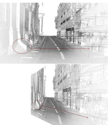
Figure 5: Non rigid transform of a mobile laser scan induced by a rigid transform on the laser frame of45◦

around the vertical yaw axis. Top: Mobile laser scan with correct calibration, Bot-tom: Mobile laser scan with calibration rotated. Scanlines are not orthogonal to the trajectory any more

one with smallest depth in case more than one point projects in the same pixel, and we callPi i = 1..nthese points. For the MI to be comparable between iterations, this set will not be re-evaluated. The features correlated will be the laser reflectanceRi of pointiand the image luminanceL(pa_(xL

i)) =Lai estimated from the RGB components for the image (cf figure 1).

Computing MI relies on computing a joint (2D) histogram of these features over such correspondences:

M I(a) =

nLbin X

L=1 nRbin X

R=1

plr(L, R,a)log

_p

lr(L, R,a)

pl(L, r)pr(R)

(6)

wherenL

bin and nRbin are the respective number of bins of the

Luminance andReflectance histograms. For simplicity, we as-sume thatLa

i andRiare normalized to lie in[0, nLbin+ 1]and

[0, nR

bin+ 1]. With this convention:

pl(L,a) =

1

n

n

X

i=1

φ(La

i−L) pr(R) =

1

n

n

X

i=1

φ(Ri−R) (7)

plr(L, R,a) =

1

n

n

X

i=1

φ(La

i −L)φ(Ri−R) (8)

φ(t) = 





t+ 1 if t∈[−1; 0]

−t+ 1 if t∈[0; 1]

0 else

(9)

allows to associate a feature value to the two closest bins.

2.3 LEVENBERG MARQUARDT OPTIMIZATION

We have explained how to compute the MI for a given trans-forma. The online calibration proposed in this paper relies on

finding the optimal transforma∗

that maximizes the MI. As we can assume a good initializationa0 (calibration by topometry for instance), we chose a gradient descent algorithm: Levenberg-Marquardt (LM). LM optimizes the MI iteratively by:

at+1=at−(H+µ.diag(H)) −1

GT (10)

whereGis the gradient andHthe Hessian of the MI andµthe so-calleddampingfactor. The gradient computation goes following (Dame and Marchand, 2011) and (Dowson and Bowden, 2006):

G=∇_aM I(a) = X

L,R

∇_aplr(L, R,a)

1 +log

plr(L, R,a)

pl(L, r)

(11)

∇aplr(L, R,a) =

1

n

X

i

∇aφ(L a

i −L)φ(Ri−R) (12) ∇aφ(L

a

i −L) =∇aL a iφ

′

(La i −L)

=∇_apa_∇ pL

a iφ

′

(La

i −L) (13) where:

φ′

(t) = 





1 if t∈[−1; 0]

−₁ if t∈_{[0; 1]}

0 else

(14)

and ∇_pLa

i is simply the image luminance gradient (estimated atpa_(xL

i)by bilinear interpolation). Calling∇α the derivative along coordinates in frameαand applying it to (2), we get:

∇_αxβ=∇_αTαβxα=Rαβ (15) so from (5) we get:

∇ap a

=∇CpCIRV CRW V(tI)RV W(ti)∇aT a LVx

L (16)

where:

∇CpCI(xC) =

" 1 zC 0

−xC

z_C2

0 1

zC −

yC

z2 C

#

(17)

and following (Chaumette and Hutchinson, 2006):

∇aT a LVx L =  

−1 0 0 0 −zL _yL

0 −1 0 zL _{0 −x}L

0 0 −1 −yL _xL ₀



 (18)

Finally the Hessian is simplified as:

H=∇T_aG=−X L,R ₁ plr − 1 pl

∇T_aplr∇aplr+

plr

pl ∇2_aplr

(19) As advised in (Dowson and Bowden, 2006), we will neglect the second derivative∇2

aplras it is approximately zero near the min-imum, so its use only improves the speed of optimisation slightly at great computational expense. Consequently, the final Hessian computation only requirespl,plrand its partial derivatives. After each iteration, we get the new transformation parameters. Theµ

control parameter defines how far we go along the gradient direc-tion. The largerµ, the smaller are the corrections.µis initialized at210_{= 1024}

and adjusted at each iteration: if the MI increases,

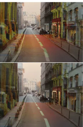
Figure 6: Place de la Bastille - Before (top) and after (bottom) hybrid calibration

3. RESULTS

3.1 EXPERIMENTS

Results the image/laser calibration method described above on a first example (Place de la Bastille in Paris) are presented in Figure 6. The quality of the result is evaluated qualitatively on some close-ups shown on Figure 7.

The MI similarity measure decreases from 25.37% for the initial calibration to 29.12%. Figure 8 gives the evolution of the MI through LM iterations.

A second example (Saint Sulpice church in Paris) is presented in figure 9) with close ups in Figure 10. On that example, we vol-untarily perturbated the initial calibration to assess the robustness of the method, which explains the larger error.

Because of this higher initial error, the MI increases more sig-nificantly from 14.57% to 21.02%. The evolution of MI through iterations is displayed in Figure 11.

3.2 DISCUSSION

3.2.1 INFLUENCE OF THE NUMBER OF BINS The im-age grey level is in [0, 255] and laser reflectance in [-20dB, 0dB]. These intervals are split in bins to create the histogram. Larger bins reduce computation time and ensure more robustness to noise. The best results were obtained for 32 bins for image gray level and 16 bins for laser reflectance. However, a low number of bins might lead to low precision, so after a first convergence, a few more iterations can be performed with an increased number of bins.

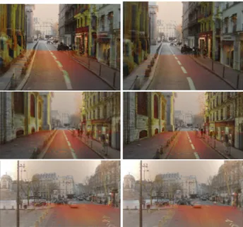
Figure 7: Place de la Bastille - Close up on the red (top), blue (middle) and green (bottom) parts before (left) and after (right) hybrid calibration

Figure 9: Saint Sulpice area before (top) and after (bottom) hy-brid calibration

Figure 10: Saint Sulpice: close up on road marks (top) and on the left sidewalk (bottom) before (left) and after (right) hybrid calibration

Figure 11: Convergence of LM for the Saint Sulpice dataset.

Figure 12: Calibration result on a road mark

3.2.2 ACCURACY Our initial objective of pixel accuracy is only possible for points acquired close enough (in time) to the im-age as the georeferencing drifts in time. For points further away (in time) we observed an error up to 3 pixels after calibration (cf Figure 12). The intrinsic calibration of the image might also lead to errors of around one pixel.

3.2.3 ROBUSTNESS The MI similarity measure is quite ro-bust to multimodality and illumination changes. This is illus-trated in complex urban environments: narrow streets (Figure 9), large squares (Figure 6) or crossings (Figure 13). The calibration always reaches the correct optimum even in the Sain Sulpice ex-ample with perturbated input. Robustness to moving objects is also demonstrated on Figure 13: a bus has moved between the in-stant it was acquired by the image and the laser. Despite its large size, the resulting calibration is still accurate.

3.2.4 STABILITY To measure the stability of our hybrid cal-ibration, we applied it independently to 3 image/laser couples from the same acquisition but separated by a few minutes each (Figure 14). Convergence was achieved in the 3 cases and the resulting parameters vary of a few centimetres for the translation and below0.001◦

for rotation.

Figure 14: Saint Sulpice results on three extracts before (left) and after (right) hybrid calibration

The relatively low stability for translation is in contradiction with the pixel accuracy that we observe in the results. The reason is probably that the translation part of the calibration compensates for the georeferencing drift that varies in time.

4. CONCLUSION

Mutual Information (MI) is a powerful, precise and dense mea-sure that is well adapted to aligning image and laser data. It is robust to illumination variations, multimodality, occlusions and mobile objects because its exploits all the information contained in the image and mobile laser scan.

Its computation time (3 to 7 minutes depending mostly on the number of 3D points projected in the image) is completely ac-ceptable for the typical use scenarii:

• Laser calibration on an area with good GPS visibility in or-der to limit the impact of georeferencing errors.

• Calibration on a few extracts of each acquisition performed by a mobile platform in order to assess the stability of the calibration through time.

In the future, we aim at improving the method in several manners:

• Handling multiple images instead of a single one

• Authorizing deformations of the laser scan to compensate for the georeferencing drift, or using image/laser attachment in a more global registration procedure.

• Selecting the 3D points to project with a fine point visibility computation.

REFERENCES

Chaumette, F. and Hutchinson, S., 2006. Visual servo control. i. basic approaches. Robotics & Automation Magazine, IEEE 13(4), pp. 82–90.

Chen, J. and Tian, J., 2009. Real-time multi-modal rigid regis-tration based on a novel symmetric-sift descriptor. Progress in Natural Science 19(5), pp. 643–651.

Dame, A. and Marchand, E., 2011. Mutual information-based visual servoing. Robotics, IEEE Transactions on 27(5), pp. 958– 969.

Deng, F., Hu, M. and Guan, H., 2008. Automatic registration be-tween lidar and digital images. The International Archives of the Photogrammetry, Remote Sensing and Spatial Information Sci-ences pp. 487–490.

Dowson, N. D. H. and Bowden, R., 2006. A unifying framework for mutual information methods for use in non-linear optimisa-tion. In: Proc. Eur. Conf. Comput. Vis., vol. 1, pp. 365–378.

Le Scouarnec, R., Touz´e, T., Lacambre, J.-B. and Seube, N., 2013. A position free calibration method for mobile laser scan-ning applications. In: ISPRS Annals of the Photogramme-try, Remote Sensing and Spatial Information Sciences, ISPRS Workshop Laser Scanning 2013, 11-13 November 2013, Antalya, Turkey, Vol. II-5/W2.

Liang, Z.-P., Pan, H., Magin, R., Ahuja, N. and Huang, T., 1997. Automated registration of multimodality images by maximiza-tion of a region similarity measure. In: Image Processing, 1997. Proceedings., International Conference on, Vol. 3, pp. 272–275 vol.3.

Maes, F., Collignon, A., Vandermeulen, D., Marchal, G. and Suetens, P., 1997. Multimodality image registration by maxi-mization of mutual information. Medical Imaging, IEEE Trans-actions on 16(2), pp. 187–198.

Mastin, A., Kepner, J. and Fisher, J., 2009. Automatic registration of lidar and optical images of urban scenes. In: Computer Vision and Pattern Recognition, 2009. CVPR 2009. IEEE Conference on, IEEE, pp. 2639–2646.

McGlone, J. C., Mikhail, E. M. and Bethel, J. S., 2004. Manual of Photogrammetry. 5th edition edn, American Society of Pho-togrammetry and Remote Sensing.

Nouira, H., Deschaud, J. E. and Goulette, F., 2015. Target-free extrinsic calibration of a mobile multi-beam lidar system. In: IS-PRS Annals of the Photogrammetry, Remote Sensing and Spatial Information Sciences, ISPRS Geospatial Week, 28/09-3/10 2015, La Grande Motte, France, Vol. II-3/W5, pp. 97–104.

Rieger, P., Studnicka, N., Pfennigbauer, M. and Zach, G., 2010. Boresight alignment method for mobile laser scanning systems. Journal of Applied Geodesy 4(1), pp. 13–21.

Skaloud, J. and Lichti, D., 2006. Rigorous approach to bore-sight self-calibration in airborne laser scanning. ISPRS Journal of Photogrammetry and Remote Sensing 61(1), pp. 47 – 59.

Skaloud, J. and Schaer, P., 2007. Towards automated lidar bore-sight self-calibration. In: A. Vettore and N. El-Sheimy (eds), The 5th International Symposium on Mobile Mapping Technol-ogy (MMT ’07), May 29-31, 2007, Padua, Italy, Vol. XXXVI-5/C55, ISPRS, p. 6.