0103 - 5053 $6.00+0.00
A
r
ti
c
le
*e-mail: [email protected]
Validation of Multivariate Calibration Models in the Determination of Sugar Cane Quality
Parameters by Near Infrared Spectroscopy
Patrícia Valderrama, Jez W. B. Braga and Ronei J. Poppi*
Instituto de Química, Universidade Estadual de Campinas, CP 6154, 13084-862 Campinas-SP, Brazil
Os teores de sólidos solúveis (BRIX), açúcares polarizáveis (POL) e açúcares redutores (RS) em caldo de cana foram determinados utilizando espectroscopia na região do infravermelho próximo (NIR) e calibração multivariada, a qual foi validada pelo cálculo das figuras de mérito. Devido à heterogeneidade das amostras, foi necessário, como primeira etapa do trabalho, a otimização dos conjutos de calibração e validação através da eliminação das amostras anômalas (outliers). As figuras de mérito como: sensibilidade, sensibilidade analítica, seletividade, limites de confiança, precisão (média, repetibilidade), exatidão e razão sinal-ruído foram calculadas. Resultados viáveis foram obtidos para BRIX e POL apresentando resultados de RMSEP de 0,28 e 0,42% de caldo, respectivamente. Os coeficientes de correlação para ambos os parâmetros foram de 0,99. Estes resultados indicam que os modelos desenvolvidos para BRIX e POL podem ser seguramente utilizados como uma alternativa em relação ao método padrão utilizado na indústria alcooleira.
The determination of soluble solids (BRIX), polarizable sugars (POL) and reducing sugars (RS) sugar cane juice by using near infrared spectroscopy (NIR) and multivariate calibration was developed and validated by calculation of figures of merit. Due to the heterogeneity of the samples, first it was necessary to optimize the calibration set by outlier elimination. The figures of merit such as: sensitivity, analytical sensitivity, selectivity, confidence limit, precision (mean, repeatability), accuracy and signal-to-noise ratio were calculated. Feasible results were obtained for BRIX and POL with RMSEP values of 0.28 and 0.42% of juice and precision of 0.02 and 0.08% of juice, respectively. For both BRIX and POL goodness of fit showed correlation coefficients of 0.99. These results indicate that the models developed for BRIX and POL can be used as an alternative to standard procedures in the sugar cane industry.
Keywords: sugar cane, multivariate calibration, net analyte signal, figures of merit
Introduction
Nowadays, the industrial production of alcohol (ethanol) in Brazil has become a strategic area due its applicability as an alternative fuel, since sugar cane is the
basic raw material for its manufacture.1The sugars of cane
are basically represented by sucrose, glucose and fructose.
Sucrose (C12H22O11) is a disaccharide which constitutes
the principal parameter of quality of sugar cane and under acid conditions, or action of enzymes, is unfolded to its monosaccharide molecules, which causes a decrease in alcohol production. Glucose and fructose are also called reducing sugars, because they have the property of
reducing copper from the Cu2+ state to Cu1+.2,3In the
calculation of sugar cane costs by industry, the main
parameter used is the cane quality, estimated according to its concentration in recoverable total sugar (RTS), which is function of polarizable sugar (POL), soluble solids
(BRIX) and reducing sugars (RS).3,4The parameters
mentioned above are estimated by measurement with saccharimeters, densimeters and oxidation-reduction titrations, respectively, as standard methodologies, that are regulated by norms of evaluation of the quality of sugar cane.
BRIX can be defined as the percentage in weight, or in volume, of soluble solids expressed as sucrose. In sugar cane juice it is a quantitative measurement of the total solids (including sugars), not giving any qualitative information about which sugars are present in the final
product.3 POL is a measurement of the amount of sucrose
in the mixture of sugars, because in it, only sucrose diverts
oxidation-reduction titration. However, for sugar cane grower payment, RS is not determined via analysis, but is just estimated by an equation that takes in consideration
the BRIX and POL parameters.3
Alternative methods of analysis for sugar cane grower payment, such as mid infrared spectroscopy and fluorescence, have been investigated and tested, with the aim to increase the reliability, uniformity of the method
and the accuracy of the measurements.5,7Near infrared
spectroscopy (NIR) has been recently investigated as an alternative methodology, due its special characteristics such as non-destructivity, quickness and no production of
offensive wastes.8-13 Nowadays, some distilleries in Brazil
have began the implementation of this analytical methodology. In this case, the application of NIR should be validated using an independent data set and by calculation of figures of merit to certify its ability to predict the properties of interest. However, based on the
reference norm3 actually employed, figures of merit are
not calculated.
The aims of this work were built and validate multivariate calibration models for determination of BRIX, POL and RS using the near infrared spectra of cane juice. For this purpose, figures of merit such as: sensitivity, analytical sensitivity, selectivity, confidence limit, precision (mean, repeatability), accuracy and signal-to-noise ratio were calculated, and the model results were compared with reference values obtained by the standard methods to confirm the applicability of the proposed methodology.
Experimental
The experimental measurements of this work were accomplished at alcohol plant Cocamar - Cooperativa Agroindustrial, located at São Tomé city in the State of Paraná - Brazil.
Ripe cane sugar arrives in the industry transported by trucks and were sampled by horizontal probe. Samples were cut and carried to the laboratory. In the laboratory,
the samples were pressed to 250 kgf cm-2 in an hydraulic
press for a period of 1 minute, resulting in the cane juice for subsequent analysis. Finally, before the spectra acquisition, the samples were filtered in cotton to eliminate suspended particles.
Spectra were collected at a NIRSystems spectrometer, model 5000 monochromator, equipped with a tungsten filament source, quartz cuvette of 1 mm of optical path and a PbS detector. Acquisition of the spectra was accomplished in the range of 1100 - 2500 nm by using the ISIScan software.
A total of 1381 samples of sugar cane juice were used in this work. Each sample was submitted to conventional analysis and the results were used as reference values for model development.
The BRIX values were obtained directly, using a digital
densimeter with a precision of 0.01 oBRIX. The POL
measurements were obtained in a digital saccharimeter with precision of 0.01. The samples of cane juice were initially
cleared with lead sub-acetate (Pb(CH3COO)2.Pb(OH)2) and
filtered before the measurements. The degree of polarization of the sample, expressed as % of juice, was calculated based on the saccharimeter reading (SR) and equation 1.
POL = SR (0.2605 – 0.0009882 BRIX) (1)
In RS determination, the standard methodology used was proposed by Eynon & Lane, which consists in the oxidation-reduction titration of the Fehling Liqueur by the filtered cane juice. RS (also expressed as % of juice) present in each sample was obtained by equation 2, taking into consideration the standard volume spent in the titration of the Felhling Liqueur solution by a solution of
1% of inverted sugar and the BRIX measurement.3
(2)
where VS is the volume of cane juice spent in the titration and Vs is the standard volume of the inverted sugar.
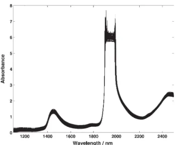
Figure 1 shows the spectra of all 1381 samples. These samples, for calculations purposes, were split in 1003 calibration samples and 378 validation ones, by using the
Kennard-Stone algorithm.14The intense band in the region
around 1900 nm was eliminated due the high water
absorption15 and mean centering was used for data
pre-processing. Calibrations models were developed using the PLS-Toolbox version 3.5 from Eigen_Vector Technology for Matlab 6.5, based on PLS1 method. The validation was accomplished by the calculation of figures of merit using Matlab routines developed in our laboratory.
Theory
The data matrix Xis formed by the NIR spectra of the
sugar cane juice and the vector y contains the reference
For the calculation of the NAS, the matrix X is rebuilt
based on A latent variables calculated by PLS, yielding
the matrix X^A. Subsequently, the matrix free from the
contribution of the analyte of interest k (X^
A,-k) is calculated
as:16
(3)
where^yA,k is the concentration vector ykprojected down
onto the A-dimensional space calculated by PLS and the ‘+’ superscript is the Moore-Penrose pseudoinverse. The NAS vector for the ‘i’ calibration or validation sample^ nxA,ak,si can be written as:
(4)
where I is the identity matrix of appropriate size and
x ^n
A,ak,si is the NAS vector. It is important to note that ^ nxA,ak,si
contains only the information of analyte k (BRIX, POL or RS), thus it is possible to replace it by its Euclidean norm, generating a scalar nas:
(5)
Since the experimental responses of analyte k can be expressed as a scalar value, an univariate inverse calibration model can be built by the least squares method as:
(6)
where nâscal.k and ycal,k are the NAS and the reference values
for the calibration samples and ^bnas,k is the regression coefficient
of the pseudo univariate model. If the data matrix was mean-centered, before of the determination of b^nas,k, the nâsi,k needs to be changed to avoid a signal error that is inserted by implementation of the Euclidean norm. This correction can
be performed by multiplication of the nâsi,k by the signal of
(yi – y–cal), where y–calis the respective analyte concentration
average of the calibration samples.17 The pseudo-univariate
model represents faithful the multivariate model in a simple form that can be presented as an usual analytical curve.
Analytical figures of merit
Accuracy reports the closeness of agreement between
the reference value and the value found by the calibration model. In Chemometrics, this is generally expressed as the root mean square error of the prediction samples (RMSEP), that is an approximation of the standard error
of the prediction samples, obtained as:18
(7)
where n is the number of prediction samples. The accuracy expressed by equation 7 assumes that the error in the reference values is neglected. In applications where this assumption can not be made this error should be taking count, as is discussed by Faber and
Kowalski.19
Precision represents the degree of scatter between a series
of measurements for the same sample under prescribed conditions. It is usually expressed as a standard deviation, or
relative standard deviation, of a series of measurements.20
(8)
where n is the number of samples and m the number of
replicates. In agreement with ASTM20 it should be determined
as the mean of the standard deviation of a minimum of six measurements on a minimum of three samples.
Signal-to-Noise Ratio in the univariate case this
parameter represents how much the signal of the analyte k is larger than the instrumental noise. In the present case,
this is calculated as:21
(9)
where Gx is an estimate for the instrumental noise,
calculated as the standard deviation of 15 blank samples.
Sensitivity this parameter informs what fraction of
analytical signal that is due to the increase of the concentration of a particular analyte at unitary concentration. In inverse
multivariate calibration models, it is defined as:21, 23
(10)
where the vector of sensitivities Sn
k
as must be the same
for all calibration samples,X^n
A,aks is the vector for the net
analyte signal for the k analyte and yi is the reference
value of the sample i. The sensitivity can be estimated as:
(11)
Analytical Sensitivity defined as the ratio between the
sensitivity and the instrumental noise:
(12)
The inverse of this parameter (γ-1) reports the minimum
concentration difference between two samples that can
be determined by the model.24
Selectivity in univariate calibration, selectivity is
defined as the extent to which the method can be used to determine particular analytes in mixtures or matrices without interferences from other components with similar
behavior.24 Otherwise, in multivariate calibration with the
use of NAS, it is calculated as a ratio of the scalar nasi
and the Euclidean norm of the original vector of the
instrumental responses xk,un:21
(13)
SÊL indicates the portion of the instrumental signal that is used for the multivariate calibration model.
Confidence Intervalsdefined as the range within which
it is possible to assume, with a given degree of confidence (it, a certain probability), that the true value of the concentration of the analyte of interest is included. It can be determined by a t-test and an approximate estimate for the variance of the prediction error (V(PE)). The V(PE) can be determined by the Errors in Variables (EIV)
theory,25 that under simplifications reduces to the equation
adopted in ASTM E1655-00,20 expressed as:
(14)
where MSEC is the mean squared error of calibration and
hunis a leverage for the prediction sample, defined as:18, 20
(15)
where TA is the score matrix of the calibration samples
andtun,A the score of an unknown sample. The number of
degrees of freedom used in the calculation of MSEC is determined by the approach of pseudo degrees of freedom
proposed by Van Der Voet.26
After V(PE) calculation of confidence intervals (f) can be obtained by:
(16)
where t is the statistical parameter of the t-Student
distribution.
Bias according to the IUPAC definition,23 bias is the
difference between the population mean and the true value. Systematic errors are all error components that are not random. Then, it is possible to equate systematic errors with the fixed bias of the chemical measurement process. The occurrence of systematic errors was investigated by
a t-test described in the ASTM E1655-00.20 First, an
average bias is calculated for the validation set:
(17)
where lv is the number of samples in the validation set. Then the standard deviation of validation (SDV) is obtained by:
(18)
Finally, the t value is given by:
(19)
If the t calculated is greater than the critical t value at the 95% confidence level, there is an evidence that the bias included in the multivariate model is significant.
Goodness of fit the evaluation of this parameter is
usually accomplished by a curve fitting of the prediction values versus the reference ones, calculation of the correlation coefficient, y-intercept and the slop of the
regression line.18 Another way to do this evaluation is to
use the net analyte signal calibration line, obtained by a
Linearity the evaluation of this figure of merit is
problematic in multivariate calibration using PLS, because the variables are previously decomposed by principal component analysis. The plot of residuals and scores versus the reference values is a qualitative estimate of the linearity of the model, where they must present random and linear behaviours, respectively. However, the score plot only can be used when the PLS model requires a few
latent variables to describe the data set.18
Limit of Detection (LOD) following the IUPAC
recommendations, the LOD can be defined as the minimum detectable value of net signal (or concentration)
for which the probabilities of false negatives (β) and false
positives (α) are 0.05.23 The LOD can be calculated
analogously as for univariate calibration:28-30
(20)
Limit of Quantification (LOQ) the ability of
quantification is generally expressed in terms of the signal or analyte concentration value that will produce estimates
having a specified relative standard deviation.23 Following
the same assumptions described above, the LOQ in
multivariate calibration has been calculated by:28
(21)
Results and Discussion
The calibration set was optimized by outlier
elimination, based on data with extreme leverage18 in
calibration, unmodelled residuals in spectral data20 and
unmodelled residuals in concentration (property of
interest).18 The outliers in validation set were determinated
by estimation of the extreme leverage and unmodelled residuals in spectral data. This procedures resulted in 897, 924 and 857 calibration samples and 362, 358 and 368 validation samples for BRIX, POL and RS, respectively. The optimum model dimension was determined by the minimum RMSECV (Root Mean Squares Error of Cross Validation) for the calibration samples, obtained by contiguos block cross validation of 10 samples. Four, six and four PLS factors for BRIX, POL and RS, respectively, were necessary to retain a significant variance in the data and to avoid a significant bias in the model. The presence of relevant bias was tested with the
prediction results for the validation samples by the t-test
suggested by ASTM E1655-00.20 The results showed that
the bias included in the model was not significant, since
the t values obtained 2.07, 1.37 and 2.17 for BRIX, POL and RS, respectively, were lower that the critical value of 2.576 with 99% of confidence.
Results for the figures of merit are presented in the Table 1. Accuracy values represented by RMSEC (Root Mean Square Error of Calibration) and RMSEP (Root Mean Square Error of Prediction) showed that the estimated values of all multivariate models presented good agreement with reference methods.
Precision, at level of repeatability, was assessed by analysis of three samples with six replicates each, in measurements made in the same day. The results for BRIX and POL showed that the multivariate models were better than the regulated norms of evaluation of the quality of the cane sugar that is 0.3% for BRIX and 0.6% for POL. For RS, feasible results were also observed, but there is no regulated norm for precision of this parameter, since in industry it is not determined experimentally but just estimated by an equation that takes in consideration the
BRIX and POL parameters.2 However, the value of RS is
important for grower payment in the industry.
For sensitivity and analytical sensitivity good results were observed for the three parameters studied, taking into account the analytical range of the models. Analytical sensitivity is simpler and more informative for comparison and to judge the sensitivity of an analytical method. It is possible to establish a minimum concentration difference which, in the absence of errors in the property of interest, is discernible by the analytical method in the range where it was applied. Based on this result, for BRIX it is possible to distinguish between samples with value differences of
around 0.22×10⁻² % / juice.
Results for signal-noise ratio showed in Table 1 are the maximum values observed for each parameter. These values, apparently low, did not present a direct relation with the prediction errors. A feasible explanation for these
results is that the estimates of the instrumental noise (Gx)
do not represent the whole data set. This result suggests that the estimated LD and LQ presented in Table 1 might be optimistic values.
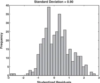
The error distribution for BRIX and POL parameters presented a random behavior, while for the RS parameter it a tendency (bias) was observed that reinforces the suspicion of non-linearity in the data set. Figures 5, 6 and 7 show the histograms for the student residuals for BRIX, POL and RS. These distributions resemble a gaussian behavior, but by using
a Jarque-Bera test,31 only for BRIX the student residuals are
normally distributed while for POL and RS significant differences from normality were observed. The CL values, estimated at 95% of probability by equation 16, demonstrated a level of coverage near the nominal values, since the results for BRIX, POL and RS were: 96.9; 95.8 and 95.6, respectively. This good agreement confirms the concordance of the estimate of uncertainties given by equation 14 for all properties and the observed prediction errors, despite the distribution of the residuals observed for POL and RS. For each sample a specific CL is obtained, and the mean CL
Table 1. Analytical figures of merit for the calibration model
Figures of merit BRIX POL RS
Accuracya RMSEC 0.30 0.44 0.28
RMSEP 0.28 0.42 0.26
Precisiona 0.02 0.08 0.08
Sensitivityb 0.06 0.02 0.32
Analytical Sensitivitya 0.22×10⁻² 0.87×10⁻² 0.23×10⁻³
Selectivity 0.30 9.56×10⁻² 0.27
Signal-noise Ratio 6.69×10³ 2.18×10³ 6.05×10³
Goodness of fit Slope 0.99±0.01 0.99±0.01 0.76±0.01
Intercept 0.18±0.06 0.23±0.02 0.19±0.01
Corr. Coef.(R2) 0.99 0.99 0.76
Goodness of fit NAS Slope 15.00±0.06 56.00±4.51 2.90±0.05
Intercept 8.90±0.04 4.40±1.01 -0.21±0.02
Corr. Coef.(R2) 0.99 0.99 0.81
Limit of Detectiona 0.69×10⁻² 2.62×10⁻² 0.13×10⁻²
Limit of Quantificationa 0.02 0.09 0.44×10⁻²
aResults in % of juice and b % of juice-1.
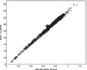
Figure 2. Plot of NAS versus references values for BRIX. Calibration (o) and Validation (+) samples.
Figure 3. Plot of NAS versus references values for POL. Calibration (o) and Validation (+) samples.
obtained for BRIX, POL and RS were ±0.60, ±0.87 and ±0.54, respectively. These results show that for BRIX and POL there are acceptable uncertainties compatible with the analytical range of the calibration models. Otherwise, for RS parameter, the CL calculated is incompatible with the concentration range studied, indicating that the proposed methodology based on NIR is not suitable for this parameter determination.
Conclusions
Determinations of BRIX, POL and RS were accessed by PLS models based on NIR spectroscopy. The models were built and validated using a representative set of samples obtaining feasible and acceptable results. The prediction errors obtained for BRIX and POL were lower than claimed at regulated norm. Confidence limits determined at the 95% confidence level for prediction samples, showed a good agreement with the expected probability of coverage. The models showed a large sensitivity capacity, differentiating samples with a low difference of concentrations. The values for accuracy, precision and other figures of merit presented promising results, indicating that the model developed by near infrared spectroscopy for BRIX and POL can be used in the sugar cane industry as an alternative to refractometry and polarization measurements (standard methods for BRIX and POL, respectively). The NIR-PLS procedure present the advantage of simpler sample preparation, since is not required that the samples of cane juice have been cleared with lead sub-acetate. Other advantages are simultaneous determination of BRIX and POL with the same NIR spectra and the possibility for on-line monitoring. For RS, using the oxidation-reduction titration method as a reference, the results of the NIR method present a better agreement than the values from the industrial equation. Therefore, the NIR method can be indicated for RS estimate in the industry, however, it should be approved for the official regulatory agency.
Acknowledgments
The authors thank COCAMAR – Cooperativa Agroindustrial for allowing the development of the experimental set-up of this work in its industrial unit. We also thank to CAPES and UNICAMP for financial support.
References
1. Shreve, R. N.; Brink Jr, J. A.; Chemical Process Industries, Mcgraw-Hill International: Auckland Bogota, 1977. 2. Payne, J. H.; Unit Operations in Cane Sugar Production,
Elsevier Science Pub. Co: Amsterdam, 1982. Figure 5. Histogram of the Student Residuals for BRIX.
Figure 6. Histogram of the Student Residuals for POL.
3. Conselho dos produtores de cana-de-açúcar, açúcar e álcool do estado do Paraná: CONSECANA-PR; Normas Operacionais de Avaliação da Qualidade da cana-de-açúcar, FAEP – Federação da Agricultura do Estado do Paraná: Curitiba, 2000. Site (URL): http://www.faep.com.br/consecana/normasop.htm, accessed in January 2004.
4. George, P. M.; Cane Sugar Handbook: A Manual for Canesugar Manufacturers and their Chemists, John Wiley & Sons Inc.: New York, London, Sydney, 1963.
5. Cadet, F.; Bertrand, D.; Robert, P.; Maillot, J.; Dieudonné, J.; Rouch, C.; Appl. Spectrosc. 1991,45, 166.
6. Cadet, F.; Robert, C.; Offmann, B.; Appl. Spectrosc. 1997,51, 369.
7. Baunsgaard, D.; Norgaard, L.; Godshall, M. A.; J. Agric. Food Chem.2000,48, 4955.
8. Johnson, T. P.; Intern. Sugar J. 2000,102, 603.
9. Irudayaraj, J.; Xu, F.; Tewari, J.; J. Food Sci.2003,68, 2040. 10. Sivakesava, S.; Irudayaraj, J.; J. Food Sci.2001,66, 972. 11. Tewari, J.; Mehrotra, R.; Irudayaraj, J.; J. Near Infrared
Spectrosc.2003,11, 351.
12. Costa Filho, P. A.; Poppi, R. J.; Proceedings of the 9th
International Conference on Near Infrared Spectroscopy, Verona, Itália, 1999.
13. Salgo, A.; Nagy, J.; Mikó, É.; J. Near Infrared Spectrosc. 1998,
6, A101.
14. Kennard, R. W.; Stone, L. A.; Technom. 1969,11, 137. 15. Burns, D. A.; Ciurczak, E. W.; Handbook of Near-Infrared
Analysis, Marcel Dekker: New York, 2001.
16. Goicoechea, H. C.; Olivieri, A. C.; Chemom. Intell. Lab. Syst.
2001,56, 73.
17. Faber, N. M.; J. Chemom.1998,12, 405.
18. Martens, H.; Naes, T.; Multivariate Calibration, Wiley: New York, 1989.
19. Faber, K.; Kowalski, B. R.; Appl. Spectrosc. 1997,51, 660. 20. Annual Book of ASTM Standards, Standard Practices for
Infrared Multivariate Quantitative Analysis - E1655-00, ASTM International, West Conshohocken: Pennsylvania, USA, 2000. 21. Lorber, A.; Faber, K.; Kowalski, B. R.; Anal. Chem.1997,69,
1620.
22. Ferré, J.; Brown, S. D.; Rius, F. X.; J. Chemom.2001,15, 537. 23. Currie, L. A.; Anal. Chim. Acta.1999,391, 105.
24. De la Pena, A. M.; Mansilla, A. E.; Valenzuela, M. I. A.; Goicoechea, H. C.; Olivieri, A. C.; Anal. Chim. Acta.2002, 463, 75.
25. Faber, K.; Kowalski, B. R.; J. Chemom.1997,11, 181. 26. Van Der Voet, H.; J. Chemom.1999,13, 195.
27. Braga, J. W. B.; Poppi, R. J.; J. Pharm. Sci.2004,93, 2124. 28. Boqué, R.; Rius, F. X.; Chemom. Intell. Lab. Syst. 1996,32,
11.
29. Boqué, R.; Larrechi, M. S.; Rius, F. X.; Chemom. Intell. Lab. Syst.1999,45, 397.
30. Boqué, R.; Faber, N. M.; Rius, F. X.; Anal. Chim. Acta. 2000,
423, 41.
31. Jarque, C. M.; Bera, A. K.; Int. Stat. Rev. 1987,55, 163.
Received: May 31, 2006
Web Release Date: February 5, 2007