Todos os direitos reservados.
É proibida a reprodução parcial ou integral do conteúdo
deste documento por qualquer meio de distribuição, digital ou
impresso, sem a expressa autorização do
REAP ou de seu autor.
The Economics of Sub-optimal Policies for Traffic
Congestion
Claudio R. Lucinda
Rodrigo M. S. Moita
Leandro G. Meyer
Bruno A. Ledo
The Economics of Sub-optimal Policies for Traffic Congestion
Claudio R. Lucinda
Rodrigo M. S. Moita
Leandro G. Meyer
Bruno A. Ledo
Claudio R. Lucinda University of São Paulo
Avenida Prof. Almeida Prado, 1280, Butantã, São Paulo /SP.
Rodrigo M. S. Moita Insper Institute
Rua Quatá, 300 – Vila Olímpia / SP.
Leandro G. Meyer University of São Paulo
Avenida Prof. Almeida Prado, 1280, Butantã, São Paulo /SP.
Bruno A. Ledo
The Economics of Sub-optimal Policies for Tra
ffi
c Congestion
⇤
Claudio R. Lucinda
†University of São Paulo
Rodrigo M. S. Moita
‡Insper Institute
Leandro G. Meyer
§University of São Paulo
Bruno A. Ledo
¶University of São Paulo
September 3, 2015
Abstract
Economic theory prescribes a (pigouvian) congestion tax in order to alleviate the negative effects of traffic congestion. It is simply a matter of internalizing a negative externality. However, traffic congestion is a pervasive problem in cities across the world, and a congestion tax is seldom applied. This paper tries to understand why this is the case. In order to do so, we estimate the welfare and traffic effects of alternative policies to be applied to the city of Sao Paulo; a congestion charge and a rotation system (or license plate restriction). With a dataset containing information on origin, destination and mode choice, we estimate a individual demand model for transportation mode. These demands are in turn used to run counter-factuals to evaluate the welfare costs of both policies. The results show that the congestion tax performs better than the rotation system in terms of aggregate welfare, but the distribution of these losses are very distinct. The congestion tax negatively affects a larger number of people with lower intensity than the rotation. Plus, the rotation system concentrates the heavier losses in an even smaller group, and thas little or no effect on driving decisions of those who owns more than one car. These results support the argument that the rotation system is chosen since it affects less people and causes little or no welfare loss on the richer portion of the population.
Keywords: urban toll; license plate restriction; urban travel demand; traffic congestion policy.
JEL Codes: L92, R41.
∗Authors would like to thank discussants to previous versions of this paper. This paper was produced as part of the research which
was conducted in the context of the research project “Urbanization and Development: Delving Deeper into the Nexus” managed by the Global Development Network (GDN). The funds for the present study were provided by the Institutional Capacity Strengthening Fund (ICSF) of the Inter-American Development Bank (IDB) as part of the IDB Initiative on Strengthening Policy Links between Latin America and Asia, and thanks to the contribution of the Government of the People’s Republic of China. The views expressed in this publication are those of the author(s) alone. Claudio Lucinda nad Rodrigo Moita gratefully acknowledges financial support from CNPq.
†Associate Professor, University of Sao Paulo at Ribeirao Preto.
‡Corresponding Author. Associate Professor, Insper Institute. Rua Quata, 300, sala 601, Sao Paulo, Brazil. CEP 04546-042.. Email: [email protected].
1
Introduction
Driving in Sao Paulo city during rush hour can be a painful experience. Congested roads with traffic gridlocks belong to the city’s daily routine. But Sao Paulo is not alone; several other cities across the world suffer from similar traffic congestion problems. Los Angeles, Singapore and Mexico City, to name a few, are famous for their congested streets and rush hour madness. This problem extrapolates to several other medium sized cities as well, where narrow streets receive an ever increasing influx of cars. Traffic congestion is a true modern world plague.
Among the consequences of traffic gridlock in urban areas there are productivity losses, increased fuel consump-tion, lowering in quality of life as well as assorted environmental effects. Such problems are even worse in major urban areas in developing countries, where adequate infrastructure is usually lacking. The number of automobiles is also a response to the insufficient supply of adequate public transportation in terms of comfort, timeliness and safety, which makes the problem even worse.
In order to try to alleviate its traffic congestion problem, Sao Paulo adopted in 1997 a circulation restriction known as “rodízio” (or “rotation”). The restriction consisted of cars with license plates terminated by 0 and 1 being prohibited to circulate around downtown on Mondays, cars with license plates terminated by 2 and 3 cannot circulate on Tuesdays, and so on. Even though this policy is in place for more than a decade, congestion is much higher now than in 1997. Mexico City adopts a similar policy, called “Hoy no Circula”. Bogota has its version of the same policy called “Pico & Placa”, among many other examples. Besides such command and control measures, cities also invest massive amounts of resources in infrastructure to try to reduce congestion.
However, such policies are not the ones economic theory would prescribe. The theory of congestion pricing has a long tradition in economics. Pioneered by the early work of Pigou [1932] and Knight [1924], it prescribes a tax - often called a pigouvian tax - to road usage. This tax would solve the problem of excess usage, bringing the traffic system to a situation of optimal allocation. In more general terms, it is simply a matter of pricing a negative externality: when a driver decides to drive on a congested road, her decision increases the travel time of other users. The social cost of road usage is greater than the private cost, and a pigouvian tax would equalize social and private cost, maximizing social welfare.
A congestion tax is seldom applied, though.1 This paper tries to understand why this is the case. In order to do so, we estimate the welfare and traffic effects of alternative policies to be applied to the city of Sao Paulo: a congestion charge, or urban toll, and a rotation system on top of existing arrangements.2 We use a dataset from the Origin-Destination survey carried out by Sao Paulo’s subway company, from which we estimate discrete choice models to identify structural parameters of individual demand for transportation modes. We then use these results to run counterfactuals to evaluate welfare impacts of both policies.
Beyond checking if the optimal policy indicated by the economic theory is indeed optimal, the interest relies more in analyzing the distribution of costs of both policies across the population, in order to have an explanation of why an optimal policy is seldom used, or at least politically difficult to implement in practice.
1
The next section of the paper describes some implementations of congestion pricing.
2
The results show that the congestion tax performs better than the rotation system in terms of aggregate welfare. However, the group that loses under the rotation system is smaller with higher losses concentrated in an even smaller share of the population, while the losses are more evenly distributed under the urban toll. Plus, the rotation has little or no effect on driving decisions of those who owns more than one car. Wealthier citizens - capable of having more than one car - can avoid the rotation system by having a “rotation’s day car”. These results support the argument that the rotation system is chosen since it affects less people and causes little or no welfare loss on the richer portion of the population.
This paper relates to a vast literature on traffic in general, and policies for traffic congestion in particular. For example, Vickrey [1969] and subsequently Arnott and DePalma [2011] analyze equilibrium conditions in a bottleneck congestion model, Souche [2010] and Albalate and Bel [2010] analyze the transportation system of a sample of cities using a supply demand setup, among many others.
Closer to this paper is the work of Gallego, Montero, and Salas [2013]. These authors analyze two policies, in Mexico City and Santiago (Chile), aimed at reducing congestion and pollution. They find the policies that impose driving restrictions may lead to a higher number of cars on the city. Our results point on the same direction. Batarce and Ivaldi [2014] estimate the demand for transportation mode taking into account traffic congestion in an equilibrium setup. In their work, traffic congestion is the equilibrium of a game with a continuum of drivers. De Borger and Proost [2012] theoretically analyze the political economy aspects of congestion pricing. Their results corroborate the emprical observation that road pricing is politically difficult to implement. We analyze the same problem empirically.
Rouwendal and Verhoef [2006] and Prud’homme and Kopp [2008] analyze and survey the use of the urban toll in different circunstances. Finally, this work builds on the classic work of McFadden [1974] and Ben-Akiva and Lerman [1985], which provide the econometric framework to analyze transportation mode choice on a discrete choice framework.
The next section will be focused on the existing restrictions in São Paulo and a short review of the international experiences on restricting the usage of private transportation. Section 3 explains the dataset used, the econometric model and estimation results. Section 4 simulates and analyze the different policies. The last section concludes.
2
International Experiences
In 2008, a report entitled “Lessons Learned from International Experience in Congestion Pricing” KTA [2008] commissioned by the U.S. Department of Transport compared the congestion pricing experiences in Singapore, London and Stockholm. Below we resume the main findings and conclusions of the mentioned report on mobility, revenue/costs, economy and business, environment and acceptability.
All of the three cities have reached their main objective of reducing congestion and keep it at lower levels. In Singapore, London and Stockholm traffic in the priced zone reduced around 10% to 30%, and that reductions were sustained over time. As consequence, the speeds increased significantly within the priced zone. In the three cities, up to 50% of those car travels through the priced zone have shifted to public transportation.
times the operating costs. In Stockholm and London the revenues have been over twice the costs. In these two cities, revenues are used mainly to recover operating and enforcement costs, although the original idea was to use revenues to improve public transportation. In Singapore, the great surplus of funds has allowed the government to implement new public transportation programs.
In general, the impacts on economy and business aspects have been neutral to positive. In Singapore, the toll did not change significantly business conditions and the community responded positively to the program. London had neutral regional economic impacts and the business communities continue to support the scheme. Finally, in Stockholm, until 2008 no significant impacts were identifiable.
The three cities have experienced a better environment as consequence of the smaller number of trips (and carbon dioxide emissions) inside the charged zone.
Public acceptance depends on all aspects listed above, and in that sense is very difficult to measure. Congestion pricing is highly controversial within the public, both before and after implementation. Stockholm minimized that controversy through a referendum. In general, the main fear of the populations is that a congestion pricing program will become just another tax.
These results indicate that the urban toll could be an alternative to the existing rotation system, if the controversy surrounding the acceptance of such measure could be avoided. In order to do so, one requirement is an estimate of the likely effects of this measure on traffic.
As mentioned, the most important Brazilian arrangement designed to reduce the automobile traffic is the so-calledRodízio, imposed by the Municipality of São Paulo in 1997 (Decree 12.490 of Oct. 3, 1997). At the time, the city government said the main reason for the Rotation was the worsening of the air quality in the city. However, a side effect (it is not clear whether it was an unintended side effect, though), was the reduction in traffic congestion right after the start of this mechanism.
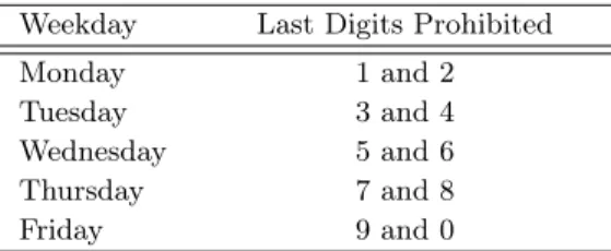
From then on, the circulation of private vehicles, excepting those of essential functions (mainly public trans-portation, school buses, ambulances and disabled persons), was prohibited in a specific area corresponding to the expanded city center, according to the last digit of the license plate, as shown in the table below:
Table 1: License Plates not Allowed to Circulate
Weekday Last Digits Prohibited Monday 1 and 2 Tuesday 3 and 4 Wednesday 5 and 6 Thursday 7 and 8 Friday 9 and 0
Source: São Paulo Traffic Company (2012).
pronounced in its first year, 1998. In 1999 the length of roads considered to be congested (that is, with traffic with a lower speed than usual) already surpassed the pre-Rotation level.
Even though the rotation system did not stop the growth of traffic gridlock, this system was essentially unchanged from 1997 to the present day. These policies strongly affect the daily life of the city, and can be very unpopular at first.3
Both the international experiences and the analysis of the Brazilian case indicate public acceptance of any policy aimed at restricting traffic is an essential ingredient to any policy being enacted. Since our goal is to investigate winners and losers from two alternative policies, the next step is to carry out estimation of structural demand parameters.
3
Empirical Analysis
3.1
Data
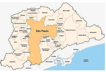
The main source of transportation statistics to be used will be the Origin-Destination (OD) survey carried out by the São Paulo Subway Company. This survey has 169,625 observations, with information about trips made in 2007 in the region composed by 38 municipalities besides São Paulo city, depicted in Figure 1, an area known as Metropolitan region of São Paulo marked in yellow (38 municipalities) and in orange (São Paulo city).
In this survey, detailed information on the origin, destination, mode choice and attributes (both individual and chosen transportation mode) were recorded. The survey was carried out by a team of 370 researchers, visiting 54,700 households, with approximately 30,000 of those considered valid after the vetting process of the raw data. The Survey uses a stratified sampling technique, with error margins below 5%.
3
Figure 1: São Paulo Metro Area
Source: OD Survey, São Paulo (2007).
The survey has a wide range of individual information, such as income, car and home ownership, household size and other characteristics which could influence the decision of whether or not to take the trip and what transportation mode to use. The survey also has trip information as departure and arrival time, latitude and longitude for departure and arrival, mode transportation, reason of the trip – leisure or work – and so on.
Some preliminary analyses were made regarding trip features and the characteristics of the individuals. The results are presented below.
Figure 2: Trip distribution during the day
0
5000
1.0e+04
1.5e+04
2.0e+04
Frequency
0 5 10 15 20 25 hora da saída
Departure time
0
5000
1.0e+04
1.5e+04
2.0e+04
Frequency
0 5 10 15 20 25 hora da chegada
Arrival time
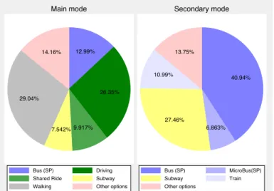
The trips are concentrated mainly during three periods of the day, between 6 and 9 AM, between 12AM and 1PM (about lunchtime) and between 5PM and 7PM, determining the peak hours for usage of urban road infrastructure. One important feature of the trips is that some individuals may use more than one transportation mode. Among the 169,625 trips related in the survey, 21,304 (12.6%) are made with more than one transportation mode: 17,313 (10.2%) individuals use two, 3,627 (2.1%) use three and 364 (0.2%) use four modes. The share of each transportation mode used as principal and secondary modes are shown in the Figure 3.
Figure 3: Share of transportation mode (main and secondary mode)
12.99%
26.35%
9.917% 7.542% 29.04%
14.16%
Bus (SP) Driving
Shared Ride Subway
Walking Other options
Main mode
40.94%
6.863% 27.46%
10.99% 13.75%
Bus (SP) MicroBus(SP)
Subway Train
Other options
Secondary mode
Source: OD Survey, São Paulo (2007).
The figure shows that car is the most used transportation mode, with driving and shared ride summing 36.15% of the trips. Walking is also a very important main mode, with 29.30%. This happens because an important part of the sample is constituted by short trips – trips shorter than 2 km sum 44.22% of the sample.
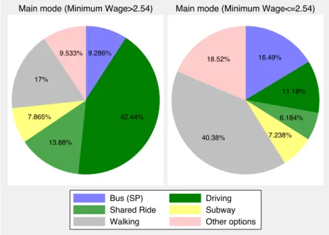
Figure 4: Main transportation mode for families with minimum wage above and below the sample mean
9.286%
42.44%
13.88% 7.865%
17% 9.533%
Main mode (Minimum Wage>2.54)
16.49%
11.18%
6.184%
7.238% 40.38%
18.52%
Main mode (Minimum Wage<=2.54)
Bus (SP) Driving
Shared Ride Subway
Walking Other options
Source: OD Survey, São Paulo (2007).
The share of car trips (driving and shared ride) in the group with higher income is 56.14% and in the group with smaller income is 17.32%. The opposite occurs if we consider the walking option, which share is 17.26% in the richer group and grows to 40.53% in the poorer. A similar pattern is observed for the bus alternative, which increases from 9.25% to 16.41% from the richer to the poorer group. The share of subway usage is similar in both groups.
Another important division of the zones is the Expanded Center (EC) of São Paulo City. Since it is the part of the city where the restriction to traffic is applied, it is important to study specifically this area.
The EC is composed by 17 of the total of 460 zones in which the survey was carried out and it is located right in the center of São Paulo city. This region has a very intense economic activity and therefore it is expected to have the most intense traffic.
Driving is the more frequent transportation mode used to or from the expanded center. Almost half of the individuals that use car go or come from the expanded center, which may be one of the reasons of the that increase traffic in the region. Regarding the public transportation modes, subway is more frequently used to go to the expanded center than bus.
Since the EC is related to a very important part of the trips in the survey and it is the zone in which the current traffic restrictions are imposed, it is important to analyze some features of this region.
travels related to the EC.
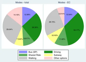
Figure 5: Modes of transportation for all sample and for trips related to expanded center (2007)
12.99%
26.35%
9.917% 7.542% 29.04%
14.16%
Modes - total
12.54%
34.17%
11.62% 8.918% 26.73%
6.014%
Modes - EC
Bus (SP) Driving
Shared Ride Subway Walking Other options
Source: OD Survey, São Paulo (2007).
Driving and shared ride sum 36.1% in the sample, but considering only the trips related to the EC this sum increases to 45.6%. The other modes have similar shares in both groups.
This part of the descriptive analyses implies that, even with the actual restriction to usage of private vehicles, driving and shared rides are the most important options in trips related to the EC, which shows the importance of restrictions on usage of individual transportation modes in this part of the city.
To sum up, the characteristics above point out to the EC being an important trip origination and destination region, especially for automobiles, despite being subject to the traffic restrictions discussed in the previous section. These points indicate the EC should be a natural choice for further traffic policies.
3.2
Travel Costs
The most relevant data which is not available in the OD survey is trip cost. A different methodology was used for imputing costs for each trip, and they are described below. We assume some modes - such as walking, shared ride and bike - to have zero monetary costs.
3.2.1 Car
To estimate the cost of car trips we used the following formula:
T C=⇥d
t/dg
⇤
⇥pg⇥t
In which d is trip distance, t trip time, g gasoline consumption and pg is gasoline price. Since the distances
hour, which multiplied by the travel time and by the gasoline price equals the trip cost. The average speed is calculated for some hours during the day by the Traffic Engineering Company of São Paulo (CET) annually. In the year of 2007, the average speed was 17 km/hour between 5AM and 8AM hours and 14.2 km/hour between 5PM and 7PM. In order to obtain the average speed in other periods of the day, the average speed for all periods for the trips of the OD were calculated. Then, the relationship between the values available in the CET research and the values calculated with the OD data was used to calculate the average speed for the remaining periods (between 12AM and 1PM and the rest of the day).
The relationship between distance and gasoline usage is calculated since 2009 for a range of the most popular cars in Brazil by the National Institute of Metrology, Quality and Technology (INMETRO) . These relationships were weighted by the number of each car model sold in São Paulo state between 2002 and 2007, data available by the National Association of Automobile Retailers (FENABRAVE).
The mean gasoline price in São Paulo for each month of 2007 is available by the National Agency of Petroleum, Natural gas and Biofuels (ANP). The travel time is available at the OD survey, computed as the difference between departure and arrival time.
3.2.2 Motorcycle
The same formula was applied. The only difference between the cost of motorcycle and car trips is the ratio between distance and the gasoline usage. In the case of motorcycle, this number was calculated by the weighted mean of the fuel efficiency of the seven models of motorcycle more common in the Brazilian roads, which sum 81.5% of the total motorcycles. The efficiency is available in specialized websites.
3.2.3 Inter municipal bus
There are three bus types recorded in the dataset: (i) Municipal buses, which have their billing systems integrated with subway and rail systems and have the same fare, in a system called bilhete único, (ii) Intermunicipal buses, which make trips between different municipalities in São Paulo metropolitan area and have their prices set by a São Paulo state level agency (EMTU) and (iii) buses for hire, which are quite common for work trips to the main business districts in São Paulo. The price of intermunicipal bus trips are available in the Metropolitan Urban Transports Enterprise of São Paulo (EMTU) web site.4 In some cases, there are di
fferent prices for the same trip. In such cases, the mode of the relevant prices was considered. In the cases in which this criterion resulted in more than one value, the lower one was considered.
Not all trip prices were available for 2007. In these cases, 2012 prices were discounted by the ratio between the mean prices of 2007 and 2012 for each region. However, there were cases in which the trip in the OD did not have a correspondent price in the EMTU website. In such cases the price considered was the mean trip price from the same city.
4
3.2.4 Subway, train and municipal bus
According to the Metropolitan train company of São Paulo, subway, train and municipal bus fares in 2007 was BRL 2.30.
3.2.5 Hired bus
The trip price for hired buses was calculated considering BRL 1.4/km divided by 10, which is the number of passengers considered. The BRL 1.4 figure was determined after consultation with one of the most important bus companies.
3.2.6 Taxi
Taxi fares for hours of trip in the year of 2007 was available at the website of São Paulo municipality.
3.2.7 Final Choice Set
From these trip prices and costs, we reduced the choice set to the following set of alternatives:
• Bus: trips that respondents answered as their main mode choice either municipal, intermunicipal or hired buses
• Rail: trips that respondents answered as main mode choice as subway or rail.
• Driving: trips that respondents answered as main mode choice as driving
• Motorcycle: trips that respondents answered as main mode choice as motorcycle
• Taxi: trips that respondents answered as main mode choice as taxi
• Other: other main mode choices - usually shared ride, walking or bicycle.
3.3
Travel time and cost matrices
Another important part of the database preparation is computing time and cost of options that were available but not chosen by the decision maker. Some alternatives had costs that could be determined the same way as costs for trips actually made – such as bus, subway and rail trips. For the other alternatives, the costs and duration for the other choices were estimated from a regression model using the observed choices for each mode. The dependent variable was the logarithm of trip cost or trip duration, and the independent variables were as such:
• Dummy Variables for Departure Hour
• Dummy Variables for Trip Motivation
• Distance in kilometers
The latter variable was estimated as the Euclidean Distance between the geographical coordinates of the OD zones (according to the survey’s division in 460 zones). The estimated coefficients were used to estimate expected trip time and cost for alternatives not chosen.5
Not all modes were available to all respondents, though. This problem was more pronounced for rail and subway modes, given the lack of infrastructure for all zones. This problem was addressed by restricting the availability of rail and subway choices for only those zones which had some respondents choosing these modes.
Given this dataset, the next section will be focused on the modeling to be used.
3.4
Econometric Analysis
In this section, we discuss our econometric approach. More specifically, we present the mixed logit model (see Train [2009], for a full discussion of this class of models), although the analysis is also carried out for the multinomial logit.6 The mixed logit approach is used here because it can provide more flexible substitution patterns than both the multinomial logit and the nested logit – for instance, used by Molnar and Mesheim [2010]. The starting point is a population ofN potentially heterogeneous individuals, so letsn be the vector of characteristics for an individual
member of this population denotedn. Each individual have to decide which transportation mode to take to work. From the choice set defined above, it is assumed the respondents must choose a single alternative from a subset of the discrete choice setJ ={Bus, Rail, Driving, Motorcycle, Taxi, Other}– which may include all of them, but not all alternatives must be available to all individuals.
For each i 2 J alternative, individual n derives utility Uni. Assuming that individual’s behavior is
utility-maximizing, choices can be represented by a binary variable defined as:
yni=
8 < :
1 ifUni> Uni08i6=i0
0 otherwise (1)
Individual choices depend on many factors that may affect their utility from each alternative, either because of differences in individual characteristics that may affect the desirability of each alternative in a different way or because of differences in characteristics of alternatives. Assuming the utility can be decomposed into two parts: one part deterministic and other random, one can writeUnias:
Uni=βnizni+εni (2)
5
Results available upon request.
6
In which zni is a set of observed variables relating to alternativeifor individual n that depends on attributes
of the alternative xni, interacted perhaps with attributes of the individual, sn, such that it can be expressed as
zni = z(xni, sn) for some numerical function z. It is assumed here the function z is the identity, which makes
zni= [xni:sn].
• βniis a corresponding vector of coefficients of the observed variables, and
• εni captures the impact of all unobserved factors that affect the individual’s choice.
Whenεni follows an extreme-value distribution, we say that it belongs to the Generalized Extreme Value (GEV)
family of models [Fisher and Tippett, 1928, Gnedenko, 1943]. In both the multinomial and mixed logit models the stochastic termεnifollows an extreme-value distribution.
The multinomial logit (MNL) model is the most basic member of the family of GEV models, with the well known choice probability formula for individualnand alternativei:
Pni=
exp[βnizni]
PJ
j=1exp[βniznj]
(3)
In which J is the total number of alternatives.
The MNL model is the mostly commonly used in discrete choice analysis, however it assumes that there is no correlation inεinover alternatives. This lack of correlation results in a property known as Independence of Irrelevant
Alternatives (IIA). The IIA property implies that MNL model “cannot account for choice situations where a new alternative more than proportionately reduces the choice probabilities of existing alternatives that are similar, while causing less than proportionate reductions in the choice probabilities of dissimilar alternatives” [Anderson et al., 1992]. A number of models have been proposed to allow correlation over alternatives and avoid the IIA property, such as the Nested Logit of Molnar and Mesheim [2010]. Here we use the mixed logit.
The solution to the IIA problem by the mixed logit does not depend on an a priori nesting structure. It is assumed, under this model, that the coefficients have some sort of heterogeneity – either related to observed characteristics or to unobserved characteristics. Adapting the previous notation, the utility for consumer n of choosing alternativei as follows:
Uni=βnizni+σvnzni+εni
In whichσ is a vector capturing heterogeneity in (possibly some of) theβ parameters, andvn is an additional
random perturbation (which would be related to observed variables or unobserved ones). Still assuming a GEV distribution for theεniterm, the choice probability for alternativei could be derived for individualn:
Pni=
ˆ exp[β
nizni+σvnzni]
PJ
j=1exp[βniznj+σvnznj]
This formula is somewhat different from its MNL analogue because of the integral required to account for the random nature of thevn terms. Depending on the assumed distribution, which is denoted byP(v)in the previous
formula, the integral for the choice probability could be computed numerically (by some sort of quadrature method), or by simulation. In the present paper the relevant integrals – assuming a standard normal distribution for the v terms – are estimated by simulation, using 50 Halton draws. These simulated choice probabilities are used to estimate theβniandσ parameters by Maximum Likelihood.
Closed forms can also be derived for the Equivalent Variation, which will be used to compute the effects of counter-factual measures, such as the urban road tax discussed here. The consumer surplus is approximated by the so-called logsum measure [Small and Rosen, 1981]:
E(CS) =
ˆ ln
h PJ
j=1exp[βznj+σvnznj]
i
α dP(v) +C (5)
In which α represents the marginal effect of the cost variable on the non-random part of utility, and C is an integration constant which will be ingored throughout the analysis
The empirical implementation of the model requires some definition of the relevant variables to be used. As for alternative specific variables composing thexnisubset of variables, Trip Cost and Trip Time were used, as well as
the ratio of trip cost to income as well as trip time to income. For case specific variables, the ones selected were:
• Age
• Income in 1000BRL
• Dummies for:
– Female Gender
– Student
• Dummy if the Trip is during Peak Hours
• Dummy if there are easy connecting routes between bus and rail
• Dummy if there are dedicated bus lanes in the trip origin
the ratio of Trip Time to Income in 1000 BRL. This specification leads to the following function for theαterm in equation (5):
α=βT C+
βT C|I
IN C +σT Cvn
The second technical issue to be faced pertains to the normalization restrictions required to identify the model. The first one is a variance restriction on the εni term on the random part of utility. And the second one is the
normalization on coefficiens of individual characteristics, which were normalized to zero for the base alternative. The utility level for the base alternative becomes, then:
Un0=βT CT Cn0+
βT C|I
IN Cn
T Cn0+σT Cvn+βT CT Tn0+
βT T|I
IN Cn
T Tn0+σT Tvn
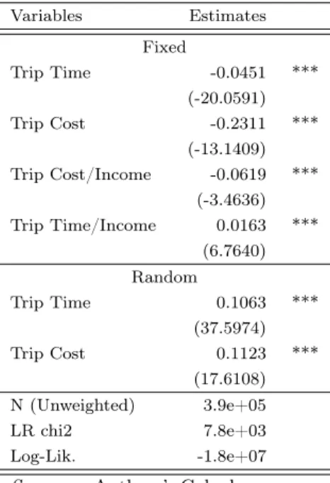
The results for the marginal effects of trip cost, trip time and their interaction with income are in Table 2.
Table 2: Mixed Logit Results – Trip Cost and Trip Time Variables
Variables Estimates
Fixed
Trip Time -0.0451 *** (-20.0591) Trip Cost -0.2311 ***
(-13.1409) Trip Cost/Income -0.0619 ***
(-3.4636) Trip Time/Income 0.0163 ***
(6.7640) Random
Trip Time 0.1063 *** (37.5974) Trip Cost 0.1123 ***
(17.6108) N (Unweighted) 3.9e+05 LR chi2 7.8e+03 Log-Lik. -1.8e+07
Source: Authors’ Calcula-tions. * p<0.05, ** p<0.01, *** p<0.001
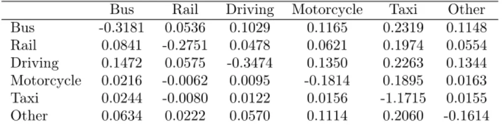
The cost elasticities are presented in Table 3 below7.
Table 3: Estimated Mean Elasticities for Work Trips
Bus Rail Driving Motorcycle Taxi Other
Bus -0.3181 0.0536 0.1029 0.1165 0.2319 0.1148
Rail 0.0841 -0.2751 0.0478 0.0621 0.1974 0.0554
Driving 0.1472 0.0575 -0.3474 0.1350 0.2263 0.1344
Motorcycle 0.0216 -0.0062 0.0095 -0.1814 0.1895 0.0163
Taxi 0.0244 -0.0080 0.0122 0.0156 -1.1715 0.0155
Other 0.0634 0.0222 0.0570 0.1114 0.2060 -0.1614
Elasticities are in line to the results of Molnar and Mesheim [2010] and Gagnepain, Ivaldi, and Vibes [2011], with the latter mentioning a value of -0.4 for a trip cost elasticity for bus trips. The one estimated here is -0.3181, a bit lower in absolute value than the -0.4 of Gagnepain, Ivaldi, and Vibes [2011], and much closer to the results in the range of -0.3 to -0.4 of Molnar and Mesheim [2010].
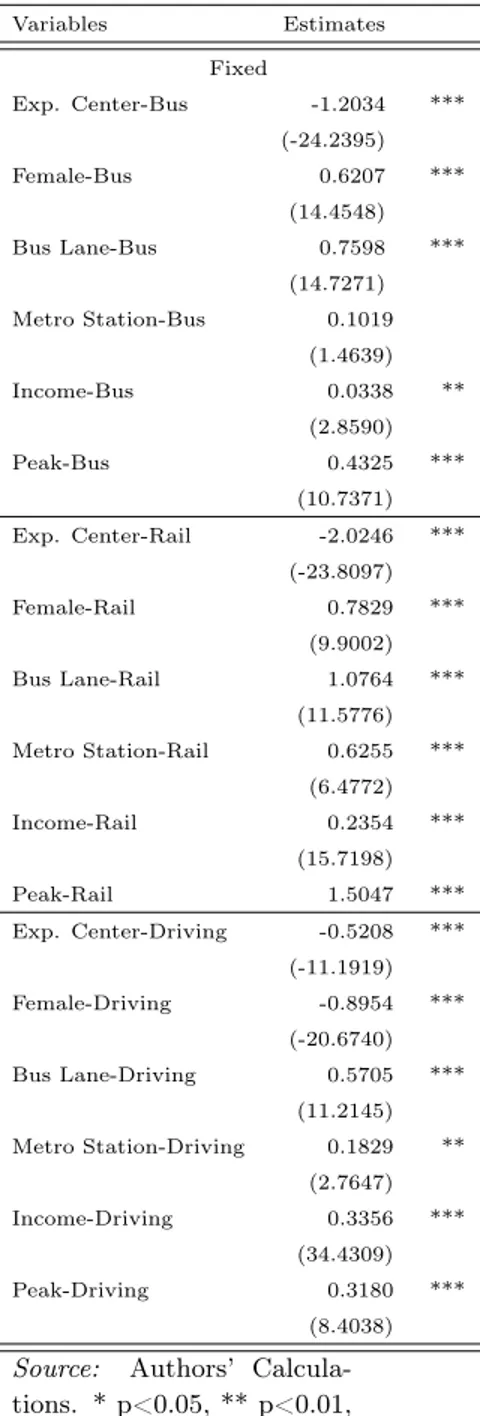
The effects of individual and route characteristics on Bus, Rail and Driving choices – the most important ones – are presented in Table 4 below:
7
Table 4: Mixed Logit Results - Driving, Bus and Rail
Variables Estimates
Fixed
Exp. Center-Bus -1.2034 ***
(-24.2395)
Female-Bus 0.6207 ***
(14.4548)
Bus Lane-Bus 0.7598 ***
(14.7271)
Metro Station-Bus 0.1019
(1.4639)
Income-Bus 0.0338 **
(2.8590)
Peak-Bus 0.4325 ***
(10.7371)
Exp. Center-Rail -2.0246 ***
(-23.8097)
Female-Rail 0.7829 ***
(9.9002)
Bus Lane-Rail 1.0764 ***
(11.5776)
Metro Station-Rail 0.6255 ***
(6.4772)
Income-Rail 0.2354 ***
(15.7198)
Peak-Rail 1.5047 ***
Exp. Center-Driving -0.5208 ***
(-11.1919)
Female-Driving -0.8954 ***
(-20.6740)
Bus Lane-Driving 0.5705 ***
(11.2145)
Metro Station-Driving 0.1829 **
(2.7647)
Income-Driving 0.3356 ***
(34.4309)
Peak-Driving 0.3180 ***
(8.4038)
Source: Authors’ Calcula-tions. * p<0.05, ** p<0.01, *** p<0.001
and increases the choice probability for bus and rail. As for infrastructure availability, both the availability of a Metro Station and Dedicated Bus Lanes increase the choice probability of using Rail and Driving for the trip. The availability of a dedicated bus lane increases the probability of a trip being made using bus, but the availability of a metro station does not have any impact on the choice probability of a bus trip, compared to the outside alternative. From the estimated parameters, the policy simulations will be carried out, and their results will be discussed in the next section
4
Policy Analysis
In this section, we analyze the welfare impacts of two policies calibrated to achieve the same end result: a 33% in traffic reduction. They are:
1. An extension of the existing rotation system, in which 50% of the existing cars are not allowed to circulate through the expanded center on a given day, and violating the legislation implies in a penalty of 128 BRL (40 US Dollars).
2. The imposition of an urban toll of 3.5 BRL per trip.
The numbers used in alternatives (1) and (2) were selected as to generate a 33% decrease in driving in the expanded center in both cases. By equating benefits across alternatives, we are able to compare the costs associated with each alternative.
The implementation details of both alternatives also merit some explanation. For the expanded rotation, an uniform random variable bounded between zero and one was generated for each individual who owns a car and if the random draw was below 0.5, then it was deemed eligible for the rotation and the cost of driving to/from the expanded center was increased by the amount of the fine, 128 BRL. Indivduals who own two cars were under the rotation system if his draw was under 0.25 and so on: citizens with more than one car have a higher chance of bypass the rotation system.
For the urban toll, the trip cost for driving to/from the expanded center was increased by 3.5 BRL. Both policies were simulated for two days, such that all plates were once under the rotation, and the welfare effects were calculted based on the sum of these two days.
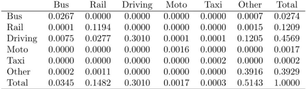
Table 5: Changes in Traffic Flows - Work Trips under Congestion Charge
Bus Rail Driving Moto Taxi Other Total
Bus 0.0267 0.0000 0.0000 0.0000 0.0000 0.0007 0.0274
Rail 0.0001 0.1194 0.0000 0.0000 0.0000 0.0015 0.1209
Driving 0.0075 0.0277 0.3010 0.0001 0.0001 0.1205 0.4569
Moto 0.0000 0.0000 0.0000 0.0016 0.0000 0.0000 0.0017
Taxi 0.0000 0.0000 0.0000 0.0000 0.0002 0.0000 0.0002
Other 0.0002 0.0011 0.0000 0.0000 0.0000 0.3916 0.3929
Total 0.0345 0.1482 0.3010 0.0017 0.0003 0.5143 1.0000
Table 6: Changes in Traffic Flows - Work Trips under Rotation System
Bus Rail Driving Moto Taxi Other Total
Bus 0.0270 0.0000 0.0000 0.0000 0.0000 0.0004 0.0274
Rail 0.0000 0.1201 0.0000 0.0000 0.0000 0.0008 0.1209
Driving 0.0057 0.0183 0.3071 0.0001 0.0000 0.1258 0.4569
Moto 0.0000 0.0000 0.0000 0.0017 0.0000 0.0000 0.0017
Taxi 0.0000 0.0000 0.0000 0.0000 0.0002 0.0000 0.0002
Other 0.0001 0.0007 0.0000 0.0000 0.0000 0.3921 0.3929
Total 0.0328 0.1391 0.3071 0.0018 0.0002 0.5191 1.0000
They also have similar patterns of traffic shifting, with a small share of drivers migrating to rail, and a larger fraction choosing Other, meaning walking, riding a bike etc.
The welfare effects of both policies are shown next. The congestion tax imposes a smaller loss than the rotation system. Note that they are both welfare reducing since we are simulating only the cost of each policy.
Table 7: Welfare Measures
Original Tax Rotation
Mean 10.6245 8.3471 7.0466
Total 2.9e+05 2.3e+05 1.9e+05
Table 8: Consumer Surplus Loss - Statistics
obs mean var total
Rotation 120555.0 -5.9 34.1 -7.1e+05
Tax 165638.0 -2.7 3.3 -4.4e+05
This point is taken further in Table 9, where the quantiles of the losses’ distribution are presented. The lowest percentile in terms of losses need to have an income increase of 27.4 BRL to be indifferent between the status quo and the expanded rotation, whereas the lowest percentile in terms of losses for the Urban Tax need only to have an increase in income of 6.80 BRL.
Table 9: Consumer Surplus Loss - Quantiles
1st 5th 10th 25th 50th 75th 90th 99th
Rotation -27.4 -17.0 -12.8 -7.6 -4.2 -2.1 -1.0 -0.1
Tax -6.8 -6.2 -5.5 -3.9 -2.3 -1.2 -0.5 -0.1
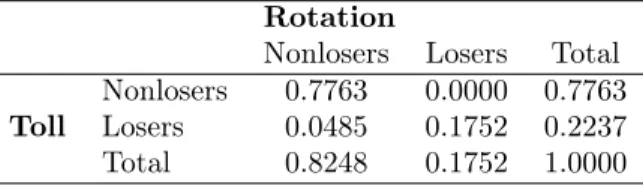
Besides the distribution of losses, one might be interested in whether the individuals who lose in each policy are the same. The results of Table 10 indicate that more than 77% of all individuals do not lose under both policies and 17% lose under both policies. Only 4.85% of individuals do not lose under the rotation system and lose under the urban toll, indicating it is not different groups trying to shift losses are responsible for one instead of other policy.
Table 10: Losers - Urban Toll (row) vs Rotation (column)
Rotation
Nonlosers Losers Total
Toll
Nonlosers 0.7763 0.0000 0.7763
Losers 0.0485 0.1752 0.2237
Total 0.8248 0.1752 1.0000
To further characterize the population affected by the policies, we regressed a dummy variable that indicates if the person loose utility under the policy on the person and route characteristics. The results are shown in Table 11. This table basically says that the higher income population, which happens to live on neighborhoods with metro stations and dedicated bus lanes are the ones affected by the policy.8
A straightforward question at this point is; why does the rotation system affect less people than the urban toll? The answer relys on the second (or third, fourth...) car. The infamouscarro do rodizio (rotation day’s car). Tables 12 and 13 show the proportion of people affected by the policies, urban toll and rotation respectively, conditional on the number of cars owned.
8
Table 11: Who are the losers?
Tax Rotation
Exp. Center 0.3736 *** 0.2870 ***
(115.6672) (84.3997)
Female -0.0164 *** -0.0083 **
(-5.7907) (-2.7726)
Bus lane 0.0933 *** 0.0840 ***
(30.2710) (25.8820)
Metro station 0.1003 *** 0.0891 ***
(26.5118) (22.3811) Income in 1000BRL 0.0403 *** 0.0098 ***
(102.3978) (23.6269)
Peak -0.0011 -0.0015
(-0.8732) (-1.1772)
Constant 0.0647 *** 0.1098 ***
(21.4439) (34.5437)
Observations 7.9e+04 7.9e+04
Log-Lik. -3.9e+04 -4.3e+04
* p<0.05, ** p<0.01, *** p<0.001
Obviously, non car owners are not affected at all, and the proportion of owners of one car affected is the same under both policies. The differences appear when we look at individuals who have more than one car. The congestion tax affects 50% more people that owns two cars than the rotation. In fact, the rotation has only a negligible effect on the owners of two or more cars.
Table 12: Losers and car ownership - Tax
0 1 2 3 4 Total
Nonlosers 0.3952 0.2741 0.0810 0.0148 0.0114 0.7763
Losers 0.0020 0.1409 0.0596 0.0117 0.0094 0.2237
total 0.3972 0.4150 0.1406 0.0265 0.0208 1.0000
With these dataset, we cannot say the rotation in place nowadays in Sao Paulo induced the purchase of these extra cars. However, this is evidence that the incentive to do so exists. This result is in line with the findings of Gallego, Montero, and Salas [2013], in which policies imposing driving restrictions may lead to a larger stock of cars.
5
Conclusions
Table 13: Losers and car ownership - Rotation
0 1 2 3 4 Total
Nonlosers 0.3972 0.2741 0.1108 0.0227 0.0200 0.8248
Losers 0.0000 0.1409 0.0298 0.0038 0.0008 0.1752
total 0.3972 0.4150 0.1406 0.0265 0.0208 1.0000
Hoy no Circula, Pico & Placa etc) - are more commonly observed than the congestion pricing. To analyze this question, this paper estimates the demand for urban transportation mode choice and simulate two traffic reduction policies, urban toll and rotation system, to perform a welfare analysis.
Confirming economic theory’s prediction, the aggregate results show that the urban toll is welfare superior to the rotation system. But a closer look at the welfare consequences of these policies reveal other things. First, despite generating a smaller welfare loss - on aggregate and on average - the urban toll affects more peolple than the rotation system. Second, the distribution of losses under the rotation system is even more skewed, meaning that there is a small group who gets an over proportional share of the policy’s burden. And third, the difference in the fraction of the population affected by both policies is due to the fact that wealthier citizes avoid the rotation by having a second car, or the “rotation’s day car”. This last result shows a side effect of the rotation system, that is to provide incentives for people to buy cars. It is an undesireable side effect.
Despite being more efficient, we find evidence that the allocation of costs of an urban toll makes it politically more difficult to implement. It affects more people more evenly, while the rotation concentrated losses on a smaller group, with little effect on the wealthier citizens.
References
Daniel Albalate and Germa Bel. Tourism and urban public transport: Holding demand pressure under supply constraints. Tourism Management, 31(3):425–433, 2010.
Simon Anderson, Andre de Palma, and Jacques-Francois Thisse.Discrete Choice Theory of Product Differentiation. MIT Press, Cambridge, 1992. ISBN 026201128X.
Richard Arnott and Elijah DePalma. The corridor problem: preliminary results on the no-toll equilibrium. Trans-portation Research Part B: Methodological, 45(5):743–768, 2011.
Marco Batarce and Marc Ivaldi. Urban travel demand model with endogenous congestion. Transportation Research Part A: Policy and Practice, 59:331–345, 2014.
BBC News. Congestion charge leads to budget shortfall, June 2012. URL \url{http://news.bbc.co.uk/2/hi/
uk_news/england/london/2985554.stm}.
Gary Chamberlain. Multivariate regression models for panel data. Journal of Econometrics, 18(1):5–46, 1982.
F. F. Costa. 2007.
Bruno De Borger and Stef Proost. A political economy model of road pricing. Journal of Urban Economics, 71(1): 79–92, 2012.
C. Ferraz and P. A. Szasz. Technical report, 2005.
Ronald Aylmer Fisher and Leonard Henry Caleb Tippett. Limiting forms of the frequency distribution of the largest or smallest member of a sample. InMathematical Proceedings of the Cambridge Philosophical Society, volume 24, pages 180–190. Cambridge Univ Press, 1928.
Philippe Gagnepain, Marc Ivaldi, and Catherine Vibes. A handbook of transport economics, chapter The industrial organization of competition in local bus services, pages 744–762. Edward Elgar, 2011.
Francisco Gallego, Juan-Pablo Montero, and Christian Salas. The effect of transport policies on car use: Evidence from latin american cities. Journal of Public Economics, 107:47–62, 2013.
B. Gnedenko. Sur La Distribution Limite Du Terme Maximum D’Une Serie Aleatoire. The Annals of Mathematics,
44(3):423+, July 1943. ISSN 0003486X. doi: 10.2307/1968974. URLhttp://dx.doi.org/10.2307/1968974.
A. R. Hole. MIXLOGIT: Stata module to fit mixed Logit models by using maximum simulated likelihood. Statistical Software Components s456883, Boston College, Department of Economics, 2007. revised 18 Oct 2010.
M. Iglesias. Estimation of home-based social/recreational mode choice models. Technical report, Technical Re-port HBSRMC (n.1), Planning Section, Metropolitan TransRe-portation Commission, 101 Eight Street, Oakland, California, 1997.
Frank H Knight. Some fallacies in the interpretation of social cost. The Quarterly Journal of Economics, pages 582–606, 1924.
F. S. Koppelman and C. Bhat. A self instructing couse in mode choise modeling: Multinomial and nested logit models. Technical report, U.S. Department of Transportation Federal Transit Admnistration, 2006.
F.S. Koppelman. Multidimensional model system for ntercity travel choice behavior. Transportation Research Record, 1241:1–8, 1989.
KPMG Peat Marwick in association with ICF Kaiser Engineers, Inc. Midwest system sciences, resource systems group, comsis corporation and transportation consulting group florida high speed and intercity rail market and ridership study: Final report. Technical report, Florida Department of Transportation, 1993.
KTA. Lessons learned from international experience in congestion pricing. Report, August 2008. URL http:
K.T. Lawton. Travel forecasting methodology repory. Technical report, Metropolitan Service District, Portland, OR, 1989.
R Duncan Luce and Patrick Suppes. Preference, utility, and subjective probability. Handbook of mathematical psychology, 3:249–410, 1965.
N.L. Marshall and K.Q. Ballard. New distribution and mode choice models for the chicago region. InAnnual TRB Meeting, Washington, D.C., January 1998.
Daniel McFadden. The measurement of urban travel demand. Journal of public economics, 3(4):303–328, 1974.
Jozsef Molnar and L Mesheim. A disaggregate analysis of demand for local bus service in great britain (excluding london) using the national travel survey.Draft, University College London and Institute for Fiscal Studies, 2010.
J. D. Ortuzar and L. G. Willumsen. Modelling transport. Wiley-Blackwell, Oxford, 2011. ISBN 0470760397.
Arthur C. Pigou. The Economics of Welfare. Macmillan and Co., London, 1932.
Remy Prud’homme and Pierre Kopp. Road Congestion Pricing In Europe: Implications for the United States,
chapter Worse than a congestion charge: Paris traffic restraint policy, pages 252–265. Edward Elgar, 2008.
C.L. Purvis. Disaggregate estimation and validation of a home-based work mode choice model,. Technical report, technical report HBWMC (n.2), Planning Section, Metropolitan Transportation Commission, 101 Eight Street, Oakland, California, 1997.
Jan Rouwendal and Erik T Verhoef. Basic economic principles of road pricing: From theory to applications.
Transport policy, 13(2):106–114, 2006.
Singapore Land Transport Authority. What is electronic road pricing. URL http://web.archive.org/web/
20080921090813/http://www.lta.gov.sg/motoring_matters/index_motoring_erp.htm.
Kenneth A. Small and Harvey S. Rosen. Applied welfare economics with discrete choice models. Econometrica, 49(1):105–30, January 1981.
Stephanie Souche. Measuring the structural determinants of urban travel demand. Transport policy, 17(3):127–134, 2010.
Swedish Transport Agency. Congestion tax in stockholm. URLhttp://www.transportstyrelsen.se/en/road/
Congestion-tax/Congestion-tax-in-stockholm/.
Kenneth Train.Discrete choice methods with simulation. Cambridge University Press, Cambridge New York, 2009. ISBN 0521747384.
Transport for London. Annual report and statement of accounts 2006/07. Report, April 2007a. URL http:
Transport for London. Congestion charge (official). URL http://www.tfl.gov.uk/roadusers/ congestioncharging/.
Transport for London. Impacts monitoring, fifth annual report. Report, June 2007b. URLhttp://www.tfl.gov.
uk/assets/downloads/fifth-annual-impacts-monitoring-report-2007-07-07.pdf.
William S. Vickrey. Congestion theory and transport investment. The American Economic Review, 1969.
Alan A. Walters. The theory and measurement of private and social cost of highway congestion. Econometrica, 1961.
A
Descriptive Statistics
Table 14: Descriptive Stats
N mean max min sd
Trip Cost 8.69e+05 6.456 4786.215 0.000 17.368
Trip Time 8.69e+05 38.683 29733.650 1.000 73.608
Income in 1000BRL 6.28e+05 1.145 40.000 0.000 2.088
Age 8.69e+05 34.891 97.000 1.000 18.610
Female 8.69e+05 0.507 1.000 0.000 0.500
Student 8.69e+05 0.684 1.000 0.000 0.465
HH Size 8.69e+05 3.867 24.000 1.000 1.844