Applying distance metrics for anomaly detection of energy-based attacks in IoT sensors
Aplicação de métricas de distancias para detecção por anomalia de ataques baseados em
energia em sensores IoT
DOI:10.34117/bjdv6n11-595
Recebimento dos originais: 27/10/2020 Aceitação para publicação: 27/11/2020
André Proto
Doutorando em Engenharia de Computação Escola Politécnica da Universidade de São Paulo
Departamento de Engenharia de Computação e Sistemas Digitais LASSU – Laboratório de Sustentabilidade
Endereço: Av. Professor Lúcio Martins Rodrigues, Travessa 4, n° 380, 2° andar CEP 05508-020 - Cidade Universitária - São Paulo SP – Brasil
E-mail: andre.proto@usp.br
Tereza Cristina Melo de Brito Carvalho
Professora Associada da Escola Politécnica da Universidade de São Paulo Doutora em Engenharia Elétrica
Escola Politécnica da Universidade de São Paulo
Departamento de Engenharia de Computação e Sistemas Digitais LASSU – Laboratório de Sustentabilidade
Endereço: Av. Professor Lúcio Martins Rodrigues, Travessa 4, n° 380, 2° andar CEP 05508-020 - Cidade Universitária - São Paulo SP – Brasil
ABSTRACT
Internet of Things (IoT) has gained significant mindshare in academia and industry over the years. It is usually composed of tiny devices/sensors with low processing, memory, and energy available. As an emerging technology, many open challenges about the security of those devices are described in the literature. In this context, some attacks aim to drain the energy of IoT sensors. They are called energy-based attacks or energy exhausting attacks. Detecting such attacks with minimal resources has become a challenge. Several intrusion detection proposals require exchange information among sensors and base station, demanding data transmission and increasing the energy consumption of sensors. Aware of this problem, we propose a lightweight statistical model of anomaly detection that uses energy consumption analysis for the intrusion detection task. Our main contribution is an energy-efficient detection algorithm that is deployed directly at sensors. It applies statistical distance metrics to discriminate between normal and anomaly energy consumption and does not require data transmission in the network. In this work, we compare three distance metrics to evaluate the best of them for the discrimination phase: Sibson, Euclidian, and Hellinger. Thus, we simulate the detection algorithm and assess the results applying the F-measure approach on detection data. The results show an efficient intrusion detection model, with high F-score values and low energy expenditure on the detection task.
Keywords: Internet of Things, energy-based attack, anomaly detection, energy consumption, distance
metrics, F-measure.
RESUMO
A Internet das Coisas (IoT) ganhou significativa participação na academia e na indústria ao longo dos anos. Ela é geralmente composta por dispositivos / sensores pequenos com pouca disponibilidade de processamento, memória e energia. Como uma tecnologia emergente, muitos desafios em aberto sobre a segurança desses dispositivos são descritos na literatura. Nesse contexto, alguns ataques visam drenar a energia dos sensores IoT. Eles são chamados de ataques baseados em energia ou ataques de exaustão de energia. Detectar tais ataques com recursos mínimos tornou-se um desafio. Diversas propostas de detecção de intrusão requerem troca de informações entre sensores e a estação base, exigindo transmissão de dados e aumentando o consumo de energia dos sensores. Ciente desse problema, propomos um modelo estatístico leve de detecção de anomalias que utiliza a análise de consumo de energia para a tarefa de detecção de intrusão. Nossa principal contribuição é um algoritmo de detecção eficiente energeticamente e que é implantado diretamente nos sensores. Ele aplica métricas de distância estatísticas para discriminar entre um consumo de energia normal e anômalo, não necessitando transmitir nenhuma informação por meio da rede. Em nosso trabalho, comparamos três métricas de distância a fim de avaliar a melhor delas para a fase de discriminação: Sibson, Euclidiana e Hellinger. Assim, simulamos o algoritmo de detecção e avaliamos os resultados aplicando a abordagem de medida F aos dados de detecção. Os resultados mostram um modelo de detecção de intrusão eficiente, com altos valores de pontuação F e baixo consumo de energia na tarefa de detecção.
Keywords: Internet das Coisas, ataque baseado em energia, detecção por anomalia, consumo de
1 INTRODUCTION
Internet of Things (IoT) has gained the attention of industry and academia because of its potential to change the way to see the technology [1]–[3]. As a consequence, the IoT has driven investments and value around the world [4]–[6]. As an emerging technology composed of smart sensors with limited hardware resources, many open challenges have been discussed in academia and industry white papers. Energy efficiency and Security are the most important challenges in IoT systems treated by researches [7]–[12]. IoT has several security open challenges related to authenticity, integrity, and in particular, availability [13]–[18]. Many related attacks in IoT architectures intend to achieve the unavailability of systems. They are called Denial of Service (DoS) attacks [19]. A subclass of DoS attacks in IoT systems tries to drain the battery of devices and increase its energy consumption. That subclass includes vampire, jamming, and battery draining attacks [20], and it is within the scope of our paper. Moreover, other types of DoS attacks can waste energy of a device indirectly, through the hard use of communication or processing.
In the context of security, Intrusion Detection System (IDS) has improved the detection and prevention of attacks in computational systems. IDS is consolidated for traditional infrastructures and one of the primary tools used for security. However, the conventional techniques of IDS do not work well for IoT infrastructures, because of their particular characteristics [18]. One of the main challenges for IDS in IoT is how to monitor sensors without overloading their processing and communication. Moreover, traditional techniques of IDS tend to increase the energy consumption of IoT devices, affecting their energy efficiency. Although there are proposed solutions to IDS for IoT infrastructure, all of them require some computational and energetic effort of sensors or communication overhead [18].
In an IoT infrastructure, an IDS system is commonly deployed at sensor nodes, cluster head, base station, or a combination of them [21]. According to Osanaiye, Alfa, and Hancke in [21], a defense deployment in a sensor node has the highest detection speed, but it faces challenges with overhead and efficiency. The other options also face challenges like low detection speed, communication dependency, and overhead. Moreover, we observed that almost all proposed IDS against IoT attacks, especially energy-based attacks, use the network traffic analysis to detect them [21], [22].
Thus, our paper proposes a different lightweight anomaly detection model against the energy-based attacks in IoT systems. Instead of the network traffic analysis approach, our model is energy-based on the energy consumption analysis of IoT sensors. It is deployed at the IoT sensors and performs intrusion detection in a standalone way, which means, it does not require external entities. In our proposed algorithm, we apply statistical distance metrics to discriminate the normal and anomalous energy consumption of an IoT sensor. In summary, our model differentiates from other works in the following
characteristics: it analyses energy consumption data from sensors instead of network traffic data, performing a fast detection; as an autonomous detection model, it does not require communication among sensors or base station, avoiding problems like overhead and communication dependence, and; its algorithm is energy efficient because it uses a lightweight statistical approach that consumes very low resources of the sensors.
In this paper, besides presenting the proposed intrusion detection model, we discuss the applying of three different statistical distance metrics to discriminate between normal and anomalous energy consumption: Sibson, Euclidian, and Hellinger distances. We simulated on Cooja [25] two common scenarios of IoT sensors described in section 4. For each one, we simulated a normal behavior without attacks and a type of vampire attack over a set of sensors. Those simulations were used to get the parameters precision, recall, and consequently, the F1 score of the F-measure approach [26]. We discuss the different results of F-measures depending on the parameters used in our algorithm. We also show how low was the energy consumption of our algorithm in the sensors to perform the detection task.
We organized our paper as follows. In section 2 we present a background of attacks and IDS for IoT systems. In section 3 we describe our proposal, including metrics definition, methodology, and the detection algorithm. In section 4 we show the simulation, results, and discussions. Finally, in section 5 we present some concluding remarks and future works.
2 BACKGROUND
In this section, we present the background of energy-based attacks in IoT devices and the most recent IDSs proposed in the literature.
2.1 ENERGY-BASED ATTACKS IN IOT
Energy-based attacks are almost classified as IoT Sensing Domain Attacks, where the smart objects and sensors are the target [20]. Dabbagh and Rayes in [20] summarized the sensing domain attacks, namely: jamming attack, vampire attack, selective-forwarding attack, and sinkhole attack. Among them, the vampire attack is considered an energy-based attack, because it aims to drain the battery of sensors. The authors also identified four types of vampire attacks based on the strategy used to drain power: Denial of Sleep, flooding attack, carrousel attack, and stretch attack. In the same way, Patil and Sharma in [19] described several Denial of Service attacks for wireless sensors. Among them, the authors related two attacks that waste energy of sensors: Denial of Sleep and vampire attacks. Another set of attacks are related to DoS but they can waste energy indirectly. They are wormhole attack, jamming attack, and path-based DoS attack.
Grover and Sharma in [16] presented several attacks for a Wireless Sensors Network (WSN). The authors classified the attacks into three categories: based on Routing; based on Capacity; and based on Protocol Layer. Most of the attacks presented in the paper are related to traffic routing or malicious nodes. Although these types of attacks are not the scope of our work, some of them may be related to the energy-based attack. It is the case of the HELLO attack when an attacker broadcasts a HELLO message with high transmission power. The nodes that receive the HELLO message send back data packets to the malicious node. Thus, the attacker can modify or drop the package. As a result, lots of energy are wasted, besides causing network congestion [16].
Pongle and Chavan in [27] presented attacks related to 6LowPAN and RPL (Routing Protocol for Low-Power and Lossy Networks) protocols. Some of the attacks related to 6LowPAN and RPL also enable a waste of energy, even indirectly. They are fragmentation attack, Internet smurf attack, and resource exhausting attack. In the last one, “resources” are considered any resource of IoT sensors, such as memory, processing, or battery's power. Thus, the name “resource exhausting attack” is sometimes used to represent energy-based attacks in general [28].
Lastly, Neshenko et al. [22] presented an extensive survey of IoT vulnerabilities and attacks. The authors described the most known vulnerabilities in IoT. Some of them might be used for energy-based attacks, such as insufficient energy harvesting when an attacker might drain the stored energy by generating a flood of legitimate or corrupted messages; unnecessary open ports, when IoT devices have unnecessary open ports while running vulnerable services, permitting an attacker to exploit them;
improper patch management capabilities, when manufacturers do not maintain security patches of IoT
devices to minimize attack vectors and; week programming practices, when adversary might exploit known security weaknesses to cause buffer overflows, information modification, or gain unauthorized access to devices due to leak of strong programming practices and security components in IoT applications. After that, the authors discussed the most common attacks in IoT devices. Some of them waste sensors’ energy and were not described in the previous paragraphs: dictionary attacks, firmware modification attack, sinkhole attack, battery draining attack, and jamming attack.
2.2 INTRUSION DETECTION FOR IOT ARCHITECTURES
Zarpelão et al. [18] provided a survey of IDS for IoT architectures. Firstly, they described some of the IDS placement strategies. The strategies were defined as Distributed IDS placement when every node of IoT network deploys the IDS; Centralized IDS placement, when a specific node deploys the IDS, such as a border router or dedicated host; and Hybrid IDS placement, when both previous strategies are used. After that, they categorized the type of intrusion detection as Anomaly-based, Signature-based, Specification-based, and Hybrid. They described several works for each category. We
represent only two of them in the following paragraphs, which are related to our scope. Although there were many proposed IDS for IoT, the authors discussed several difficulties in deploying intrusion detection tasks without compromising energy efficiency. In summary, the authors in [18] concluded that the intrusion detection on IoT networks has still been a challenge and has required improvements. Pongle et al. [30] proposed a Hybrid IDS to detect wormhole attack and the node attacker especially. They analyzed the location information of neighbors to identify malicious nodes. Although this work had a focus on 6LowPAN and network information analysis, its approach was concerned about energy efficiency. To evaluate this, the authors proposed a simple energy consumption equation. The proposed approach was limited to analyze a few types of attacks, but their proposal can be improved and used in future works.
Jan et al. in [31] proposed a lightweight IDS for IoT networks to be implemented in a sensor. The proposal analyses only one sensor attribute: the packet arrival rate. The intrusion detection process included a training phase to classify the behaviors. Thus, two algorithms are presented: a training phase algorithm and a testing phase algorithm. The authors simulated the algorithms in MATLAB to detect several attacks, such as Flooding, Jamming, Sybil, and Sinkhole attacks, and the results showed an excellent accuracy rate. Despite this, it also presents some problems. First, the authors admit that the proposed IDS detects only attacks that affect network traffic. Thus, silent energy-based attacks cannot be detected by the proposal. Moreover, the proposal requires a training phase, which might be difficult in the same environments. The paper also did not present a testbed of energy consumption for the proposed IDS.
In the literature, some papers did not present an intrusion detection model, but only a mitigation technique for energy-based attacks. On one hand, Raju in [32] presented an algorithm called secure packet traversal to avoid vampire attacks. The algorithm had a packet forwarding technique to protect a packet transmission. The algorithm was simulated on NS2, but the authors presented a resume of results for carousel and stretch attacks mitigation. The data results were poor, and the authors did not present a false positive rate or performance analysis. On the other hand, Hsueh, Wen, and Ouyang in [33] presented a cross-layer authentication scheme against Denial of Sleep attack. Such a scheme used the hash-chain to generate the dynamic session key. They presented and simulated in MATLAB a mathematical model to represent the energy consumption of sensors. The results showed an energy-efficient mitigation scheme, without increasing of packets compared to MAC original protocols, and a low increase in sensors’ energy consumption. However, the proposal was limited to a few types of attacks, such as the Denial of Sleep.
Finally, some papers described intrusion detection methods based on energy consumption. Lee et al. [34] described a lightweight intrusion detection schema based on energy consumption analysis.
This work proposed an energy consumption model and analyzed the energy consumption behavior of a single node. Thus, they tried to minimize the computational resources needed for intrusion detection. Although this work is the closest proposal of our methodology, the authors did not evaluate the false-positives. Moreover, they developed the proposed schema for 6LowPAN. In the same way, Azmoodeh et al. [35] proposed a method that monitors the energy consumption patterns to classify crypto-ransomware from non-malicious applications. The proposed method collected energy consumption samples based on time window size. This approach is somewhat similar to our approach. However, the scope of that work is different from our scope, because the authors applied their proposed method mainly to the detection of crypto-ransomware in IoT networks. Despite this, the results demonstrated the efficiency of energy consumption analysis for security challenges in IoT.
3 THE ENERGY-BASED ANOMALY DETECTION MODEL
In this section, we discuss our methodology for anomaly detection based on the energy consumption of IoT sensors. In subsection 3.1 we describe the metrics for distance measures of two sets of probability distribution and their relations with our proposal. In subsection 3.2 we discuss the proposed anomaly detection algorithm.
3.1 METRICS FOR DISTANCE MEASURES
In our study, we chose three distance metrics to be applied in energy consumption data for anomaly detection: Sibson, Euclidian, and Hellinger metrics. Some of those metrics provided excellent results in other works to discriminate flash crowd events and DDoS attacks, based on traffic flow analysis in conventional networks [36], [37]. Although flash crowd and DDoS attack are not related to energy-based attacks, we assume that the network traffic behavior of each one of those events have similarities to the energy consumption behavior of an IoT sensor in two scenarios, respectively: when the sensor receives a high request rate of valid tasks and; when the sensor suffers an energy-based attack. Thus, we proposed a detection algorithm inspired by [36] that uses those distance metrics to detect anomalies in the energy consumption of IoT sensors.
Yu et al. [36] calculated the distance metrics of network traffic samples among routers in the same instant time. Instead of the approach in [36], we calculated the distance metrics of energy consumption samples of the same IoT sensor over time. Distinguishing between an energy-based attack and regular energy consumption of a sensor should not be a hard task. However, this task faces many false positives, mainly when a sensor increases its energy consumption due to lots of valid task requisitions. Thus, our approach aims to distinguish an energy-based attack from a high requisition rate of valid tasks that spends energy for a short period. Such scenarios will increase the energy
consumption of a sensor similarly. However, when an energy-based attack is performed, we expect that the energy consumption of the attacked sensor presents a high and relatively constant behavior, while that in a high requisition rate of valid tasks, the energy consumption fluctuates between ups and downs over time. Those behaviors might be compared with the flash crowd and DDoS events of traditional network analysis, respectively.
In statistics, a statistical distance quantifies the distance between two statistical objects like probability distributions or samples. There are two well-known categories in distance measures: a) measure based on information theory, and b) measure of affinity. For category a), there is a measure called Kullback-Leibler divergence [36], [38]. Given two discrete sets of probability distributions p(x) and q(x), the Kullback-Leibler divergence is defined as follows, where η is the sample space of x:
𝐷(𝑝, 𝑞) = ∑ 𝑝(𝑥) 𝑙𝑜𝑔2𝑝(𝑥)
𝑞(𝑥) 𝜂
𝑥=1 (1)
However, the Kullback-Leibler divergence is not symmetric, which means D(p,q) ≠ D(q,p). As result, the equation cannot be a measure. Thus, Sibson distance fixes this asymmetric using a combination of Kullback-Leibler divergence. It is defined as follows:
𝐷𝑠(𝑝, 𝑞) = 1 2𝐷 [𝑝, 1 2(𝑝 + 𝑞)] + 𝐷 [𝑞, 1 2(𝑝 + 𝑞)] (2)
Moreover, the category b) originally came from Bhattacharyya’s measure of affinity [36] and the major metric use for this category is Hellinger distance, which is defined as follows:
𝐷ℎ(𝑝, 𝑞) = 1 √2[ ∑ (√𝑝(𝑥) − √𝑞(𝑥)) 2 𝜂 𝑥=1 ] 1 2 (3)
Lastly, a classical distance metric was used in our study: the Euclidian distance [39]. Also known as Euclidian metric, it is the ordinary straight-line between two samples in Euclidian space and it is defined as follows:
3.2 ANOMALY DETECTION ALGORITHM
In this subsection, we present the algorithm to detect energy consumption anomalies in IoT sensors. We describe the proposed algorithm in Algorithm 1. The algorithm has three phases:
• Collecting phase: the algorithm collects samples of energy consumption. When the collecting phase is activated, two sets of samples with size N are collected before the algorithm goes to the next phase;
• Pre-processing phase: the algorithm converts the sets of samples into sets of a probability distribution. The converted data are used in the next phase;
• Intrusion detection phase: the algorithm applies the statistical distance measures to classify the sets of a probability distribution. Such classification will define normal or anomalous behavior.
In the following numeric list, we explain the algorithm steps descriptively:
1) Identify an energy consumption sample 𝑓𝑖 > 𝜆 and initialize two sample sets 𝐴 and 𝐵, with sample size 𝑁, and a discrimination threshold δ.
2) Get samples of energy consumption of 𝑓𝑖 and save them on 𝐴 until 𝑠𝑎𝑚𝑝𝑙𝑒 𝑤𝑖𝑛𝑑𝑜𝑤 𝑠𝑖𝑧𝑒 = 𝑁. Represent the sample as 𝑥1, 𝑥2, … , 𝑥𝑁.
3) Thus, get samples of energy consumption 𝑓𝑖 with the same window size of the previous sample and save them on 𝐵. Represent the sample as 𝑦1, 𝑦2, … , 𝑦𝑁.
4) While getting samples in steps 2 and 3, if 𝑁 − 1 samples in time sequence are less than 𝜆, then stop the collecting phase and return to step 1.
5) Calculate the probability distribution (Poisson) of the first sample as 𝑝(𝑥) and write it down as PA.
6) Calculate the probability distribution (Poisson) of the second sample as 𝑝(𝑦) and write it down as PB.
7) Calculate the distance between PA and PB using the statistical distance metrics Sibson, Euclidian,
and Hellinger, and write them down as 𝐷𝑠, 𝐷𝑒, and 𝐷ℎ, respectively. 8) If 𝐷𝑠 ≤ 𝛿 or 𝐷𝑒 ≤ 𝛿 or 𝐷ℎ ≤ 𝛿, then send an anomaly detection alert.
ALGORITHM 1:ENERGY-BASED ANOMALY DETECTION ALGORITHM. Declare N, 𝜹, 𝝀, D, stopDetection
Declare A[N], B[N], PA[N], PB[N] Declare analyze ← false
Declare fullSlots ← false while true do
read sample 𝒇𝒊 of node i
if 𝒇𝒊> 𝝀 OR analyze = true then stopDetection ← 0
analyze ← true
fullSlots ← FillSlots(𝒇𝒊, A, B)
while ¬fullSlots AND stopDetection< N-1 do wait t seconds
read new sample 𝒇𝒊 of node i if 𝒇𝒊< 𝝀 then stopDetection++ end if if stopDetection < N-1 then fullSlots ← FillSlots(𝒇𝒊, A, B) end if end while if fullSlots then PA ← ProbabilityDistribution(A) PB ← ProbabilityDistribution(B) D ← CalculateDistanceMetric(PA,PB) if (D < 𝜹) then AlertAnomaly(D) analyze ← true else analyze ← false end if end if end if end while
We call the execution of all steps as a detection cycle. The first step has an important role in the energy-efficiency of the algorithm. It precedes the collecting phase and determines when the such phase will be started. In other words, this step will start the detection cycle only whether the specific condition is reached; in this case, when 𝑓𝑖 > 𝜆 . The 𝜆 value represents an energy consumption value expected of a sensor at a particular time interval. While the condition is not met, no process is executed by the algorithm, saving energy of the sensor.
The steps 2, 3, and 4 belong to the collecting phase. They build the two sets of samples PA and
PB, with size N each one. The sets must have the same size because the intrusion detection phase needs
two sets of equal sizes for the discrimination task. Moreover, step 4 is also essential for the energy-efficiency of the algorithm. In this step, we provide a mechanism to interrupt the collecting phase when the energy consumption of the sensor decreases while such a phase is active. In this case, when the algorithm collects a sequence of 𝑁 − 1 samples less than 𝜆, the algorithm interrupts the collecting and returns to the first step. In other words, the algorithm applies the step 4 while it executes steps 2 and 3.
Such a mechanism avoids that the algorithm performs a detection cycle unnecessarily, saving sensor energy.
The steps 5 and 6 belong to the pre-processing phase. In our proposal, we used the Poisson distribution to calculate probability distribution, because it represents the expected behavior of energy consumption in an IoT sensor reliably. The Poisson distribution is calculated by (5). As the Poisson equation uses discrete random variables, the energy consumption samples 𝑘 must be converted into natural numbers 𝑥. We convert the samples by dividing each element by 0.5mW. In other words, each half mW represents a one-unit measure. So, we take only the integer part of the division result, as described in (6). In both equations (5) and (6) the x value represents the energy consumption sample converted in natural number, while the k value represents the collected energy consumption sample.
𝑓(𝑥; 𝜆) =𝑒−𝜆𝜆𝑥
𝑥! (5)
𝑥 =1𝑘
2
⁄ + 1 = 2𝑘 + 1, 𝑥 ∈ ℕ (6)
Lastly, steps 7, 8, and 9 belong to the intrusion detection phase. In these steps, the algorithm applies the statistical distance metrics to discriminate the two sets of a probability distribution. Thus, if the distance measured is less than a specific threshold δ, then the algorithm classifies that energy consumption samples as anomalous. In this case, the algorithm returns to step 2 to start a new detection cycle.
4 SIMULATIONS AND RESULTS
In this section, we describe the proposed simulations and results. We define the simulation scenarios, topology, and parameters in subsection 4.1. After that, we present the results taken from simulations in subsection 4.2, where we use the F-measure approach to evaluate our intrusion detection model.
4.1 SIMULATION PARAMETERS
We tested our proposed methodology in the Cooja Simulator. Cooja is an open-source Simulator for Contiki OS [25], which is an Operating System for IoT devices. Cooja also specifies the energy consumption model and parameters, as presented in (7). The model defines four states that consume energy in an IoT node: CPU state, when the node is processing something; LPM state, when the node is in low power mode; TX state, when the node is sending some data over the network; and RX state, when the node is receiving some data through the network. Thus, Cooja defines the energy
consumption of a node component 𝐸𝑛 based on time slots. These time slots are related to ticks per second of a hardware node (𝑇𝑠). For example, given a time slot, the energy consumption of the CPU component is calculated by getting the time portion used by the CPU in the time slot (𝑇𝑒𝑣) times the
expected power consumption of the CPU 𝐶𝑒 (see Table 1). The result is divided by the total time slot 𝑇𝑠 times the sample seconds 𝑆𝑠. More details about the model can be found in [30], [40].
In our simulations, we used a network topology with thirteen sensor nodes and one sink node (gateway). The topology is presented in Figure 1. The dark node is a sink node, whereas the white nodes are sensor nodes. In the proposed topology, we used the Rime protocols stack [41] as lower layers protocols. Table 1 shows the expected values of power consumption used in our simulations. Moreover, we only considered the total energy consumption of a node, which is calculated by (8).
FIGURE 1: SIMULATED IOT NETWORK.
Table 1
Values of energy consumption
COMPONENT/STATE EQUATION EXPECTED CONSUMPTION
CPU Power state 1.8 ∙ 𝑉 5.4 mW LPM State 0.0545
∙ 𝑉
0.1635 mW
TX state 17.7 ∙ 𝑉 53.1 mW RX state 20.0 ∙ 𝑉 60.0 mW
CONSIDER V=3 (BATTERY VOLTS).
𝐸𝑛 = 𝑇𝑒𝑣∙𝐶𝑒
𝑇𝑠∙𝑆𝑠 (7)
𝐸𝑡𝑜𝑡𝑎𝑙 = 𝐸𝑐𝑝𝑢+ 𝐸𝑙𝑝𝑚+ 𝐸𝑡𝑥 + 𝐸𝑟𝑥 (8)
We simulated two scenarios: A) An environment temperature monitor system, in which the sink node requested sensing data of temperature from nodes in a fixed frequency of 5 seconds; B) An environment presence monitor system, in which the nodes count people presence and the sink can be demanded to request data by several clients in a random frequency among 2-8 seconds. Thus, we
deployed a vampire attack similar to a flooding attack [20], where an external malicious node generated requests to nodes 3,6, and 9 repeatedly.
We deployed the proposed algorithm in all sensor nodes, excluding the sink node. We also collected the samples of energy consumption every two seconds. We defined such interval because of the low integer precision of the CPU nodes. The Sky Mote node type [40] uses 16-bits integer to represent the values of 𝑇𝑒𝑣 and 𝑇𝑠 in (7). Moreover, Cooja defines 𝑇𝑠 = 32768 in the node simulation.
As a consequence, the maximum value of the sample that can be represented by a 16-bits integer is two seconds. Therefore, any interval greater than two seconds will result in a loss of precision and incorrect values of energy consumption.
Lastly, we had to set three variables in the proposed algorithm: δ, λ, and 𝑁. To evaluate the effects of each variable in results, we configured different values for those variables. Thus, for each scenario, we performed several simulations with 𝑁 = {4, 5, 6, 7,8} and 𝜆 = {3, 4, 5, 6, 7, 8} . Moreover, we used 𝛿 = {0.01, 0.5, 0.1, 0.15, 0.2, 0.25, 0.3, 0.35} to perform the step 8 of our anomaly detection algorithm. In order to avoid excessive simulations, we took the distance metrics output data in step 7 of the algorithm and compared them with δ values in the results tabulation phase.
4.2 RESULTS
This subsection shows the results achieved by the simulations. We performed each simulation round for 10 minutes, for each one of the proposed scenarios, N, and 𝜆 values. We also simulated each scenario without and with the malicious attack proposed in subsection 4.1. Although we collected information for each sensor node, we summarized the results by calculating the average among all nodes in simulation without attack, and the average among the attacked nodes in simulation with the malicious attack, for facilitating their visualization.
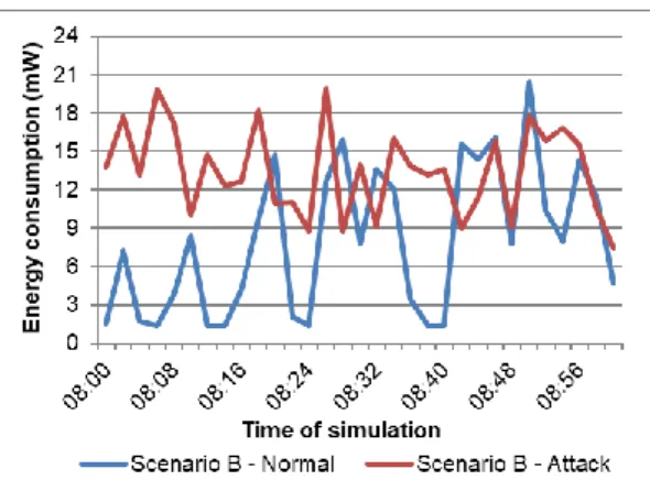
First of all, we show in Figure 2 the average energy consumption of scenarios A and B. We present the sample of one minute of simulation in the charts for easy visualization of data. Moreover, the presented data in the charts are related to node 6, which was attacked in the malicious attack simulation. In the charts, we presented the raw energy data of the node to faithfully show how energy consumption occurs in simulations.
Figure 3 the average detection cycles measured for each scenario. The charts on the left show the performed cycles without any attack; the charts on the right show the performed cycles in proposed attacks. We defined the “possible detection cycles” as the maximum number of cycles that could be performed in 10 minutes of simulation. As larger was N, the shorter was the total of possible detection cycles. For example, as the algorithm collects energy samples every two seconds when N=4 the minimum time to complete a detection cycle is 16 seconds because the algorithm takes 8 seconds to fill each sample vector (steps 2 and 3). Thus, the equation to calculate the total of possible cycles𝑀𝑐𝑦𝑐𝑙𝑒𝑠
is described in (9), where 𝑇𝑠𝑖𝑚𝑢𝑙𝑎𝑡𝑖𝑜𝑛 is the total time of simulation in seconds, 𝑇𝑖𝑛𝑡𝑒𝑟𝑣𝑎𝑙 is the time interval to collect energy sample, and 𝑇𝑝𝑟𝑜𝑐𝑒𝑠𝑠𝑖𝑛𝑔 is the time to compute the metric calculations. We observed in simulations that the average of 𝑇𝑝𝑟𝑜𝑐𝑒𝑠𝑠𝑖𝑛𝑔 was less than 0.01 seconds and had no impact in 𝑀𝑐𝑦𝑐𝑙𝑒𝑠, because the algorithm collection step always collects the energy consumption sample every
two seconds in a synchronized way, even whether the processing step delayed a few milliseconds. In other words, the algorithm corrects the wait time for the next collection cycle when necessary to reach exactly two seconds interval from the previous cycle. Moreover, we considered that a cycle is performed only when the node executes all algorithm steps. Otherwise, if the condition is true in step 4 of the algorithm, then the cycle is interrupted and not computed. Besides that, we show in
Figure 3 the performed cycles for each 𝜆 value simulated. The charts on the left show the performed cycles in scenarios without attack, while the charts on the right show the performed cycles with the proposed attacks.
𝑀𝑐𝑦𝑐𝑙𝑒𝑠 = 𝑇𝑠𝑖𝑚𝑢𝑙𝑎𝑡𝑖𝑜𝑛
𝑁 ∙ 𝑇𝑖𝑛𝑡𝑒𝑟𝑣𝑎𝑙 ∙ 2+ 𝑇𝑝𝑟𝑜𝑐𝑒𝑠𝑠𝑖𝑛𝑔 (9)
Thirdly, Table 2 shows the F1 scores obtained in scenario A for Sibson, Euclidian, and
Hellinger distances, respectively. In the same way, Table 3 shows the F1 scores obtained in scenario
B. The rows represent the simulations performed with different values of N and 𝜆. The columns represent the values of δ that determine whether the computed distance metric is anomalous. As better is the F1 score, the darker is the background color of the cell. We omitted the Recall and Precision values to avoid excessive information. However, we select and discuss some of them related to the best F1 scores
FIGURE 2: AVERAGE ENERGY CONSUMPTION OF SENSORS.
Table 2
F1 score of Sibson Euclidian, and Hellinger distances in scenario A N Λ
Δ
SIBSON EUCLIDIAN HELLINGER
0.01 0.05 0.1 0.15 0.2 0.25 0.3 0.35 0.01 0.05 0.1 0.15 0.2 0.25 0.3 0.35 0.01 0.05 0.1 0.15 0.2 0.25 0.3 0.35 4 3 0.896 0.959 0.911 0.841 0.796 0.763 0.763 0.763 0.862 0.930 0.959 0.909 0.867 0.813 0.787 0.763 0.577 0.767 0.896 0.930 0.944 0.933 0.911 0.881 4 4 0.825 0.944 0.949 0.914 0.851 0.841 0.841 0.841 0.767 0.912 0.944 0.973 0.925 0.892 0.841 0.841 0.520 0.679 0.844 0.896 0.930 0.959 0.960 0.925 4 5 0.712 0.866 0.907 0.886 0.843 0.843 0.843 0.843 0.643 0.794 0.882 0.904 0.897 0.843 0.843 0.843 0.426 0.549 0.712 0.794 0.848 0.899 0.907 0.897 4 6 0.549 0.781 0.892 0.861 0.861 0.861 0.861 0.861 0.458 0.690 0.781 0.861 0.872 0.861 0.861 0.861 0.279 0.458 0.549 0.690 0.754 0.818 0.877 0.883 4 7 0.577 0.733 0.812 0.817 0.817 0.817 0.817 0.817 0.520 0.679 0.754 0.812 0.817 0.817 0.817 0.817 0.238 0.458 0.577 0.679 0.712 0.794 0.824 0.817 4 8 0.356 0.593 0.719 0.738 0.738 0.738 0.738 0.738 0.318 0.449 0.607 0.730 0.738 0.738 0.738 0.738 0.053 0.279 0.356 0.426 0.566 0.655 0.710 0.719 5 3 0.741 0.818 0.773 0.753 0.753 0.753 0.753 0.753 0.769 0.821 0.831 0.789 0.784 0.753 0.753 0.753 0.410 0.667 0.764 0.800 0.818 0.789 0.784 0.763 5 4 0.596 0.800 0.824 0.812 0.800 0.800 0.800 0.800 0.476 0.764 0.793 0.839 0.812 0.800 0.800 0.800 0.278 0.476 0.583 0.741 0.780 0.825 0.818 0.812 5 5 0.545 0.786 0.831 0.848 0.836 0.836 0.836 0.836 0.476 0.680 0.807 0.820 0.848 0.836 0.836 0.836 0.235 0.439 0.578 0.706 0.764 0.814 0.813 0.848 5 6 0.439 0.625 0.839 0.875 0.875 0.875 0.875 0.875 0.410 0.545 0.653 0.814 0.875 0.875 0.875 0.875 0.182 0.368 0.476 0.545 0.625 0.692 0.839 0.875 5 7 0.368 0.625 0.786 0.833 0.833 0.852 0.852 0.852 0.378 0.545 0.625 0.764 0.814 0.852 0.852 0.852 0.000 0.229 0.359 0.512 0.625 0.653 0.764 0.828 5 8 0.324 0.609 0.706 0.778 0.778 0.778 0.778 0.778 0.286 0.488 0.638 0.706 0.778 0.778 0.778 0.778 0.065 0.235 0.368 0.488 0.578 0.638 0.706 0.755 6 3 0.750 0.913 0.939 0.906 0.857 0.787 0.738 0.706 0.684 0.889 0.913 0.939 0.885 0.857 0.800 0.727 0.387 0.571 0.750 0.889 0.913 0.958 0.939 0.941 6 4 0.611 0.864 0.917 0.941 0.889 0.857 0.800 0.787 0.485 0.810 0.889 0.936 0.960 0.923 0.842 0.787 0.276 0.485 0.611 0.780 0.837 0.913 0.936 0.939 6 5 0.529 0.780 0.939 0.941 0.906 0.873 0.842 0.828 0.485 0.649 0.837 0.958 0.960 0.906 0.857 0.828 0.148 0.485 0.529 0.649 0.780 0.864 0.936 0.960 6 6 0.276 0.529 0.818 0.880 0.846 0.852 0.836 0.836 0.214 0.387 0.529 0.818 0.880 0.852 0.836 0.836 0.077 0.214 0.276 0.387 0.485 0.611 0.818 0.870 6 7 0.276 0.571 0.791 0.809 0.824 0.824 0.824 0.824 0.214 0.438 0.595 0.773 0.792 0.824 0.824 0.824 0.077 0.214 0.276 0.387 0.529 0.667 0.791 0.800 6 8 0.148 0.471 0.650 0.698 0.711 0.739 0.739 0.739 0.148 0.387 0.514 0.634 0.682 0.739 0.739 0.739 0.000 0.077 0.148 0.333 0.424 0.556 0.615 0.667 7 3 0.833 0.950 0.955 0.894 0.840 0.778 0.737 0.712 0.800 0.923 0.950 0.930 0.913 0.857 0.792 0.750 0.444 0.600 0.833 0.923 0.950 0.952 0.955 0.913 7 4 0.688 0.865 0.952 0.933 0.875 0.808 0.778 0.764 0.600 0.800 0.895 0.923 0.952 0.894 0.824 0.778 0.174 0.444 0.688 0.765 0.833 0.895 0.927 0.930 7 5 0.552 0.727 0.900 0.930 0.889 0.875 0.857 0.857 0.444 0.645 0.800 0.927 0.930 0.913 0.875 0.840 0.174 0.320 0.552 0.645 0.727 0.865 0.900 0.930 7 6 0.320 0.600 0.778 0.857 0.864 0.870 0.851 0.851 0.174 0.552 0.600 0.778 0.878 0.870 0.851 0.851 0.000 0.174 0.320 0.500 0.600 0.600 0.778 0.821 7 7 0.385 0.552 0.743 0.829 0.837 0.864 0.864 0.864 0.385 0.444 0.552 0.722 0.810 0.864 0.864 0.864 0.091 0.320 0.385 0.444 0.500 0.625 0.686 0.789 7 8 0.250 0.645 0.743 0.789 0.769 0.800 0.829 0.829 0.250 0.385 0.645 0.722 0.769 0.800 0.829 0.829 0.000 0.174 0.320 0.444 0.645 0.667 0.743 0.757 8 3 0.839 0.971 0.973 0.947 0.857 0.800 0.766 0.735 0.800 0.941 0.971 0.944 0.947 0.900 0.837 0.766 0.500 0.667 0.839 0.941 0.941 0.971 0.973 0.947 8 4 0.560 0.909 0.973 0.947 0.900 0.837 0.800 0.766 0.560 0.800 0.941 0.971 0.973 0.923 0.837 0.766 0.105 0.500 0.560 0.714 0.909 0.941 1.000 0.973 8 5 0.560 0.759 0.882 0.973 0.923 0.878 0.857 0.837 0.500 0.667 0.800 0.909 0.973 0.923 0.857 0.837 0.000 0.435 0.560 0.667 0.714 0.839 0.909 0.944 8 6 0.435 0.615 0.774 0.857 0.865 0.850 0.850 0.850 0.286 0.560 0.615 0.774 0.857 0.872 0.850 0.829 0.000 0.200 0.435 0.560 0.615 0.667 0.774 0.848 8 7 0.364 0.500 0.643 0.788 0.811 0.842 0.872 0.872 0.200 0.435 0.435 0.643 0.800 0.842 0.872 0.872 0.000 0.200 0.364 0.364 0.435 0.480 0.643 0.733 8 8 0.286 0.435 0.643 0.788 0.800 0.800 0.800 0.800 0.200 0.364 0.500 0.643 0.824 0.800 0.800 0.800 0.000 0.105 0.286 0.364 0.435 0.500 0.643 0.710
Table 3
F1 score of Sibson Euclidian, and Hellinger distances in scenario B N Λ
Δ
SIBSON EUCLIDIAN HELLINGER
0.01 0.05 0.1 0.15 0.2 0.25 0.3 0.35 0.01 0.05 0.1 0.15 0.2 0.25 0.3 0.35 0.01 0.05 0.1 0.15 0.2 0.25 0.3 0.35 4 3 0,841 0,886 0,857 0,813 0,771 0,747 0,747 0,747 0,841 0,865 0,897 0,878 0,857 0,796 0,779 0,747 0,480 0,730 0,829 0,865 0,883 0,878 0,857 0,831 4 4 0,721 0,880 0,854 0,841 0,787 0,787 0,787 0,787 0,655 0,845 0,880 0,883 0,847 0,831 0,787 0,787 0,449 0,607 0,710 0,812 0,880 0,883 0,875 0,847 4 5 0,607 0,776 0,800 0,786 0,782 0,782 0,782 0,782 0,528 0,710 0,776 0,816 0,795 0,782 0,782 0,782 0,279 0,528 0,607 0,689 0,758 0,817 0,810 0,815 4 6 0,582 0,776 0,835 0,805 0,805 0,805 0,805 0,805 0,510 0,742 0,794 0,827 0,815 0,805 0,805 0,805 0,279 0,449 0,607 0,700 0,769 0,817 0,835 0,825 4 7 0,500 0,610 0,704 0,730 0,730 0,730 0,730 0,730 0,449 0,582 0,600 0,686 0,730 0,730 0,730 0,730 0,150 0,417 0,500 0,519 0,586 0,656 0,686 0,694 4 8 0,449 0,633 0,706 0,725 0,725 0,725 0,725 0,725 0,348 0,545 0,623 0,716 0,725 0,725 0,725 0,725 0,053 0,279 0,480 0,545 0,621 0,667 0,716 0,725 5 3 0,830 0,900 0,906 0,817 0,773 0,716 0,707 0,699 0,784 0,897 0,900 0,903 0,892 0,806 0,753 0,707 0,421 0,681 0,830 0,897 0,900 0,918 0,889 0,853 5 4 0,735 0,862 0,892 0,829 0,773 0,744 0,734 0,734 0,622 0,792 0,897 0,900 0,853 0,817 0,744 0,734 0,333 0,558 0,735 0,769 0,857 0,881 0,903 0,853 5 5 0,558 0,792 0,857 0,836 0,789 0,767 0,767 0,767 0,500 0,735 0,792 0,852 0,831 0,778 0,767 0,767 0,235 0,462 0,558 0,708 0,769 0,842 0,852 0,831 5 6 0,421 0,609 0,759 0,769 0,746 0,746 0,746 0,746 0,286 0,524 0,638 0,750 0,750 0,746 0,746 0,746 0,065 0,286 0,421 0,488 0,591 0,680 0,750 0,754 5 7 0,333 0,558 0,727 0,767 0,754 0,754 0,754 0,754 0,235 0,500 0,545 0,727 0,767 0,754 0,754 0,754 0,125 0,235 0,333 0,500 0,558 0,667 0,741 0,759 5 8 0,333 0,545 0,654 0,714 0,759 0,759 0,759 0,759 0,235 0,410 0,596 0,654 0,737 0,759 0,759 0,759 0,000 0,182 0,333 0,410 0,512 0,565 0,627 0,679 6 3 0,780 0,936 0,960 0,889 0,814 0,738 0,716 0,706 0,750 0,864 0,936 0,939 0,941 0,857 0,787 0,716 0,333 0,649 0,780 0,864 0,936 0,939 0,960 0,906 6 4 0,571 0,844 0,920 0,889 0,828 0,774 0,738 0,727 0,485 0,750 0,889 0,917 0,906 0,873 0,774 0,727 0,214 0,438 0,611 0,718 0,791 0,894 0,939 0,906 6 5 0,485 0,684 0,783 0,830 0,807 0,754 0,742 0,742 0,387 0,611 0,718 0,800 0,863 0,793 0,742 0,742 0,148 0,276 0,485 0,571 0,684 0,750 0,800 0,840 6 6 0,333 0,595 0,756 0,808 0,786 0,786 0,786 0,786 0,276 0,438 0,632 0,756 0,792 0,786 0,786 0,786 0,148 0,276 0,333 0,438 0,556 0,700 0,773 0,816 6 7 0,148 0,375 0,711 0,760 0,769 0,792 0,792 0,792 0,077 0,214 0,424 0,682 0,760 0,792 0,792 0,792 0,000 0,077 0,148 0,214 0,323 0,579 0,682 0,723 6 8 0,214 0,424 0,619 0,723 0,723 0,723 0,723 0,723 0,148 0,333 0,457 0,619 0,723 0,723 0,723 0,723 0,000 0,077 0,214 0,276 0,424 0,457 0,634 0,711 7 3 0,727 0,923 0,930 0,894 0,824 0,778 0,737 0,712 0,688 0,895 0,950 0,952 0,930 0,857 0,808 0,737 0,320 0,552 0,727 0,865 0,923 0,952 0,930 0,933 7 4 0,500 0,865 0,905 0,889 0,840 0,792 0,764 0,750 0,444 0,727 0,833 0,923 0,909 0,894 0,792 0,750 0,250 0,385 0,500 0,645 0,865 0,923 0,927 0,884 7 5 0,444 0,727 0,878 0,889 0,833 0,808 0,778 0,764 0,444 0,600 0,727 0,900 0,909 0,816 0,778 0,764 0,174 0,320 0,444 0,600 0,688 0,800 0,850 0,905 7 6 0,320 0,625 0,821 0,844 0,833 0,840 0,824 0,824 0,320 0,552 0,706 0,821 0,826 0,840 0,824 0,824 0,000 0,250 0,385 0,500 0,645 0,706 0,821 0,837 7 7 0,320 0,533 0,722 0,780 0,800 0,826 0,826 0,826 0,250 0,444 0,581 0,703 0,791 0,826 0,826 0,826 0,091 0,174 0,320 0,444 0,533 0,625 0,722 0,769 7 8 0,174 0,429 0,629 0,700 0,732 0,762 0,762 0,762 0,091 0,250 0,467 0,611 0,700 0,762 0,762 0,762 0,000 0,000 0,250 0,250 0,370 0,467 0,629 0,649 8 3 0,800 0,914 0,944 0,923 0,878 0,818 0,766 0,735 0,800 0,909 0,914 0,944 0,944 0,900 0,857 0,766 0,435 0,667 0,800 0,909 0,914 0,944 0,944 0,947 8 4 0,435 0,800 0,944 0,947 0,878 0,837 0,783 0,750 0,364 0,714 0,839 0,941 0,973 0,923 0,818 0,766 0,200 0,364 0,435 0,615 0,800 0,909 0,914 0,919 8 5 0,364 0,667 0,882 0,895 0,857 0,818 0,783 0,783 0,286 0,435 0,714 0,882 0,919 0,857 0,783 0,766 0,200 0,200 0,364 0,435 0,560 0,714 0,848 0,889 8 6 0,286 0,560 0,750 0,842 0,837 0,818 0,800 0,800 0,200 0,435 0,593 0,750 0,850 0,818 0,800 0,800 0,105 0,200 0,286 0,435 0,500 0,593 0,710 0,800 8 7 0,105 0,364 0,621 0,743 0,737 0,769 0,800 0,800 0,105 0,286 0,417 0,645 0,686 0,769 0,800 0,800 0,000 0,105 0,200 0,286 0,364 0,417 0,621 0,688 8 8 0,200 0,480 0,600 0,706 0,722 0,757 0,757 0,757 0,200 0,348 0,462 0,600 0,743 0,757 0,757 0,757 0,000 0,200 0,200 0,286 0,417 0,462 0,621 0,625
Lastly, Figure 4 shows the comparison among average energy consumption of sensors in scenarios A and B, for none and each one of distance metrics. We also compared the energy consumption without our proposed algorithm and for each one of the proposed distance metrics. The charts on the left show the consumption for simulations without attacks, while the charts on the right show the consumption for simulations with the attacks. We aimed to compare the performance of each distance metrics in terms of energy consumption. Thus, we performed a total of four simulation rounds, being one of them without any metrics and three other simulation rounds for each one of the distance metrics. In the simulation round without any metrics, we did not deploy the algorithm in nodes to measure their energy consumption. While in simulations with distance metrics, we disabled step 4 of our algorithm, to execute the maximum number of detection cycles in 10 minutes of simulation. We also used the window size N=4 for such simulation, because as smaller the N value, the bigger the number of cycles of detection. In summary, we simulated the worst case for scenarios A and B in the simulation rounds with intrusion detection.
Figure 4: Average energy consumption per second in sensors for scenarios A and B.
5 DISCUSSION
In this section, we discuss the results of the simulations presented in the previous subsection. We also take notes about the performance of our proposal.
First of all, we presented the average energy consumption among sensors in Figure 2. In scenario A, we observed that the energy consumption in normal simulation (without attack) was higher
while a task was executed, and it was lower during intervals among the tasks. Moreover, the energy consumption in attack simulation had a higher average energy consumption and the variations were higher than in normal simulation. Meanwhile, in scenario B we observed the same behavior, but higher energy consumption in attack simulation, where the range of energy consumption was a bit higher than half of the energy consumption range in normal simulation. Despite this, the energy consumption of the normal and attack simulations had similarities in both scenarios A and B, which shows how difficult it is to discriminate them by simple graph observation. Furthermore, we observed that the energy consumption of nodes in the normal simulation was different between scenarios. In other words, the nodes in scenario B wasted much more energy than in scenario A, explained by the characteristics of each type of task used in such scenarios. Thus, we verified that an IDS based on energy behavior must be adaptive to support any type of scenario; so, it can be considered efficient and reliable.
Secondly, we presented the performed cycles of detection in Figure 3. We observed that in normal simulations of both scenarios the performed cycles were smaller than in attack simulations. In other words, the detection cycle was not performed all the time when there were no attacks, saving the energy of sensors. In scenario A, the higher the λ value, the lower the number of performed cycles in normal simulation, while that in attack simulation, the number of performed cycles was near the total number of possible cycles. In other words, the detection cycles were performed almost all the time in attack simulation, as expected. In the same way, we observed the same behavior in scenario B, but the average performed cycles in the normal simulation were higher than in scenario A, for the same λ values. The growth of the cycles executed in the normal simulation of scenario B is explained by the characteristics of the scenario, in which the sensors have greater demand than in scenario A. Furthermore, in attack simulation, the cycles were performed almost all the time for 3 ≤λ ≤6 in both scenarios, especially when N≥7. When λ>6, the number of the cycles executed decreased a bit because even with the attack, sometimes the average energy consumption of sensors in the proposed scenarios was not too higher than the expected energy consumption represented by λ. Despite this, the detection cycles were performed significantly, mainly whether compared with the normal simulation. In summary, the charts showed that the mechanism that suppresses detection tasks when unnecessary was efficient and saved sensors’ energy and processing.
Thirdly, we presented the F1 scores in Table 2 for scenario A and in Table 3 for scenario B. The highest F1 scores occurred when 3 ≤λ ≤6 for any metrics, although the score's performance also depended on δ value. In scenario A, we observed that, in general, our proposal presented the lowest scores when N=5. Such results are explained by the characteristics of scenario A, where the sink requested sensing data from nodes every five seconds. In other words, such time interval was the same value of window size N. Thereby, the two slots A and B of the algorithm were fulfilled with similar
energy samples. For example, the first four positions of slots A and B were filled with energy samples from when the node was in standby mode, while the last position was filled with the energy sample from when the node was executing a task. Consequently, the false-positive rates were increased. Meanwhile, we observed in scenario B that the best F1 scores were measured when 3 ≤λ ≤5 for any metrics. Moreover, in general, as bigger the N value the better the F1 scores. Nevertheless, the main information that we observed in Tables 2 and 3 was that each one of the distance metrics had different performances for the same δ values. In other words, each one of the distance metrics presented the best F1 scores in different δ values.
In synthesis, we compiled the best F1 scores for all distance metrics in Table 4. We also present the recall and precision values in the same table, besides the best N, λ, and δ values used for each metric. We chose such values by comparing the performance in both scenarios. We care about finding the same N and λ values that performed the best possible F1 score for both scenarios. Thus, we added the F1 score from both scenarios (for the same N, λ, and δ values) divided by 2. Thereby, we observed that the best values of N and λ were 8 and 4, respectively. As cited before, we noted that the best δ value depends on the distance metric used in the detection task. Sibson metric had the lowest best δ value, while the Hellinger had the highest. Despite this difference, all metrics had similar performances. Only the Hellinger metric had a bit lower F1 score than other metrics in scenario B, explained by the Recall value. We highlight that the Recall values lower than one in Table 4 were caused by some few false-negatives events in attack simulation. Additionally, the Precision values lower than one in both scenarios were caused by some few false-positives events in the normal simulation.
Table 4
The best F1 scores for scenarios A and B
METRIC SCENARIO N Λ Δ F1
SCORE RECALL PRECISION
Sibson A 8 4 0,1 0,973 1,000 0,947 B 0,944 0,944 0,944 Euclidian A 8 4 0,2 0,973 1,000 0,947 B 0,973 1,000 0,947 Hellinger A 8 4 0,3 0,973 1,000 0,947 B 0,914 0,889 0,941
Lastly, we presented the energy consumption performance of the algorithm in Figure 4. We observed that the detection task increased a little bit the average energy consumption of a sensor for any scenario. Moreover, there were some differences in the range of energy consumption among metrics. We could not determine the worst metric in terms of energy consumption, because each metric presented different average values depending on scenario and simulation. Such differences can be
explained by several factors, but mainly because the sink and attacker requisition may change the order of processing and transmission of a task in a sensor. Despite this, such details are not relevant, because the difference in average energy consumption among metrics is very small. Moreover, if we get the worst average value, that was of the Hellinger metric in the (d), we will observe that such metric consumed only 4.34% more energy than the same simulation without our intrusion detection algorithm. In summary, all metrics consumed very small energy on task detection, demonstrating that the algorithm reached its goal of being lightweight and energy-efficient.
6 CONCLUSIONS AND FUTURE WORKS
In this work, we addressed the intrusion detection of energy-based attacks in IoT sensors. Our proposal implemented a standalone intrusion detection task in IoT sensors to detect those types of attacks. We proposed a lightweight statistical anomaly detection model that collects and analyses energy consumption data of sensors. Thus, we studied the deployment of Sibson, Euclidian, and Hellinger distance metrics on energy consumption data of IoT sensors to detect energy-based attacks. The goal was to evaluate the performance of those metrics in IoT scenarios, differentiating the energy consumption of a standard behavior from that one of an energy-based malicious attack. We simulated our proposed algorithm in two different scenarios, named A and B. We compiled the results and applied the F-measure approach to assessing the effectiveness of our model. The results showed an efficient algorithm to detect anomalies in energy consumption of nodes. The three metrics had similar performance on detection, although they worked better with different values of discrimination threshold δ.
Moreover, our approach showed that it is possible to perform an anomaly detection mechanism at sensors level without compromising the device resources. Additionally, our proposed algorithm avoids traffic exchange among sensors nodes and any other external device on intrusion detection task, showing an autonomous, lightweight, and energy-efficient solution. Such characteristics make our approach different from existing intrusion detection systems against energy-based IoT attacks.
Lastly but not least, we will address some improvements in future works. We observed in simulations that the λ parameter must be appropriately set to represent well the expected energy consumption of nodes. In other words, λ is one of the key parameters to adapt our algorithm for any scenario. Thus, we intend to develop a mechanism to set the best value of the λ parameter. Moreover, we intend to test our approach in silent energy-based attacks, that is, attacks that do not change the IoT network traffic. In addition, we would like to integrate our intrusion detection algorithm with existing countermeasures mechanisms, in order to mitigate the energy-based attacks.
REFERENCES
[1] A. J. F. N. Cavalcanti, F. P. Correia, and J. A. Brito, “Validation of a wireless sensor network applied to the irrigated fruitculture of the valley of São Francisco,” Brazilian Appl. Sci. Rev., vol. 4, no. 5, pp. 2763–2780, 2020.
[2] E. Manavalan and K. Jayakrishna, “A review of Internet of Things (IoT) embedded sustainable supply chain for industry 4.0 requirements,” Comput. Ind. Eng., vol. 127, pp. 925–953, Jan. 2019. [3] Y. P. Tsang, K. L. Choy, C. H. Wu, G. T. S. Ho, and H. Y. Lam, “An internet of things (IoT)-Based shelf life management system in perishable food e-commerce businesses,” in PICMET 2019 - Portland International Conference on Management of Engineering and Technology: Technology Management in the World of Intelligent Systems, Proceedings, 2019.
[4] Gartner, “Gartner Says Digital Transformation and IoT Will Drive Investment in IT Operations Management Tools Through 2020,” 2017. [Online]. Available: https://www.gartner.com/en/newsroom/press-releases/2017-07-26-garter-says-digital-transformation-and-iot-will-drive-investment-in-it-operations-management-tools-through-2020. [Accessed: 26-May-2019].
[5] J. Bradley, J. Barbier, and D. Handler, “Embracing the Internet of Everything To Capture Your Share of $14.4 Trillion,” White Paper, 2013. [Online]. Available: http://www.cisco.com/c/dam/en_us/about/ac79/docs/innov/IoE_Economy.pdf. [Accessed: 26-May-2019].
[6] Ericsson, “Internet of Things forecast – Ericsson Mobility Report,” 2016. [Online]. Available: https://www.ericsson.com/en/mobility-report/internet-of-things-forecast. [Accessed: 13-Jun-2019].
[7] W. Na, J. Park, C. Lee, K. Park, J. Kim, and S. Cho, “Energy-Efficient Mobile Charging for Wireless Power Transfer in Internet of Things Networks,” IEEE Internet Things J., vol. 5, no. 1, pp. 79–92, 2018.
[8] D. Zhai, R. Zhang, L. Cai, B. Li, and Y. Jiang, “Energy-Efficient User Scheduling and Power Allocation for NOMA based Wireless Networks with Massive IoT Devices,” IEEE Internet Things J., vol. 5, no. 3, pp. 1857–1868, 2018.
[9] A. Krishnakumar and V. Anuratha, “Survey on Energy Efficient Load-Balanced Clustering Algorithm based on Variable Convergence Time for Wireless Sensor Networks,” 2016.
[10] N. K. Pour, “Energy Efficiency in Wireless Sensor Networks,” 2016.
[11] T. Rault, A. Bouabdallah, and Y. Challal, “Energy efficiency in wireless sensor networks: A top-down survey,” Comput. Networks, vol. 67, pp. 104–122, 2014.
[12] T. Sanislav, S. Zeadally, G. D. Mois, and S. C. Folea, “Wireless energy harvesting: Empirical results and practical considerations for Internet of Things,” J. Netw. Comput. Appl., vol. 121, pp. 149– 158, Nov. 2018.
[13] D. E. Kouicem, A. Bouabdallah, and H. Lakhlef, “Internet of things security: A top-down survey,” Comput. Networks, Mar. 2018.
[14] K. Sha, W. Wei, T. Andrew Yang, Z. Wang, and W. Shi, “On security challenges and open issues in Internet of Things,” Futur. Gener. Comput. Syst., vol. 83, pp. 326–337, Jun. 2018.
[15] J. Lin, W. Yu, N. Zhang, X. Yang, H. Zhang, and W. Zhao, “A Survey on Internet of Things: Architecture, Enabling Technologies, Security and Privacy, and Applications,” IEEE Internet Things J., pp. 1–1, 2017.
[16] J. Grover and S. Sharma, “Security issues in Wireless Sensor Network - A review,” in 2016 5th International Conference on Reliability, Infocom Technologies and Optimization (Trends and Future Directions) (ICRITO), 2016, pp. 397–404.
[17] F. A. Alaba, M. Othman, I. A. T. Hashem, and F. Alotaibi, “Internet of Things security: A survey,” J. Netw. Comput. Appl., vol. 88, pp. 10–28, Jun. 2017.
[18] B. B. Zarpelão, R. S. Miani, C. T. Kawakani, and S. C. de Alvarenga, “A survey of intrusion detection in Internet of Things,” J. Netw. Comput. Appl., vol. 84, pp. 25–37, 2017.
[19] J. R. Patil and M. Sharma, “Survey of Prevention Techniques for Denial Service Attacks (DoS) in Wireless Sensor Network,” Int. J. Sci. Res. (IJSR), ISSN 2319-7064, vol. 5, no. 3, pp. 1065–1069, 2016.
[20] M. Dabbagh and A. Rayes, “Internet of Things Security and Privacy,” in Internet of Things From Hype to Reality, Cham: Springer International Publishing, 2019, pp. 211–238.
[21] O. A. Osanaiye, A. S. Alfa, and G. P. Hancke, “Denial of Service Defence for Resource Availability in Wireless Sensor Networks,” IEEE Access, vol. 6, pp. 6975–7004, 2018.
[22] N. Neshenko, E. Bou-harb, J. Crichigno, G. Kaddoum, and N. Ghani, “Demystifying IoT Security : An Exhaustive Survey on IoT Vulnerabilities and a First Empirical Look on Internet-scale IoT Exploitations,” IEEE Commun. Surv. Tutorials, vol. PP, no. c, pp. 1–30, 2019.
[23] Sheng Wei, Jong Hoon Ahnn, and Miodrag Potkonjak, “Energy Attacks and Defense Techniques for Wireless Systems,” in Proceedings of the sixth ACM conference on Security and privacy in wireless and mobile networks, 2013.
[24] T. Chen, H. Tang, X. Lin, K. Zhou, and X. Zhang, “Silent Battery Draining Attack against Android Systems by Subverting Doze Mode,” in 2016 IEEE Global Communications Conference (GLOBECOM), 2016, pp. 1–6.
[25] Contiki, “Contiki: The Open Source Operating System for the Internet of Things,” 2015. [Online]. Available: http://www.contiki-os.org/. [Accessed: 26-May-2019].
[26] Y. Sasaki, “The truth of the F-measure,” Teach Tutor mater, pp. 1–5, 2007.
[27] P. Pongle and G. Chavan, “A survey: Attacks on RPL and 6LoWPAN in IoT,” in 2015 International Conference on Pervasive Computing (ICPC), 2015, pp. 1–6.
[28] V. Desnitsky, I. Kotenko, and D. Zakoldaev, “Evaluation of Resource Exhaustion Attacks against Wireless Mobile Devices,” Electronics, vol. 8, no. 5, p. 500, May 2019.
[29] A. Merlo, M. Migliardi, and P. Fontanelli, “On energy-based profiling of malware in Android,” in 2014 International Conference on High Performance Computing & Simulation (HPCS), 2014, pp. 535–542.
[30] P. Pongle and G. Chavan, “Real Time Intrusion and Wormhole Attack Detection in Internet of Things,” Int. J. Comput. Appl., vol. 121, no. 9, pp. 975–8887, 2015.
[31] S. U. Jan, S. Ahmed, V. Shakhov, and I. Koo, “Toward a Lightweight Intrusion Detection System for the Internet of Things,” IEEE Access, vol. 7, pp. 42450–42471, 2019.
[32] C. Raju, “Defending Against Resource Depletion Attacks in Wireless Sensor Networks,” 2014. [33] C. T. Hsueh, C. Y. Wen, and Y. C. Ouyang, “A secure scheme against power exhausting attacks in hierarchical wireless sensor networks,” IEEE Sens. J., vol. 15, no. 6, pp. 3590–3602, 2015.
[34] T.-H. Lee, C.-H. Wen, L.-H. Chang, H.-S. Chiang, and M.-C. Hsieh, “A Lightweight Intrusion Detection Scheme Based on Energy Consumption Analysis in 6LowPAN,” Springer, Dordrecht, 2014, pp. 1205–1213.
[35] A. Azmoodeh, A. Dehghantanha, M. Conti, and K.-K. R. Choo, “Detecting crypto-ransomware in IoT networks based on energy consumption footprint,” J. Ambient Intell. Humaniz. Comput., pp. 1– 12, Aug. 2017.
[36] S. Yu, T. Thapngam, J. Liu, S. Wei, and W. Zhou, “Discriminating DDoS flows from flash crowds using information distance,” in NSS 2009 - Network and System Security, 2009, pp. 351–356. [37] Y. Tao and S. Yu, “DDoS Attack Detection at Local Area Networks Using Information Theoretical Metrics,” in 2013 12th IEEE International Conference on Trust, Security and Privacy in Computing and Communications, 2013, pp. 233–240.
[38] M. Xie, J. Hu, S. Guo, and A. Y. Zomaya, “Distributed Segment-Based Anomaly Detection with Kullback-Leibler Divergence in Wireless Sensor Networks,” IEEE Trans. Inf. Forensics Secur., vol. 12, no. 1, pp. 101–110, 2017.
[39] M. M. Deza and E. Deza, “Encyclopedia of Distances,” in Encyclopedia of Distances, Berlin, Heidelberg: Springer Berlin Heidelberg, 2009, pp. 1–583.
[40] Contiki, “SensorData.java - Contiki Source Code,” GitHub, 2008. [Online]. Available: https://github.com/contiki-os/contiki/blob/master/tools/collect-
view/src/org/contikios/contiki/collect/SensorData.java. [Accessed: 26-May-2019].
[41] A. Dunkels, F. Österlind, and Z. He, “An adaptive communication architecture for wireless sensor networks,” in Proceedings of the 5th international conference on Embedded networked sensor systems - SenSys ’07, 2007, p. 335.