ASSOCIAÇÃO DE POLITÉCNICOS DO NORTE (APNOR) INSTITUTO POLITÉCNICO DE BRAGANÇA

(1)

ASSOCIAÇÃO DE POLITÉCNICOS DO NORTE (APNOR)

INSTITUTO POLITÉCNICO DE BRAGANÇA

“A

n Analysis of Economic Convergence in EU from 2005 to 2016

”

Hanna Valentsinovich

Final Dissertation submitted to

Instituto Politécnico de Bragança

To obtain the Master Degree in Management, Specialisation in Business

Management

Supervisors:

António J.S.T. Duarte

Elena Petrushkevich

(2)

ASSOCIAÇÃO DE POLITÉCNICOS DO NORTE (APNOR)

INSTITUTO POLITÉCNICO DE BRAGANÇA

“

An Analysis of Economic Convergence in EU from 2005 to 2016

”

Hanna Valentsinovich

Supervisors:

António J.S.T. Duarte

Elena Petrushkevich

(3)

iii

Abstract

One of the main priorities of the European Union is promoting growth-enhancing conditions and reducing inequalities between levels of development among its Member States, which are key targets of the European Cohesion Policy. Since its inception, the objective of the policy was defined as the promotion of convergence between EU regions, in particular economic convergence, the reduction of regional disparities in the level of development that has been measured as convergence of GDP per capita relative to the EU average. This indicator has become one of the main ways in evaluating the European Сohesion Policy’s effectiveness.

The main purpose of this research is to assess if EU economies are converging. Therefore, the objectives of the research were: (1) to clarify the concepts of convergence: beta-convergence and sigma-convergence, (2) to review the different methods of convergence estimation and (3) to provide an update assessment of regional disparities in the European Union, using various estimation methods for the period from 2005 to 2016.

For the study, it was used secondary data for 276 NUTS 2 level regions from Eurostat.

The results of convergence estimation with help of Lorenz Curves, Gini coefficient and Robin Hood coefficient, kernel density estimation of the GDP per capita distribution and the cumulative frequency distribution curve showed existence of σ-convergence or reduction of disparities among regions in time. At the same time the results of increasing Variation coefficient detected divergence process.

The results of linear regression analysis, Salter graph and Markov analysis of transition probability matrix

indicated existence of β-convergence, defined as negative relationship between the initial income level

and subsequent income growth rate. It means that poorer regions of EU tend to catch up with the rich ones in terms of the level of income per capita.

(4)

iv

Resumo

Uma das principais prioridades da União Europeia é a promoção de condições favoráveis ao

crescimento e a redução das desigualdades entre os níveis de desenvolvimento dos seus Estados

Membros, que são dos principais alvos da política de coesão europeia. Desde a sua criação, o objetivo

da política foi definido como a promoção da convergência entre as regiões da UE, em particular, a

convergência económica, a redução das disparidades regionais no nível de desenvolvimento que foi

medido como a convergência do PIB per capita em relação à média da UE. Este indicador tornou-se

uma das principais formas de avaliar a eficácia da política europeia de coesão.

O objetivo principal desta pesquisa é verificar se as economias da UE estão a convergir. Portanto, os

objetivos da pesquisa foram: (1) esclarecer os conceitos de convergência: convergência beta e

convergência sigma, (2) rever os diferentes métodos de estimação da convergência e (3) proporcionar

uma avaliação atualizada das disparidades regionais na União Europeia, usando vários métodos de

estimação para o período de 2005 a 2016.

Para o estudo, foram utilizados dados secundários para 276 regiões do nível NUTS 2 do Eurostat.

Os resultados da estimação da convergência com auxílio das Curvas de Lorenz, Coeficiente de Gini e

Coeficiente de Robin Hood, estimativa da densidade da distribuição do PIB per capita e da curva de

distribuição de frequência acumulada, mostraram existência de convergência sigma ou redução de

disparidades entre regiões no tempo. Ao mesmo tempo, os resultados do aumento do coeficiente de

variação detetaram um processo de divergência.

Os resultados da análise de regressão linear, gráfico de Salter e da análise de Markov à matriz de

probabilidades de transição, indicaram a existência de convergência beta, definida como relação

negativa entre o nível de riqueza inicial e a taxa de crescimento da riqueza subsequente. Isso significa

que as regiões mais pobres da UE tendem a alcançar as mais ricas em termos do nível de rendimento

per capita.

(5)

v

Реферат

Одним из основных приоритетов Европейского союза является содействие улучшению условий роста и сокращению неравенства между уровнями развития среди его государств-членов. Эти

аспекты являются ключевыми задачами Европейской политики сплочения. С момента своего создания цель политикисплоченияопределялась как содействие конвергенции между регионами ЕС, в частности экономическойконвергенции, сокращение региональных диспропорций в уровне развития, которое выражается как конвергенция показателя ВВП на душу населения по сравнению со средним показателем по ЕС, Этот критерий стал одним из основных методов оценки эффективности политики сплочения в рамках ЕС.

Основная цель этого исследования - ответить на вопрос сближаются ли экономики стран ЕСв

своем экономическом развитии. Поэтому цели исследования заключаются в следующем: (1)

раскрыть понятие экономической конвергенции, а такжепояснить концепциибета-конвергенции

и сигма-конвергенции, (2) изучить методы оценки конвергенции, (3) предоставить актуальную

оценку регионального неравенствав Европейском союзе с использованием различных методовв период с 2005 по 2016 гг.

В ходе исследования использовались данные по 276 регионам 2 уровня Номенклатуры территориальных единиц для целей статистики статистической службы Европейского союза.

Результаты оценки конвергенции с использованием кривых Лоренца, коэффициента Джини и коэффициента Робина Гуда, оценки плотности ядра распределения ВВП на душу населения, кривой кумулятивного распределения частот показали наличие σ-конвергенции или уменьшение

различий между регионами во времени. В то же время результаты вычисленийкоэффициента вариации говорят o дивергенции регионов Европейского Союза.

При этом результаты линейного регрессионного анализа, построения графикаСолтера и анализ вероятностной матрицы цепного перехода Маркова свидетельствуют о β-конвергенции,

определяемой как отрицательная связь между начальным уровнем дохода и последующим уровнем ростадоходов. Это означает, что более бедные регионыЕС склонны догонять регионы с более богатые с точки зрения уровня дохода на душу населения.

(6)

vi

Abbreviations and/or Acronyms

EU - European Union

GDP - Gross domestic product KDE – Kernel Density Estimation

(7)

vii

List of Figures

Figure 1. Possible evolution of the GDP per capita of the poor countries (S) in relation to the rich ones

(B) in period T ... 4

Figure 2. Lorenz Curve. ... 6

Figure 3. Lorenz Curve graph with areas for Gini coefficient calculation……… ..7

Figure 4. Robin Hood Coefficient………...8

Figure 5. A sample histogram for a toy univariate dataset of seven data points...9

Figure 6. An example demonstrating the idea of the kernel density estimation with Gaussian kernels with different bandwidths...10

Figure 7. NUTS classification of regions………...14

Figure 8. NUTS 2 regions map ………..………...15

Figure 9. GDP per capita distribution for EU-28 in 2005 and 2016 ………...18

Figure 10. GDP per capita in % to EU-28 average distribution map in EU-28 by NUTS 2 in 2005 ... 19

Figure 11. GDP per capita in % to EU-28 average distribution map in EU-28 by NUTS 2 in 2016 ... 20

Figure 12. Plot estimation of growth equation for EU NUTS 2 from 2005 to 2016 ... 21

Figure 13. Variation Coefficient trend for EU-28 NUTS 2 level from 2005 to 2016. ... 22

Figure 14. Variation Coefficient trend for EU-17 NUTS 2 level from 2005 to 2016. ... 22

Figure 15. EU Lorenz Curves for 2005 and 2016. ... 23

Figure 16. EU Lorenz Curves Comparison for 2005 and 2016. ………...24

Figure 17. Gini index trend from 2005 to 2016. ... 25

Figure 18. Robin Hood index trend from 2005 to 2016. ... 25

Figure 19. KDE GDP per capita distribution for EU-28 in 2005 and 2016. ... 26

Figure 20. GDP per capita cumulative frequency distribution for EU-28 in 2005 and 2016 distribution for EU-28 in 2005 and 2016. ... 27

Figure 21. Salter Graph for EU-28 in 2005 and 2016. ... 27

(9)

ix

List of Tables

Table 1. Combinations of relations between β-convergence and σ-convergence.. ... 4

Table 2. Thresholds for the size of the NUTS regions………14

(10)

1

Introduction

Under conditions of the increasing globalization of the world economy, the socio-economic convergence of neighboring countries is essential. One of the main priorities of the European Union is promoting growth-enhancing conditions and reducing inequalities between levels of development among its Member States, which are key targets of the European Cohesion Policy. The essential argument for EU regional policy is that balanced regional development is a prerequisite for social cohesion and increased competitiveness in the countries and regions of the EU. Since its inception, the objective of the policy was defined as the promotion of convergence between EU regions, in particular, economic convergence, the reduction of regional disparities in the level of development that has been measured as convergence of GDP per capita relative to the EU average. This indicator has become one of the main ways in

evaluating the European Policy’s effectiveness. The research of income disparities and convergence in

EU countries and regions is aimed at further development of EU regional policies to bridge the development gaps.

The main purpose of this research is to assess if EU economies are converging. Therefore, the objectives of the research were: (1) to clarify the concepts of convergence: beta-convergence and sigma-convergence, (2) to review the different and methods of convergence estimation and (3) to provide update assessment of regional disparities in the European Union, using various estimation methods for the period from 2005 to 2016.

(11)

1

1. Literature Review

1.1. Definition of economic convergence

The term «convergence» first appeared in economic literature in the 1940s and 1950s and was borrowed from the theory of systems and the theory of convergence. Nowadays in foreign economic literature still there is no clearly defined notion of «convergence». The most common can be considered the definition, in which the words «convergence», «similarity» or «assimilation» are used during the analysis of the socio-economic space of countries. In the interdisciplinary approach to convergence, it can be identified with the similarity or also assimilation of countries in specific areas of existence of the individual and society (Lukianenko, Chuzhykov, Wozniak, 2013).

(12)

2

exchange rate system within at least two years. On the contrary measurement of real convergence is made with a use of chosen real macroeconomic aggregate. The aggregate most often used in empirical studies is GDP in real terms in conversion per capita or per worker (Dvorokova, 2013).

Real economic convergence in the broadest sense can be understood as a process of limiting economic inequalities between countries and regions. This interpretation of convergence is connected primarily with the question of the similarity of indices reflecting economic development, especially those that characterize the growth rate and GDP per capita; budget deficit; social spending; current revolving account; balance of foreign trade; the aggregate of other structural changes in the socio-economic domestic economy belonging to the technical infrastructure and environmental protection, industry, agriculture and service sector, labour market, technology market, market for the distribution of public subsidies and so on (Lukianenko, Chuzhykov, Wozniak, 2013).

In the narrow sense of the real convergence of the real sector there are several notions identified with convergence. It refers, first of all, to conditional and unconditional convergence, the convergence of

growth stages and income levels, β and σ-type convergence, global convergence and convergence

clubs. It should be emphasized that the clearest distinction is between conditional convergence and unconditional (absolute) convergence (Lukianenko, Chuzhykov, Wozniak, 2013).

In the absolute convergence hypothesis, the per capita incomes of countries or regions converge with one another in the long-term regardless of the initial conditions. Poorer countries and regions grow faster than richer ones and there is a negative relationship between average growth rates and initial income levels even if no other variables are included in the regression model as explanatory factors. It is assumed that all economies converge to the same unique and globally stable steady state equilibrium, which is a reasonable assumption in the case of a homogeneous sample of countries or regions (Paas, Kuusk, Schlitte, Võrk, 2007).

(13)

3

1.2. Beta-convergence and Sigma-convergence

In discussions of economic growth, two concepts of convergence appear. The first one took name of sigma-convergence (σ-convergence) refers to a reduction of disparities among regions in time (Monfort, 2008). It concerns cross-sectional dispersion, so in this context, convergence occurs if the dispersion of per capita income or product across a group of countries or regions declines over time. The σ -convergence enables it to be determined whether a variable is becoming increasingly more similar across the economies studied

.

The second concept was called as beta-convergence (β-convergence). It can be defined as a negative relationship between the initial income level and subsequent income growth rate. If poorer economies tend to catch up with the rich one in terms of the level of per capita income or product, there should also be a negative correlation between the initial income level and the growth rate (Paas, Kuusk, Schlitte, Võrk, 2007).

According to Iancu, (2007) the concept of β-convergence, generated by the analysis of the regression of

the development level of the countries/regions, may take three basic forms. Depending upon the depth of the analysis and the degree of compliance with the economic realities within the range allowed by the neoclassical model of convergent growth: (1) absolute β-convergence, (2) β-convergence clubs and (3)

conditional β-convergence.

These forms consist of the following:

1. The absolute β-convergence only takes into account the assumption of the high growth rates of the

poor countries as against the rich ones, irrespective of the differentiated evolution of the sample countries regarding the determinants of growth over the entire period of time (T) of the data used for the regression calculation.

2. The β-convergence clubs, which include the countries/regions that show some technological,

institutional and economic policy homogeneity, etc. The key assumption in case of convergence clubs requires that the same group should not show significant initial differences among the countries/regions of the club as regards the GDP. Despite the conceptual distinction, it is not easy to distinguish ‘club convergence’ from ‘conditional convergence’ empirically.

3.The conditional β-convergence hypothesis assumes that the negative correlation occurs only if some

(14)

4

Speaking about the relations between the two indicators, β-convergence and σ-convergence, during period T the following three combinations (C) may occur, which can be seen in the Table 1.

Table 1. Combinations of relations between β-convergence and σ-convergence.

C₁ C₂ C₃

𝜎𝑡𝑜+𝑇< 𝜎𝑡𝑜 (convergence)

𝜎𝑡𝑜+𝑇 > 𝜎𝑡𝑜 (divergence)

𝜎𝑡𝑜+𝑇>< 𝜎𝑡𝑜

(convergence, standstill, convergence)

-β (convergence) +β (divergence) ± β (divergence or convergence)

Decreasing distance between the development levels of the economies in

period T

Increasing distance between the development levels of the economies in

period T

Within period T, the decrease and increase in the distance between the development levels of the economies

may take place successively

Source: Iancu (2007, p.34).

The negative sign of the β parameter is the expression of the reverse relation between the annual average growth rate of the GDP per capita over the period T and the initial level of the GDP per capita in the year 𝑡₀(Iancu, 2007).

Figure 1 shows the third combination with fluctuations or even reversals of level of GDP per capita, that can happen in relation to the poor (S) and rich countries (B).

Figure 1. Possible evolution of the GDP per capita of the poor countries (S) in relation to the rich ones (B) in period T.

(15)

5

Sala-i-Martin X. and Barro R. (1990a), (1990b) draw attention that beta-convergence is a necessary but not sufficient condition for sigma-convergence to occur. A negative β-coefficient from a growth-initial level regression does not necessarily imply a reduction in variation of regional income or growth rates over time. This can be either because economies can converge towards one another, but random shocks push them apart or because, in the case of conditional Beta-convergence, economies can converge towards different steady-states (Monfort, 2008).

1.3. Estimation of convergence and convergence measures

In the literature, different methods of convergence estimation can be found.

Methodology to study β-convergence comes from original Baumol (1986) study of real convergence

between economies. Baumol has developed the so called conventional approach to convergence analysis. Through graphical projection of statistical data and through observed dependencies he has constructed an original growth Eq. 1:

1

T[ln(yi,T) − ln(yi,to)] = β1+ β2 ln(yi,to) + ɛt [1] where T is the end of time period, 𝒚_𝑻is real GDP per worker at the end of time period, 𝒕_𝒐 is the initial time period, 𝒚_𝒕_𝒐 is real GDP per worker at the beginning of time period, 𝜷_𝟏 is the intercept, 𝜷_𝟐 is the slope parameter, ε is statistical error term and iis index marking each country (Dvorokova, 2013). The measurement of sigma-convergence may be made by means of analytical tools and indicators. A frequently used indicator for the convergence measurement is the variation coefficient of the GDP per

capita denoted by σ and calculated as follows in the Eq.2:

𝜎𝑡= √_𝑛1∑ (𝑋𝑛_𝑖=1 𝑖𝑡− 𝑋̅𝑡)2∕ 𝑋̅𝑡 [2]

It may be used to characterize the convergence level by measuring the dispersion of the GDP per capita in a year, by means of the cross-section series (countries and regions). In this case, the relevance of the convergence indicator occurs only when comparisons are made. To characterize the convergence evolution (trend), time series (a discrete time interval, t and t+T) are used. When the phenomenon dispersion decreases over a period of time (when the indicator value diminishes over time), it means that convergence takes place, 𝜎_{𝑡𝑜+𝑇}< 𝜎_𝑡𝑜 (Iancu, 2007).

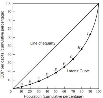
Another way to estimate convergence is to analyze changes in Lorenz Curve and Gini coefficient. Lorenz curve (first time developed by Max O. Lorenz in 1905) is a useful tool to analyse the inequality of wealth or income distribution, but it can also be used to study the concentration degree related to a certain development indicator in a group of countries, as in the European Union is (Albu, 2012).

(16)

6

within a certain population. Thus, on abscissa the cumulative share of people from lowest to highest GDP per inhabitant (X=Pc%) is marked and on the ordinate the corresponding cumulative share in GDP (Y=Yp%). The line passing through all points (x,y) in plane is the resulted Lorenz curve (Albu, 2012). The diagonal of the unit square thus formed means the average per capita level of GDP and the area delimited by the Lorenz curve and this diagonal, denoted by A, is considered to represent an aggregate measure of disparities or the degree of population concentration. The diagonal is corresponding to the so-called line of perfect GDP equality (all levels of GDP per capita are equal; by contrast, the line of perfect inequality is represented by the horizontal line, y=0 for all x less than 100%, continuing with the vertical line y=100% when x=100%) (Albu, 2012).

The example of the Lorenz Curve is shown on the Figure 2. It can be seen, that in the point F 60% of poorest population cover only 25% of the total GDP, and in the point G 90% of the population cover around 63% of total GDP.

Figure 2. Lorenz Curve. Source: Author's own elaboration.

(17)

7

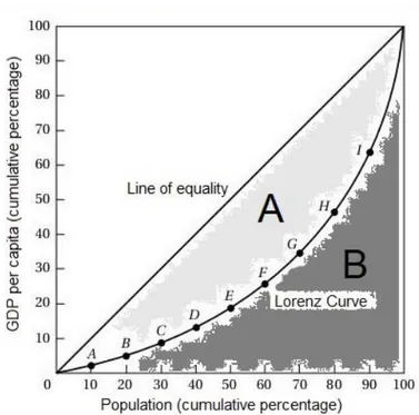
Figure 3. Lorenz Curve graph with areas for Gini coefficient calculation.

Source: Author's own elaboration.

So the relation for calculating the Gini coefficient (G) can be written, as follows in the Eq.3:

G = A / (A + B) [3] Theoretically, the Gini coefficient can range from 0 (perfect equality) to 1 (perfect inequality). Expressed as a percentage, the Gini coefficient is called the Gini index (Albu, 2012). A low value indicates more equal distribution (0 corresponding to perfect equality), while a high Gini coefficient indicates more unequal distribution (1 corresponding to perfect inequality where income is concentrated in the hands of one individual) (Monfort, 2008).

One of the methods used for estimating Gini coefficient on the basis of Lorenz Curve is interpolation, which produces less consistent results, but is less laborious. Thus, if the Lorenz curve is estimated for each interval as a line between two consecutive points, the area can be approximated by the so-called method of trapezoids. In this case, the relationship for calculating the Gini coefficient is as follows in the Eq.4:

G=1 –∑𝑛_𝑖=1(( 𝑋_𝑖− 𝑋_𝑖−1)/100%) ∗ ((𝑌_𝑖+ 𝑌_𝑖−1)/100%) [4]

(18)

8

Based on the Lorenz curve, another indicator that can be calculated by the Lorenz curve is the maximum vertical distance between the curve and the line of perfect equality (diagonal line), that is equal to OG section or 35% as shown on the Figure 4.

Figure 4. Robin Hood Coefficient.

It can be considered that the amount is equal to the proportion of total income that should be transferred from the richer half of the population to the poorest half of the population, given the idea to achieve equality in the distribution of income or GDP between entities (groups of persons, households, countries). Therefore, this indicator is sometimes called the Robin Hood coefficient or the RH index (when it is expressed as a percentage). For example, in the case of the distribution of the EU GDP expressed in PPS, the relationship for the RH index is as follows in the Eq. 5:

RH = max (Pc% - Yc%) [5] where: Pc% is the cumulative share of countries in the EU total population and Yc% is the cumulative share of countries in the EU total GDP (Albu, 2012).

(19)

9

A histogram is the simplest form of a nonparametric density estimation. The sample space is divided into disjoint categories, or bins and the density is approximated by counting how many data points fall into each bin. The histogram requires two parameters to be defined: the bin width h and the bin origin 𝒙_𝒐.

Figure 5. A sample histogram for a univariate dataset of seven data points.

Source: Gramacki (2018, p.8).

While the histogram is a very simple form of the nonparametric density estimator, there are some serious drawbacks that are already noticeable. First, the final shape of the density estimate strongly depends on the starting position of the first bin. Second, the natural feature of the histogram is the presence of discontinuities of density. These are not, however, related to the underlying density and, instead, are only an artifact of the chosen bin locations. The third drawback is the so-called curse of dimensionality, which constitutes a much more serious problem, since the number of bins grows exponentially with the number of dimensions. In higher dimensions one would require a very large number of examples or else most of the bins would be empty (incidentally, the curse of dimensionality phenomena is a common problem for all the nonparametric techniques for density estimation). All these drawbacks make the histogram unsuitable for most practical applications except for rapid visualization of results in one or two dimensions (Jenkins &Van Kerm, 2018).

One way to overcome these shortcomings is to use kernel density estimators. Under this method, each data point is the centre of normalised density function, referred to as the kernel. Densities are then added vertically to produce the estimation of the distribution. If a Normal is chosen as the density function, a Gaussian (stochastic) kernel density estimation of the distribution is obtained (Monfort, 2008).

(20)

10

small compared to the optimal value, producing the undersmoothed curve (it contains too many spurious bumps). In this example, the optimal bandwidth is about h = 0.8. In Figure 6c and 6d, the bandwidth is too big, producing the oversmoothed curves (it obscures much of the underlying structure of the input data).

Figure 6. An example demonstrating the idea of the kernel density estimation with Gaussian kernels

with different bandwidths. Source: Gramacki (2018, p.30).

A common way to determine the optimal bandwidth is to choose one that minimises an optimality criterion which is often selected as the Asymptotic Mean Integrated Squared Error (AMISE).

The techniques used in the context of kernel density estimation can be easily extended to consider various other probability distribution functions, as well as to the estimation of the cumulative distribution function of cumulative frequency distribution. The cumulative frequency is the percentage of observational units for which the record value falls below a reference value. In general, the steeper the curve representing the cumulative frequency around the mean, the less the distribution features large disparities.

(21)

11

on the horizontal axis and pointing out their level of GDP per capita on the vertical axis for a base year. Afterwards by holding the base year rank positions of regions constant on the horizontal axis, new series show the regions’ GDP per capita for subsequent years. As a result, any significant changes in the regional distribution of GDP per capita become visible. In addition, regions can be identified and their performance compared.

This method helps to reveal gradual change or persistence in the distribution of GDP per capita among the countries. Visually the processes of convergence can be seen as more horizontal series on the graph (Monfort, 2008).

For analysis of the distribution of EU regions’ GDP per capita it can be applied the methodology underlying Markov chain analysis. Markov chain analysis constitutes a powerful instrument capable of detecting individual movements within the distribution and of describing its dynamics.

First a set of nnon-overlapping regional GDP per head classes should be defined. Let 𝒅_𝒊𝒕 denote the percentage of regions in class i at time t. 𝒅_𝒕 = (𝒅_𝟏𝒕, …, 𝒅_𝒏𝒕) is the corresponding distribution over the selected classes. Afterwards another date is selected, denoted by t+1. Then it can be computed the proportion of regions from the category iin t and moving to category jin t+1. This information can be collected under the form of a transition probability matrix P, as for any two income classes iand j, the element Pijdefines the probability of moving from class ito j between time tand t+1.

For example, the value obtained for 𝑷_𝟏𝟐(the element of the first row, second column) means that this is a percentage of the regions which were in the first class in the moment t moved to second class in the moment t+1 (Monfort, 2008).

On the other hand, 𝑷_𝟏𝟏indicates the percentage of those countries that remained in the same class. The evolution of the distribution over time can be described by the following Eq. 6:

𝑑𝑡+1= P 𝑑𝑡 [6] If matrix P is assumed to be constant in time and the regions destributions 𝒅_𝒊𝒕 to be independent of its past values, then this equation can be analysed as a time homogeneous Markov chain, with properties of the transition probability matrix P conveying a series of information concerning the dynamics of the distribution. A Markov chain is ergodic if it is possible to go from every state (distribution) to any other state in a finite number of steps. Ergodicity and the existence of a stationary distribution is ensured when the modulus of the second eigenvalue of the transition matrix is strictly smaller than 1. Eigenvalues are defined as aa set of special scalars associated with a linear system of equations (that can always be written using a matrix). If the system of equations represents the evolution of an object (here a distribution) in time, eigenvalues convey information concerning its dynamics (e.g. existence of a

(22)

12

First, if Pis the transition probability matrix of an ergodic Markov chain, then the chain is characterised by a stationary distribution corresponding to a steady-state towards which the distribution will converge in time. This stationary distribution, which is sometimes referred to as the ergodic distribution, is an interesting element since it can be interpreted as a projection of the distribution in the future given the transition process described by P.

Second, it can be derived an indicator of the speed at which the distribution is supposed to converge to this steady-state. This can for instance be expressed as the half-life of the chain, i.e. the amount of time it will take to cover half the distance separating the current distribution from the stationary distribution. The half-life is defined as in the Eq. 7:

𝐻𝐿 = −𝑙𝑜𝑔 (2)/𝑙𝑜𝑔 (|𝜆2|) [7] where 𝝀_𝟐is the second eigenvalue of matrix P. A low value of the half-life indicates a rapid convergence to the steady-state (Chennubhotla, Jepson, 2002).

The matrix also provides information on the stability of the process, i.e. the probability of remaining in the same class. So, it can be calculated stability index for the transition matrix Pof dimension nas in the Eq. 8:

(23)

13

2. Research Methodology

2.1. Objective of the study and Research Hypotheses

The main objective of this research is to answer the question if EU are economies converging or not. To achieve this goal, it should be provided update assessment of regional disparities in the European Union on the basis of methods for economic convergence estimation, described in the chapter 1.

2.2. Description of Data Collection

For this study the secondary data from Eurostat databases have been used.Eurostat is the statistical office of the European Union situated in Luxembourg. Its main responsibilities are to provide statistical information to the institutions of the European Union and to promote the harmonisation of statistical methods across its member states (Eurostat, 2018a). The databases of Eurostat include levels of GDP per capita in % to EU-28 average and population of all countries and regions of EU for the period from 2005 to 2016. Data collection was carried out in March and April, 2018.

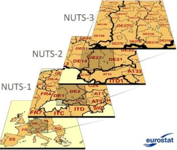
Comparing regional data that are as detailed as possible is often more meaningful and this also highlights the disparities — or similarities — within EU Member States themselves. So data for regions of NUTS 2 level was collected as well. The NUTS (Nomenclature of territorial units for statistics) classification — the classification of territorial units for statistics. This is a regional classification for the EU Member States providing a harmonised hierarchy of regions: the NUTS classification subdivides each Member State into regions at three different levels, covering NUTS 1, 2 and 3 from larger to smaller areas (Eurostat, 2018d). The current NUTS 2016 classification is valid from 1 January 2018 and lists 104 regions at NUTS 1, 281 regions at NUTS 2 and 1348 regions at NUTS 3 level.

(24)

14

• The collection, development and harmonisation of European regional statistics

• Socio-economic analyses of the regions o NUTS 1: major socio-economic regions

o NUTS 2: basic regions for the application of regional policies o NUTS 3: small regions for specific diagnoses

• Framing of EU regional policies.

o_{Regions eligible for support from cohesion policy have been defined at NUTS 2 level.} o_{The Cohesion report has so far mainly been prepared at NUTS 2 level.}

The NUTS regulation defines minimum and maximum thresholds for the size of the NUTS regions: Table 2. Thresholds for population for the size of the NUTS regions.

Level Minimum population Maximum population

NUTS 1 3 000 000 7 000 000

NUTS 2 800 000 3 000 000

NUTS 3 150 000 800 000

Source: Eurostat (2018g).

Despite the aim of ensuring that regions of comparable size all appear at the same NUTS level, each level still contains regions which differ greatly in terms of population (Eurostat, 2018g).

Figure 7. NUTS classification.

Source: Eurostat (2018d).

(25)

15

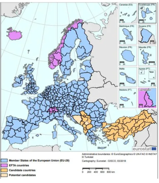
Figure 8. NUTS 2 regions map.

Source: Eurostat (2018f).

All the analysis performed in the research is based on data of Gross Domestic Product per capita. Gross domestic product (GDP) is a measure for the economic activity. It is defined as the value of all goods and services produced less the value of any goods or services used in their creation. The volume index of GDP per capita in Purchasing Power Standards (PPS) is expressed in relation to the European Union (EU-28) average set to equal 100. If the index of a country is higher than 100, this country's level of GDP per capita is higher than the EU average and vice versa. Basic figures are expressed in PPS, i.e. a common currency that eliminates the differences in price levels between countries allowing meaningful volume comparisons of GDP between countries (Eurostat, 2018b).

(26)

16

Finland, France, Germany, Greece, Hungary, Ireland, Italy, Latvia, Lithuania, Luxembourg, Malta, Netherlands, Poland, Portugal, Romania, Slovakia, Slovenia, Spain, Sweden, United Kingdom.

2.3. Description of Data Analysis

(27)

17

3. Presentation and Results Analysis

3.1. Initial descriptive analysis

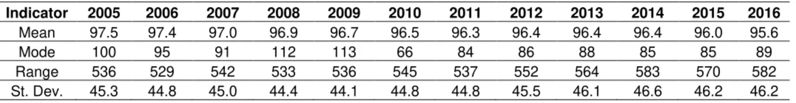
For the data set used in the research there were calculated some indicators that are presented in the table N. It can be concluded that the average value of GDP per capita in % by average EU decreased from 97.5 in 2005 to 95.6 in 2016. The region with lowest value has Bulgarian Severozapaden with 29 and the highest has Inner London -West. The difference between regions with minimum and maximum GDP per capita increased during last years and reached 582 in 2016. The deviation of values from the average lies within interval of 44.1-46.2.

Table 3. Values of indicators for description analysis for 2005-2016.

Indicator 2005 2006 2007 2008 2009 2010 2011 2012 2013 2014 2015 2016

Mean 97.5 97.4 97.0 96.9 96.7 96.5 96.3 96.4 96.4 96.4 96.0 95.6

Mode 100 95 91 112 113 66 84 86 88 85 85 89

Range 536 529 542 533 536 545 537 552 564 583 570 582

St. Dev. 45.3 44.8 45.0 44.4 44.1 44.8 44.8 45.5 46.1 46.6 46.2 46.2 Source: Author's own calculation based on Eurostat data.

(28)

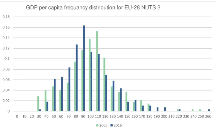
18

Figure 9. GDP per capita in % to EU-28 average distribution for EU-28 in 2005 and 2016.

Source: Author's own calculation based on Eurostat data.

In the Figure 10 is presented the map of GDP per capita in PPS in % to EU-28 average distribution by NUTS 2 in 2005. It can be seen, that out of 72 regions with lower GDP per capita the majority of them belongs to Bulgaria, Romania, Poland, Baltic countries (Lithuania, Latvia and Estonia), Czech Republic, Hungary, Slovakia, Croatia or in other words new Member States of EU. There are 83 regions with GDP per capita lower from EU average not more than 25 % (from 75 to 100) which are concentrated mostly in the west of Iberian Peninsula (Portugal and Western Spain), France and Eastern Germany. In the interval from 250 to 559 was observed only one region that is Inner London- West.

0 0.02 0.04 0.06 0.08 0.1 0.12 0.14 0.16 0.18

0 10 20 30 40 50 60 70 80 90 100 110 120 130 140 150 160 170 180 190 200 210 220 230 240 250 260

GDP per capita frequancy distribution for EU-28 NUTS 2

(29)

19

Figure 10. GDP per capita in % to EU-28 average distribution map in EU-28 by NUTS 2 in 2005.

Source: Eurostat (2018h).

(30)

20

same the classes with GDP per capita equal or slightly higher than EU average dropped from 103 to 82. The rest of the classes stayed almost the same.

Figure 11. GDP per capita in % to EU-28 average distribution map in EU-28 by NUTS 2 in 2016.

(31)

21

3.2. Analysis of results

The analysis of β-convergence was performed as described in the chapter 1.3 by estimating the growth equation 1 from which 𝛃_𝟐means the slope of the trend of difference of natural logarithms GDP per capita distribution curve from 2005 to 2016 and defines existence of β-convergence. Indeed, it can be seen that the regions with lower initial GDP per capita level reached in general grew more than other regions. The negative slope of the curve in Figure 12 with 𝛃_𝟐equal to -0.0046 shows that the speed of convergence is very low.

Figure 12. Plot estimation of growth equation for EU NUTS 2 from 2005 to 2016.

Next it will be presented the results of σ-convergence estimation performed with different methods. The

first method was analysis the variation coefficient. The following Table 4 shows the evolution of the coefficient of variation calculated for the EU-28 NUTS 2 regions for the period 2005-2016.

Table 4. Variation coefficients EU-28 NUTS 2 from 2005 to 2016.

Year Variation coefficient

2005 0.464

2006 0.459

2007 0.463

2008 0.457

2009 0.455

2010 0.463

2011 0.465

2012 0.471

2013 0.477

2014 0.483

2015 0.480

2016 0.482

y = -0.0046x + 0.064

-0.03 -0.02 -0.01 0 0.01 0.02 0.03 0.04 0.05 0.06 0.07

8 8.5 9 9.5 10 10.5 11 11.5 12 12.5

(32)

22

Figure 13. Variation Coefficient trend for EU-28 NUTS 2 level from 2005 to 2016.

The results show a downward trend from 2005 to 2009 and clear upward trend in 2009-2014 with variation coefficient increasing from 0.455 to 0.483. That means that from 2009 the Member States are diverging.

The variation coefficient trend for EU-17 NUTS 2 level (where EU-17 are new Member States, that entered EU after 2004) is presented in the Figure 14.

Figure 14. Variation Coefficient trend for EU-17 NUTS 2 level from 2005 to 2016.

Source: Author's own calculation based on Eurostat data. 0.450

0.455 0.460 0.465 0.470 0.475 0.480 0.485

2005 2006 2007 2008 2009 2010 2011 2012 2013 2014 2015 2016

0.340 0.360 0.380 0.400 0.420 0.440 0.460

(33)

23

The evolution of disparities among EU-17 regions shows a clear upward trend, the coefficient of variation increasing from 0.389 to 0.453, that means that even income distribution of states that entered EU more than 20 years ago are characterized by divergent processes.

Another method used in the research to analyse the reductions of disparities of income distribution Lorenz Curves were used by calculating the cumulated weights of GDP per capita and those of the population as percentages and building a graph. The results are presented as the Lorenz curve for the EU in 2005 and in 2016 in the Figures 15.

Figure 15. EU Lorenz Curves for 2005 and 2016.

For example, the Lorenz curve for the distribution of the EU GDP in 2016 shows that 75% of the EU population (the poorest 21 countries with a GDP per capita Index less than 118) covered only 61.66% of the total EU GDP and that 91% of the EU population covered only 66% of the total EU GDP. As for 2005, the Lorenz curve shows that 14% of the EU population (the poorest 4 countries with a GDP per capita Index less than 50) covered only 6.4% of the total EU GDP and that 89% of the EU population covered only 61.8% of the total EU GDP.

The comparison of the curves is shown in the Figure 16. 0% 10% 20% 30% 40% 50% 60% 70% 80% 90% 100% 0

7% _14% _21% _29% _36% _43% _50% _57% _64% _71% _79% _86% _93%

100%

EU Lorenz Curve in 2005

Lorenz Curve Diagonal

0% 10% 20% 30% 40% 50% 60% 70% 80% 90% 100% 0 7%

14% 21% 29% 36% 43% 50% 57% 64% 71% 79% 86% 93%

100%

EU Lorenz Curve in 2016

(34)

24

Figure 16. EU Lorenz Curve Comparison for 2005 and 2016.

It can be seen a diminution of the area bounded by the Lorenz curve and the diagonal in 2016 compared to 2005, which signifies a process of σ-convergence in this period.

According to the result of the calculation of Gini Index and Robin Hood Index, presented in the Table 5, there is a clear trend of σ-convergence during the period from 2006 to 2014 (as shown on the Figure 17), as the Gini coefficient estimated by the method of interpolation almost continuously decreased (from 15.76% to 12.2%), with exception of 2006, when Gini Index accounted for more than 25% of because of the shares of Spain, Italy, Cyprus I and Germany in total GDP of EU. The minimum value of the coefficient was reached in 2014 (10.15%), when in 2015 and 2016 there were somewhat higher values (12.84% and 11.12%, respectively).

Table 5. Gini Index and Robin Hood Coefficient for EU from 2005-2016. Year Gini Index Robin Hood Index

2005 15.76% 27.30%

2006 25.06% 29.84%

2007 15.76% 27.30%

2008 15.15% 28.17%

2009 12.59% 26.20%

2010 11.58% 24.16%

2011 12.48% 24.31%

2012 11.39% 24.29%

2013 11.05% 24.27%

2014 10.15% 21.75%

2015 12.84% 25.31%

2016 11.12% 25.11%

0% 10% 20% 30% 40% 50% 60% 70% 80% 90% 100% 0 4% 7%

11% 14% 18% 21% 25% 29% 32% 36% 39% 43% 46% 50% 54% 57% 61% 64% 68% 71% 75% 79% 82% 86% 89% 93% 96%

100%

(35)

25

Figure 17. Gini index trend from 2005 to 2016.

As for Robin Hood Index, it can be concluded that from 2006 till 2014 this indicator was gradually declining from 29.84% in 2006 to 21.31% in 2014, when in 2015 and 2016 the values rose to the level of 25%. That means, for example in 2016, that around 25% of total GDP should be transferred from the richer half of the EU population to the poorer half of the EU population in order to achieve equality in GDP distribution between EU members.

Figure 18. Robin Hood index trend from 2005 to 2016.

Source: Author's own calculation based on Eurostat data. 5.00%

10.00% 15.00% 20.00% 25.00% 30.00%

2005 2006 2007 2008 2009 2010 2011 2012 2013 2014 2015 2016

20.00% 22.00% 24.00% 26.00% 28.00% 30.00% 32.00%

(36)

26

The Gaussian kernel estimation of the GDP per capita distributions for the EU-28 for the years 2005 and 2016 is displayed in the following Figure 19.

Figure 19. KDE GDP per capita capita in % of the EU-28 average distribution for NUTS 2 in 2005 and

2016.

The evolution of the distributions between 2005 and 2016 indicates a convergence process at work for the EU-28. Frequencies around the values 110% of EU average in 2005 and 85% in 2016 significantly increase, while they tend to decrease for values below 60% and above 110% of the EU average in 2005 and below 85% and 120% in 2016. In addition, for the EU-28, the estimation reveals an evolution from a bimodal to a unimodal distribution. This is particularly interesting as most analysis had indeed detected a bimodal distribution from the 1980s through to the end of the 1990s, leading to the conclusion that a polarisation process was taking place in Europe, with a “club” of poor regions converging towards a low steady-state (around 40% of the EU average in 2005) and another club of richer regions converging towards a high steady-state (around 110% of the EU average in 2005).

The shape of the distribution in 2016 no longer shows signs of polarisation, making the scenario of various convergence clubs among EU regions less likely.

(37)

27

interval from 60% to 100% of EU GDP average, which confirms that convergence has taken place among EU regions between these two dates.

Figure 20. GDP per capita cumulative frequency distribution for EU-28 in 2005 and 2016.

The following Figure 21 shows the Salter graph for the EU-28, comparing the distributions of members GDP per capita in 2005 and 2016.

Figure 21. Salter Graph for EU-28 in 2005 and 2016.

Source: Author's own calculation based on Eurostat data. 0

0.1 0.2 0.3 0.4 0.5 0.6 0.7 0.8 0.9 1

0 10 20 30 40 50 60 70 80 90 100 110 120 130 140 150 160 170 180 190 200 210 220 230 240 250

2005 2016

30 80 130 180 230

G

DP PER CA

PIT

A

(38)

28

An initial observation is the general tendency for the horizontality of the series to increase between 2005 and 2016, reflecting a general decrease in the extent of regional disparities. It can be clearly seen the increase of in GDP per capita for new members states (poor regions catch up with the rich regions) – convergence process. The frequency of upward movements in the distribution is indeed higher in the low end of the distribution compared to that of downward movements in the high end of the distribution. Nevertheless, some countries, where relative GDP per capita is lower than average in EU, can be characterised with a decrease of the indicator during the period such as Portugal falling from 82 to 77 and Greece falling from 93 to 68. At the same time the richest countries stay at least at the same level in 2016 keep their relative GDP per capita growing from 147 to 183 for Ireland and from 247 to 258 for Luxembourg.

This information is conveniently complemented by mapping changes in GDP per head between 2005 and 2016.

Figure 32. Change in GDP per capita in % of the EU-28 average, 2005-2016.

(39)

29

The results of the Markov chain analysis are presented in the Table 6.

Table 6. Transition probability matrix for EU-28 NUTS 2 from 2005 to 2016.

Transition probability matrix

2016

2005

Percentage of

regions GDP per capita 0-50 51-75 76-100 101-150 151-

12% 0-50 0.59375 0.40625 0.00000 0.00000 0.00000

14% 51-75 0.10200 0.74359 0.15385 0.00000 0.00000

30% 76-100 0.00000 0.22892 0.71084 0.06024 0.00000

37% 101-150 0.00000 0.00971 0.24272 0.71845 0.02913

7% 151- 0.00000 0.00000 0.00000 0.15789 0.84211

Summary statistics

0-50 51-75 76-100 101-150 151-

Stationary distribution 12% 48% 32% 8% 1%

Half-life 5.1 periods

S 0.72

C101-150 0.25

C76-100 0.32

Source: Author's own elaboration based on Eurostat data.

The transition probability matrix indicates a relative persistence of the distribution. The values on the diagonal are quite high, especially in the class [151- ], suggesting a high probability of remaining in the same class of GDP per capita. This is also proved by stability index S which takes the value of 0.72. However, quite high percentage of the regions from class [0-50]- (40 %) managed to move in 2016 to the upper class. For other classes the movement to the upper class was not more than 15% of regions, while it was also observed the movement to lower classes. In particular, 24.3% of the regions from class [101-150] in 2005 moved one class down and almost 1% of the regions moved 2 classes down in 2016. In general, for regions with GDP per capita lower than 75% of the EU average, movements towards upper classes are much more frequent than movements down, the reverse being true for regions with GDP per capita above this threshold.

This shows a convergence process where poorer regions catch up on the richer ones. The frequencies of the distribution at the tails are lower, as clearly indicated by the stationary distribution. The distribution is therefore likely to feature fewer disparities in the long-run with a concentration of observations in the central categories. This is confirmed by the convergence index, measuring the probability of staying or moving to a cell (0.32 for convergence towards the class [101-150]; 0.25 for convergence towards the class [76-100]).

(40)

30

Table 7. Mean first passage time matrix for EU-28 NUTS 2 from 2005 to 2016.

Mean first passage time

0-50 51-75 76-100 101-150 151-

0-50 8.3734 2.4631 10.5879 58.2646 511.4903 51-75 18.161 2.1036 8.1249 55.8016 509.0273 76-100 23.6961 5.5352 3.1605 47.6767 500.9024 101-150 28.1554 9.9944 4.9992 13.327 453.2253 151- 34.4845 16.3236 11.3283 6.3291 72.609

Source: Author's own elaboration based on Eurostat data.

(41)

31

Conclusions, Limitations and Future Research Lines

The main objective of the research was analysing if EU Member States were converging in a 12 years period from 2005 to 2016.

In order to provide a theoretical framework for the issue in question, a literature review on the topic of economic convergence was provided along with the clarification of different types of convergence including absolute, conditional and club convergence, β-convergence and σ-convergence. As well, a wide range of different methods of convergence estimation were described. Understanding the theoretical background of the topic may be helpful for policy makers, especially in case of European Cohesion Policy, for effective implementing of measures.

To reach the proposed objective, convergence was estimated on the basis of information about GDP per capita in PPS in to EU-28 average distribution by NUTS 2 regions for the period from 2005 to 2016, collected from Eurostat databases for regional statistics. The analysis was performed using the following methods of convergence estimation: variation coefficient, Lorenz Curve, Gini coefficient and Robin Hood coefficient, analysis of frequency distribution and cumulative frequency distribution, kernel density estimation, Salter graphs, Markov analysis of transition probability matrices.

The results of convergence estimation with the following methods showed existence of σ-convergence or reduction of disparities among regions in time. Lorenz Curves indicated diminution of the area bounded by the Lorenz curve and the diagonal in 2016 compared to 2005. It was observed a continuous decrease of Gini coefficient and Robin Hood coefficient from 2006 to 2014. Kernel estimation of the GDP per capita distributions reveals an evolution from a bimodal to a unimodal distribution. A steeper character of the cumulative frequency distribution curve for 2016 in comparison to one of 2005 represents less disparities across EU-28 NUTS 2 regions. At the same time, the results of increasing variation coefficient detected a divergence process.

(42)

32

of transition probability matrix detects that for regions with GDP per capita lower than of the EU average, movements towards upper classes are much more frequent than movements down.

These results underline that the analysis of convergence is in fact very complex process. Serious assessments of convergence cannot be based on a single measure but rather on a panel of instruments and a sound interpretation of their results.

There were also some limitations to the present work. First, it should be noted that the result of the calculations may be not as accurate, as the analysed data was collected in relative value that probably was previously rounded off. Second, the current NUTS 2016 includes 281 regions at NUTS 2 level is valid only from 1 January 2018. At the same time all the calculations were performed with the data base of 276 regions, because the databases on Eurostat at the moment of collecting data were still organized according to the previous classification valid before 1 January 2018. Third, there is no convergence estimation method capable of capturing all relevant aspects of a convergence.

(43)

33

References

Albu, L. L. (2012) The convergence process in the EU estimated by Gini Coefficient. Romanian Journal of Economic Forecasting,4, 5-16.

Barro, R. & Sala-i-Martin X. (1990a) Convergence across States and Regions. Brookings Papers on Economic Activity,107-182.

Barro, R. & Sala-i-Martin X. (1990b) Economic growth and Convergence across the United States. NBER working paper series,1- 61.

Barro, R. (1991). Economic Growth in a Cross Section of Countries. The Quarterly Journal of Economics, Vol. 106, No. 2, 407-443.

Barro, R. & Sala-i-Martin, X. (1991). Convergence across States and Regions. Brookings Papers on Economic Activity, Vol. 22, No 1, 107-182.

Barro, R. & Sala-i-Martin, X., (1992). Convergence. [Online]. Available: http://www.nber.org/papers/w3419.pdf, Access Date: 02.02.2018.

Baumol, W. J. (1986) Productivity Growth, Convergence, and Welfare: What the Long-run Data Show. American Economic Review., Vol. 76, No. 5, 1072- 1085.

Chennubhotla, C., Jepson A. (2002) Half-Lives of Eigen Flows for Spectral Clustering [Online]. Available: https://www.mtk.ut.ee/sites/default/files/mtk/RePEc/mtk/febpdf/febawb60.pdf, Access Date: 27.02.2018.

Dvorokova, K. (2013) Sigma Versus Beta-convergence in EU28: do they lead to different results? Mathematical Methods in Finance and Business Administration, 88-94.

(44)

34

Eurostat (2018b)Regional gross domestic product (PPS per inhabitant in % of the EU28 average) by

NUTS 2 regions [Online]. Available:

http://ec.europa.eu/eurostat/tgm/table.do?tab=table&plugin=1&language=en&pcode=tgs00006, Access Date: 27.02.2018.

Eurostat (2018c) Population as a percentage of EU28 population. [Online]. Available: http://ec.europa.eu/eurostat/tgm/table.do?tab=table&plugin=1&language=en&pcode=tps00005, Access Date: 15.03.2018.

Eurostat (2018d) Background on regional statistics in EU. [Online]. Available: http://ec.europa.eu/eurostat/web/regions/background, Access Date: 15.03.2018.

Eurostat (2018e) Gross domestic product (GDP) at current market prices by NUTS 2 regions. [Online]. Available: http://appsso.eurostat.ec.europa.eu/nui/submitViewTableAction.do, Access Date:

15.03.2018.

Eurostat (2018f) NUTS 2 regions in the European Union. [Online]. Available:

http://ec.europa.eu/eurostat/documents/345175/7451602/NUTS2-2013-EN.pdf, Access Date: 15.03.2018.

Eurostat (2018g) Principles and characteristics of NUTS. [Online]. Available:

http://ec.europa.eu/eurostat/web/nuts/principles-and-characteristics, Access Date: 15.03.2018.

Eurostat (2018h)Regional gross domestic product (PPS per inhabitant in % of the EU28 average) by

NUTS 2 regions [Online]. Available:

http://ec.europa.eu/eurostat/tgm/mapToolClosed.do?tab=map&init=1&plugin=1&language=en&pcode= tgs00006&toolbox=types, Access Date: 27.02.2018.

Freeman, J. V. (2014). Scope Papers (collection of statistical papers first published in Scopeю ) [Online]. Available: https://www.sheffield.ac.uk/polopoly_fs/1.104345!/file/Scope_tutorial_manual.pdf, Access Date: 10.05.2018.

Gadea Rivas, M.D.,Sanz Villarroya, I. (2016) Testing the Convergence Hypothesis for OECD Countries: A Reappraisal. Economics, 1-26.

Gaspar, A. (2010). Economic growth and convergence in the world economies: an econometric analysis. Challenges for Analysis of the Economy, the Businesses, and Social Progress, 97-110.

Gramacki, Artur (2018). Nonparametric kernel density estimation and its computational aspects. Springer

(45)

35

GÜL, M., ÇELEBİOĞLU, S. (2013) Evaluating first passage times in Markov chains from perspective of

asymptotic and empirical information. [Online]. Available: http://btd.odu.edu.tr/files/13-3.pdf, Access Date: 18.05.2018.

Hunter, J.J. (2007) Variances of first passage times in a Markov chain with applications to mixing times. Linear Algebra in Applications, 1135-1162.

Iancu, A. (2007) Economic convergence. Applications. Romanian Journal of Economic Forecasting, 4, 24-48.

Jenkins, S., Van Kerm, P. (2008) The Measurement of Economic Inequality [Online]. Available: http://www.lisproject.org/workshop/jenkins-vankerm.pdf, Access Date: 06.03.2018.

Lukianenko, D., Chuzhykov, V. & Wozniak, M.G. (2013). Convergence and Divergence in Europe: Polish and Ukrainian Cases. Kyiv National Economic University named after Vadym Hetman.

Meier, V. (2012). Dissertation on Econometric Analysis of Growth and Convergence Dissertation. [Online]. Available: https://d-nb.info/1023590069/34, Access Date: 19.05.2018.

Monfort P. (2008). Convergence of EU regions: Measures and Evaluation.Working papers: A series of short papers on regional research and indicators produced by the Directorate-General for Regional

Policy, 1-21.

Paas, T., Kuusk, A., Schlitte, F.,Võrk A. (2007) Econometric analysis of income convergence in selected EU countries and their NUT 3 level regions, University of Tartu.

Sala-i-Martin, X. (1995). Regional cohesion: Evidence and theories of regional growth and conversion. [Online]. Available: http://www.columbia.edu/~xs23/papers/pdfs/cohesio.pdf, Access Date: 02.02.2018.

Sala-i-Martin X. (1996). The Classical Approach to Convergence Analysis. The Economic Journal, Vol. 106, No. 437, 1019-1036.

Thompson, C. B. (2009). Descriptive Data Analysis. [Online]. Available: https://www.airmedicaljournal.com/article/S1067-991X(08)00297-6/pdf, Access Date: 10.05.2018.