Modelling height distribution on young cork oak plantations in Portugal

Modelling height distribution on young cork oak

plantations in Portugal

Eduardo Collado Coloma

Dissertation to obtain a Master’s Degree in

Mediterranean Forestry and Natural Resources Management

(MEDfOR)

Supervisors: Professora Maria Margarida Branco de Brito Tavares Tomé Doutora Joana Amaral Paulo

Jury:

President: Doutora Manuela Rodrigues Branco Simões, Professora Auxiliar com Agregação do Instituto Superior de Agronomia da Universidade de Lisboa Members: Doutora Ayana Maria Xavier Furtado Mateus, Professora Auxiliar da Facultade

de Ciências e Tecnologia da Universidade Nova de Lisboa

Doutora Joana Amaral Paulo, Bolseira de Pós-Doutoramento da Fundação para a Ciência e a Tecnologia

2

ACKNOWLEDGEMENTS

I would first like to thank my thesis advisors Dr. Margarida Tomé and Joana Paulo of the Forestry Faculty at University of Lisbon. Throughout the thesis development they have been supporting and helping me whenever I ran into a trouble spot or had a question about my research. They steered me in the right the direction whenever they thought I needed it.

I would also like to thank my colleagues, in particular Ítalo Cegatta (an Erasmus student from Brasil), of the biometric department in the Forestry Faculty at University of Lisbon. It would have been impossible to finish the thesis on time without their help. In addition, my colleagues and Diogo Castel-Branco (a former student of the Forestry Faculty of Lisbon) helped me on collecting data for the dissertation development. I would like to acknowledge my friends, mainly Nicolás Valiente and Francisco José Ortega. These have followed and backed my professional career since we began the Forestry Degree together in 2007.

Present research was included and supported by the European Union under the StarTree (grant agreement 311919) project, and by the Fundação para a Ciência e a Tecnologia (Portugal) under the contract SFRH/BPD/96475/2013: ‘Research on cork and pine-nut production in agrosilvopastoral systems, towards an efficient use of resources in water restricted ecosystems’.

Furthermore, this thesis was developed within the MEDfOR programme, and therefore I am thankful for the opportunity.

Finally, I must express my very profound gratitude to my parents for providing me with unfailing support and continuous encouragement. This accomplishment would not have been possible without them. Thank you.

3

ABSTRACT

Cork oak (Quercus suber L.) represents a crucial role on montado ecosystem. This work will contribute for the improvement of the SUBER model, a growth and yield model developed for cork oak stands in Portugal. In order for the SUBER model to allow the simulation of new stands, it requires the simulation of the model tree state variables. During the first years of tree growth the state variable used by the model is the tree total height. The purpose of this thesis is the modelling of the total heights distributions of young cork oaks plantations. For that, it uses tree measurements taken in 42 plots distributed throughout Portugal with ages between 6 and 22 years old. Following partial objectives were fulfilled: 1) selecting the best probability density function (pdf) to simulate total height distribution; 2) modelling the parameters recovery of the pdf selected, using stand and edaphoclimatic variables as input; 3) validation of the proposed framework, to estimate the total height distributions using the Kolmogorov-Smirnov statistic. The results show: 1) the Johnson’s distribution was the best pdf; 2) the mean height, the standard deviation, the skewness and kurtosis were the moments and function of moments used in the parameter recovery; 3) the use of stand and edaphoclimatic variables in the proposed models allows to predict total mean height, standard deviation, skewness and kurtosis with model efficiency values of 0.91, 0.61, 0.35 and 0.21, respectively; 4) 66% of the simulated height distributions followed the real distribution according to the Kolmogorov – Smirnov test. The general behavior of the simulated Johnson’s distribution is acceptable to predict the total height distributions of new stands in SUBER model.

Keywords: Total height distribution, Johnson’s function, skewness, kurtosis, probability density function.

4

RESUMO

O sobreiro (Quercus suber L.) representa um papel essencial no ecossistema montado. Este trabalho contribui para o desenvolvimento do modelo SUBER, um modelo de crescimento e produção desenvolvido para o montado em Portugal. Por forma a que o modelo permita ao utilizador fazer a simulação de novos povoamentos nos quais não exitem dados de inventario florestal, é necessario que o modelo simule a distribução das variáveis estado por ele consideradas. Durante os primeiros anos de crescimento das àrvores, a variável estado considerala pelo modelo é a altura total. O objetivo desta tese é modelar a distribuição da altura total de plantações jovens de sobreiro, usando medições de 42 parcelas distribuídas na área de distribuição da espécie em Portugal, medidas com idades entre os 6 e os 22 anos. Definiram-se os seguintes objetivos parciais: 1) seleção da função de densidade de probabilidade (fdp) que melhor simula a distribuição da altura total; 2) modelação dos parâmetros que caracterizam a fdp selecionada, usando variáveis edafoclimáticas e do povoamento como variáveis independentes; 3) validação das distribuições obtidas usando o teste Kolmogorov-Smirnov. Os resultados são: 1) a distribuição Johnson foi a fdp selecionada para modelar a distribuição de alturas totais; 2) a altura média, o desvio padrão, o coeficiente de assimetria e a kurtosis são os momentos usados para a aplicação do método da recuperação de parâmetros; 3) os modelos desenvolvidos para predizer a altura média, o desvio padrão, o assimetria e a kurtosis apresentam valores de eficiência de modelação de 0.91, 0.61, 0.35 e 0.21, respetivamente; 4) 66% das medições simuladas demonstraram-se não significativamente diferentes das distribuições de altura total reais segundo o teste de Kolmogorov – Smirnov. O comportamento da distribuição Johnson simulada é considerado aceitável para a predição da distribuição de alturas totais no modelo SUBER.

Palavras-chave: Distribuição de alturas totais, função Johnson, assimetria, kurtosis, função densidade de probabilidade.

5

RESUMO ALARGADO

O sobreiro (Quercus suber L.) representa um papel essencial no ecossistema montado e no tecido socioeconómico em Portugal. O seu papel é reconhecido na conservação do solo e da biodiversidade, na qualidade da água e fixação de carbono. A importância das ferramentas de apoio à gestão no desenvolvimento e planeamento florestais têm também vindo a ser cada vez mais evidenciada e reconhecida pelos utilizadores, impulsionando o seu contínuo desenvolvimento e melhoramento. O modelo SUBER é um modelo de crescimento e produção desenvolvido desde 1998 para o montado em Portugal, o qual se encontra atualmente apresentado na sua versão 5.0. Esta versão do modelo encontra-se implementada na plataforma para modelos da florestal designada sIMfLOR.

A distribuição de alturas totais das árvores num povoamento é relevante em povoamentos jovens, já que do que diz respeito à realização de inventário florestal esta é a única variável usada para caracterizar esta fase de desenvolvimento. Desta forma, um modelo que permita a inicialização de povoamentos novos ou até inexistentes e a sua posterior simulação, necessita de garantir uma adequada simulação da distribuição de alturas totais das árvores. O objetivo desta tese é modelar a distribuição da altura total das àrvores em plantações jovens de sobreiro, contribuindo para o desenvolvimento do modelo SUBER. Para atingir este objetivo são usadas medições de 42 parcelas, distribuídas por 15 povoamentos jovens de sobreiro, os quais estão dispersos pela na área de distribuição da espécie em Portugal. Cada uma das parcelas foi medida duas ou três vezes, totalizando 96 medições, 14 das quais efetuadas no decurso da tese. As medições foram efetuadas em plantações com idades entre os 6 e os 22 anos de idade no momento da medição.

Para o desenvolvimento da tese definiram-se os seguintes objetivos parciais: 1) seleção da função de densidade de probabilidade (fdp) que melhor simula a distribuição da altura total a partir dos valores de kurtosis e assimetria; 2) modelação dos parâmetros que caracterizam a fdp selecionada, usando variáveis edafoclimáticas e do povoamento como variáveis independentes; 3) validação das distribuições obtidas para as 96 medições pela aplicação do teste Kolmogorov-Smirnov.

Os resultados obtidos permitiram demonstraram que a distribuição Johnson é a função de densidade de probabilidade que melhor permite simular as distribuições de alturas totais das árvores jovens de sobreiro. Esta escolha resulta da sua grande flexibilidade, a

6

qual permite simular amostras caracterizadas por valores de assimetria e kurtosis bastantes abrangentes.

Para a aplicação do método da recuperação de parâmetros através do pacage “JohnsonDistribution” do software estatistico R, a distribuição Johnson foi caracterizada pelos momentos: altura média, desvio padrão, assimetria e a kurtosis. Os modelos desenvolvidos para predizer cada um destes momentos apresentam formas diferentes: linear para o caso do desvio padrão e assimetria, e não linear para a altura média e a kurtosis. O modelo definido para a predição da altura média dos povoamentos permite garantir a obtenção de valores positivos, assim como garantir que as predições obtidas são sempre inferiores aos valores observados da altura dominante do povoamento. No caso do modelo para a predição do valor da kurtosis, o modelo apresenta uma forma parabólicana qual as variáveis número de arvores por hectare e coeficiente de assimetria são incluidos como variáveis independientes. Por este motivo, o ajustamento dos modelos para a predição da kurtosis e do coeficiente de assimetria foi efetuado por ajustamento simultaneo. Os valores de eficiência de modelação obtidos para os modelos da altura média, desvio padrão, assimetria e a kurtosis são de 0.91, 0.61, 0.35 e 0.21, respetivamente. Estes valores evidenciam uma menor capacidade de precisão dos modelos para o assimetria e kurtosis. No que diz respeito ao assimetria, os quatro modelos revelaram um comportamento adequado.

A aplicação dos modelos desenvolvidos permitiu que 66% das medições das parcelas simuladas não fossem significativamente diferentes das distribuições de altura total reais (medidas) segundo a aplicação do teste de Kolmogorov – Smirnov (p-value = 0.01). Como conclusão, o comportamento da distribuição Johnson simulada foi considerado aceitável para a predição da distribuição de alturas totais. Numa perspetiva de trabalho futuro é recomendada a ampliação do conjunto de dados e a inclusão de variáveis adicionais ao mesmo, nomeadamente variáveis físicas e químicas do solo. Estas podem contribuir para a melhoria da capacidade preditiva dos modelos, e finalmente para a simulação da distribuição de alturas totais de povoamentos jovens de sobreiro.

7

INDEX

2. MATERIAL AND METHODS ... 15

2.1. Data collection and preparation ... 15

2.2. Selection of a probability density function ... 18

2.3. Fitting the moments needed to simulate the Johnson’s distribution ... 20

2.4. Modelling the moments needed to estimate the Johnson’s parameters ... 21

2.5. Goodness of fit of the simulated distributions ... 25

3. RESULTS AND DISCUSSION ... 26

3.1. Selection of a probability density function ... 26

3.2. Modelling the moments used to recover the Johnson’s parameters ... 29

3.3. Johnson’s parameters validation ... 33

4. CONCLUSION ... 36

5. REFERENCES ... 37

ANNEX I – Characterization of study sites ... 43

ANNEX II – Scatterplots of the stand variables involved in the models selected and the Johnson’s parameters ... 46

ANNEX III – Boxplots of the stand categorical variables and the Johnson’s parameters ... 48

ANNEX IV – “R” outputs of Jonhson’s distributions ... 50

ANNEX V – Summary of 100 Kolmogorov-Smirnov tests performed by “R” ... 57

8

LIST OF FIGURES

Figure 1: Distribution of cork oak stands and plantations in Portugal, and location of the plots where the data was collected... 15

Figure 2: The β₁ – β2 space showing the different distributions (Hahn & Shapiro,

1968; Hafley & Schreuder, 1977)... 19

Figure 3: Plot of β₁ – β2 values of each plot measurement grouped by age classes.

The blue dots belong to the measurements with the youngest trees (6 – 10 years old), the green dots are the measurements with trees of 11 – 13 years, the orange dots are the measurements with trees of 14 – 16 years and the red ones are the measurements with trees of 17 – 22 years. ... 27

Figure 4: Plot of β₁ – β2 values of each plot measurement grouped by hdom class.

The blue dots belong to the measurements with hdom lower than 4 meters, the green dots are the measurements with hdom between 4.01 and 6 meters, the orange dots are the measurements with hdom between 6.01 and 8 meters and the red ones are the measurements with dominant hdom higher than 8.01 meters. ... 28

Figure 5: q-q plots of the four models. ... 32 Figure 6: 2 out of the 96 measurements simulated by Johnson’s distribution with the estimated moments. The bars are the real distribution and the red line is the Johnson simulation. Gamma, delta, lambda and epsilon are the output parameters of such simulation. Type is the type of Johnson’s family: 1 – SL and 2 – SU. h is the height of

the tree in meters... 33

Figure 7: 1:1 plots between the estimated models and the observed ones. ... 34 Figure 8: Plots of the residual versus the independent variables of each model. The red dots identify the measurements that are “wrong” simulated according to the K-S test. ... 35

9

LIST OF TABLES

Table 1: Number and location of the plots, and the source of the data measured. ... 16 Table 2: Summary statistics of the data set used for the modeling of the pdf of the total height. No of measurements = 96. ... 17

Table 3: Pearson correlations coefficients between Johnson’s moments parameters and the stand characteristics. ... 30

Table 4: Fitting statistics for the best performing models of the Johnson’s parameters: model efficiency (ef), the mean squared error (MSE) and the average bias (r_p). ... 31

10

LIST OF ABBREVIATIONS

A Sandy soil

AF Sandy loam soil

d Tree diameter at the breast height measured over cork (1.30 m) (cm)

Dn Statistic of the Kolmogorov – Smirnov test

ef Model efficiency

Evap The annual evaporation (mm)

F Loam soil

FA Loamy sand soil

FG Clay loam soil

FGA Clay loam soil

G Clay soil

h Tree height (m)

hdom The dominant height of the plantation (m)

hmax The maximum height of the plantation (m)

hmean The mean height of the plantation (m)

hmin The minimum height of the plantation (m)

K-S test Kolmogorov – Smirnov test

MSE Mean squared error

N Number of trees per hectare

pdf Probability density function

P The annual precipitation (mm)

S Site index (m)

SD Standard deviation of the heights (m)

SST Surface soil thickness (cm)

t Age of the plantation (years)

Tmax The mean monthly maximum temperature (ºC)

Tmean The mean temperature (ºC)

Tmin The mean monthly minimum temperature (ºC)

VIF Variance inflation factor

β1 Skewness

β2 Kurtosis

11

1. INTRODUCTION

Cork oak (Quercus suber L.) is an evergreen oak distributed throughout the western part of the Mediterranean basin. It is a slow growing semi – tolerant species, well adapted to mild climates including hot summers and several months of drought, on low fertility and shallow soils (preferably no calcareous) (Pereira & Tomé, 2004). Apart from the economic and social value, cork oak stands play a vital role in water retention, ecological protection, soil conservation and as reservoirs of fauna and flora diversity. Furthermore, the cork oak is an interesting tree species for multi – objective purposes in agroforestry ecosystems such as fixing carbon, animal shelter, promoting pasture for grazing activities, etc. (Coelho et al., 2012; Palma et al., 2014; Moreno et al., 2016; Paulo et al., 2016).

In the Mediterranean countries producers of cork, more than 100,000 people depend direct or indirectly from this sector (WWF, 2016). In Portugal, cork oak and the associated forestry systems represent 9,000 direct jobs (WWF, 2016). Apart from direct jobs related to the cork sector, thousands of indirect jobs are found on activities linked to cork oak open woodland, called as “montado”, related to other forest products and ecosystem services such as medicinal plants and mushrooms collection, honey and wax production, coal production, game, livestock sector, bird watching, tourism and horse rides (Coelho et al., 2012; Paulo et al., 2016). The system is therefore related to new investment, encourages a national industry, guarantees the employment and contributes to promote the environmental concern (APCOR, 2015).

The cork oak stands are the most relevant forest type in Portugal, particularly in the South of the Tagus river. According to ICNF (2013), pure and mixed stands dominated by this species represent 23% of the total forest area in the country, with an estimated area of 737 thousand hectares, characterized by low tree density and low stand crown cover: 66 tree ha-1 and 26.5% respectively (ICNF, 2013; Paulo et al., 2015a). This area produces around 100 thousand tons of cork annually (50% of the world production), a continuous and thick layer of suberized cells produced by the cambium, which is pulled out from the outer bark of the tree (Natividade, 1950; Pereira & Tomé, 2004). Portugal is the world leader on cork production, transformation and commercialization, and besides it is the world's biggest exporter of processed products with 63% of the world products, that means 846 millions of euros and representing 2.3% of the total value of Portuguese exports (APCOR, 2015; WWF, 2016).

12

Information on forest stand growth is decisive for forest research, planning and management. Real measurements of forest growth are used as input to develop forest growth and yield models, and for ecosystem modelling. These can then be used to simulate the impact of alternative forest management approach. The SUBER forest model simulator was developed in Portugal since 1998, aiming at project the evolution and production of cork oak stands, and considering cork as one of the main products (Tomé et al., 1999, 2001; Paulo, 2011). It is a growth and yield model at tree level of cork oak in Portugal, presently incorporated in the user – friendly sIMfLOR platform (Faias et al., 2012). The model allows to simulate the evolution of different variables of cork oak (Tomé et al., 2006; Paulo et al., 2011, 2015a), the cork production (Paulo & Tomé, 2010), biomass and carbon stocks (Paulo & Tomé, 2006). Being an individual tree model it requires, as input, information on individual tree level variables such as the height. When this information is not available there is the need to provide it by simulation methods. Two of the most relevant tree variables obtained in forest inventory are the diameter at the breast height (d) and the tree height (h). However, there is often a lack of tree level data collected in forest inventory. This makes it necessary to generate missing data using several theoretical diameter and height distributions (Siipilehto, 2000). Probability density functions (pdf) have been used to characterize these distributions of the forest population, that can be used by growth and yield models such as the model SUBER.

From the statistic point of view, a density function allows to know how the probabilities of an event are distributed according to the result of such event. In the forestry sector, the pdf can be used to characterize the stand structure for some variables of easy measurement, usually the diameter. In the 1960s, a novel stand modelling approach using frequency distributions was proposed by Clutter and Bennett (1965). In the proposed method, designated as the diameter distribution method, the stand volume prediction is based on the simulation of the diameter distribution, allowing a more precise computation of volume assortments. Diameter distribution simulation became later essential to initialize individual tree models when individual tree information is not available.

There are two principal approaches for predicting the parametric tree variables distributions of a stand by means of mean and sum stand characteristics (Hyink & Moser, 1983; Siipilehto, 2006; Fonseca et al., 2009): i) Parameter prediction and ii)

13

parameter recovery. Parameter prediction is the procedure carried out for estimating the pdf parameters for each plot in the data set and, afterwards, develop regression models to estimate those parameters using as independent variables alternative stand characteristics, such as site index, age and number of trees per unit area (e.g. Torres-Rojo et al., 2000; Burkhart & Tomé, 2012). On the other hand, parameter recovery models are an improved version of the parameter prediction, and relate stand variables to moments or percentiles of the variables distributions, which are used to estimate the distribution parameters by the method of moments (Lindsay et al., 1996; Parresol, 2003; Mateus & Tomé, 2011). The latter method guarantees compatibility among the characteristics of the stand and those acquired through simulation, and usually produces better prediction (Zhang et al., 2003).

So far, the information of the diameter distribution of a stand has been an indispensable tool for decision making in forest management, even more important than the height distribution (Zhang et al., 2003; Cao, 2004), being an important characteristic to determine variables of state, such as volume, basal area and biomass per unit area (Mehtätalo, 2004). Besides, this tool is useful for providing information on strategies for intra- and interspecific regeneration and on the future trend in regard to the evolution of the population by means of the relationship among number of trees and dimensions indicating reproductive capacity and the number of trees in the lower dimension classes. In this line, there is a large amount of authors involved in the simulation of diameter distributions using different approaches and different species: López et al. (2005) and Mateus and Tomé (2011) focused on the diameter distributions of eucalyptus by Johnson’s distributions in Spain and Portugal, respectively; and Cao (2004), Fonseca et al. (2009), and García Güemes et al. (2002) carried out modelling of diameter distribution of other species by means of different pdfs, such as the Weibull and beta distributions. In addition, some studies were conducted in order to compare the suitability and flexibility of different pdfs in the diameter distribution simulation, such as Palahí et al. (2007) that compared the beta, Johnson’s SB, Weibull and truncated

Weibull functions in forest stands in Catalonia, or Gorgoso et al. (2012) that compared the accuracy of the Weibull and the Johnson’s SB functions for penduculate oak and

birch stands. An alternative approach to improve estimations (e.g. stand volume) has been developed, in which the use of a bivariate distribution of tree diameter and height provides an accurate information of the relationship between the two variables, since in

14

many cases the height vary considerably for a certain diameter (Tewari & Gadow, 1999; Dorado et al., 2001; Gorgoso-Varela et al., 2015, 2016).

The height distribution is an essential structural characteristic, that describes the vertical structure of a certain stand and, as the diameter distribution, it is also able to be characterized by a frequency histogram or by a continuous distribution function. In contrast to the tree diameter measurement, tree height is relatively more difficult and time consuming to obtain in a forest environment, and many models include instead height-diameter relations for the estimation of height values. This is the case of the SUBER model which includes a generalized height-diameter model that allows to simulate the total height of trees with more than 2.5 cm of diameter at breast height (Paulo et al., 2011). Height distribution is also relevant when studying young stands (saplings), as it is the unique variable used to characterize the stand at this stage. Nevertheless, there are very few studies that have addressed this kind of simulation because of its complexity. For instance, Siipilehto (2006) dealt with the height structure of Scots pine saplings affected by retained solitary pine trees or a pine dominated edge stand, concluding that increasing competition results in a more peaked and skewed distribution. He proceeded with the Weibull function and its fitting to the real data was evaluated by the K-S test (Kolgomorov – Smirnov statistic).

The objective of the thesis was to model the total height distribution on young cork oak plantations in Portugal. To achieve this, the following partial objectives were defined:

1. To select a probability density function suitable to model the height distribution of the young cork oak plantations.

2. To develop a framework to estimate the parameters of the selected probability density function as a function of stand and edaphoclimatic variables.

3. To evaluate the developed framework to predict the variables needed to estimate the parameters of the probability density function.

The results will complement and be a contribute for the improvement of the current version of the SUBER.

15

2. MATERIAL AND METHODS

2.1.Data collection and preparation

The cork oak dataset used for modelling includes 42 permanent plots distributed throughout the area of distribution of cork oak in Portugal (Figure 1), installed in 15 cork oak plantations.

Figure 1: Distribution of cork oak stands and plantations in Portugal, and

location of the plots where the data was collected.

In each of the plots included in the data set, two to three measurements had been made previously to this thesis, providing an useful temporal information and data set (Table

16

1, ANNEX I). Nevertheless, 14 out of the 96 available measurements were carried out in 2016 as part of the thesis work program. All measurements include tree diameter at breast height measurements and tree total height (ANNEX II). All the plots have a rectangular shape of 2000 m2 and the trees are identified by small metal sheets located in the branches. This is important in order to monitor the evolution of each tree and the plot over time.

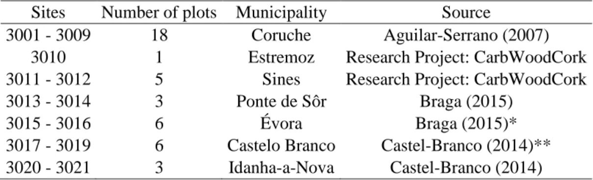
Table 1: Number and location of the plots, and the source of the data measured.

Sites Number of plots Municipality Source

3001 - 3009 18 Coruche Aguilar-Serrano (2007)

3010 1 Estremoz Research Project: CarbWoodCork

3011 - 3012 5 Sines Research Project: CarbWoodCork

3013 - 3014 3 Ponte de Sôr Braga (2015)

3015 - 3016 6 Évora Braga (2015)*

3017 - 3019 6 Castelo Branco Castel-Branco (2014)**

3020 - 3021 3 Idanha-a-Nova Castel-Branco (2014)

*6 plots were measured in 2016 in this thesis. **8 plots were measured in 2016 in this thesis.

Table 2 provides a summary of variables included in the data set and involved in the modelling of the pdf.

17

Table 2: Summary statistics of the data set used for the modeling of the pdf of the

total height. No of measurements = 96.

Variables Units Minimum Mean Maximum

t years 6.00 14.92 22.00 N ha-1 100.00 342.23 730.00 hmean m 0.63 4.01 8.44 hmax m 1.10 6.38 11.30 hmin m 0.15 1.61 5.70 hdom m 1.01 5.53 10.16 S m 11.52 16.51 18.63 SD m 0.14 1.11 1.98 √β1 - -1.16 -0.01 2.06 β2 - 1.53 2.87 11.22 Tmean ºC 14.13 15.63 16.08 Tmax ºC 18.28 21.54 22.48 Tmin ºC 8.52 9.73 13.17 Precipitation mm 493.30 647.08 943.70 Evaporation mm 937.80 1383.17 1957.90 No days precipitation - 65.00 96.66 108.30 Rock depth cm 20.00 102.61 160.00 Soil thickness cm 20.00 92.87 192.00

Surface soil thickness cm 12.00 24.10 40.00

Variables Classes

Soil surface texture A, AF, F, FA, FG, FGA, G

Soil texture A, AF, F, FA, FG, FGA, G

Soil type (FAO) Arenosols, Cambisols, Leptosols, Luvisols

Note: t is the age of the measurement, N is the number of trees per hectare, hmax is

the maximum height, hmin is the minimum height, hdom is the dominant height, S is the site index, Tmean is the mean temperature, Tmax is the mean monthly maximum temperature, Tmin is the mean monthly minimum temperature, Precipitation is the annual precipitation, Evaporation is the annual evaporation, No Days precipitation is the number of days of precipitation, Rock depth is the depth of rock layer, Soil thickness is the soil thickness, Surface soil thickness is the surface soil thickness, hmean is the mean height of the stand, SD is the standard deviation of heights, √β1 is the skewness of the height distribution, β2 is the kurtosis of the height distribution, A is the sandy soil, AF is the sandy loam soil, F is the loam soil, FA is the loamy sand soil, FG is the clay loam soil, FGA is the sandy clay loam soil, and G is the clay soil.

In order to detect and remove eventual extreme observation, the height – diameter relationship was analyzed for each plot and measurement. Tree measurements included in one of the following topics were removed from the data set:

• Trees that didn’t follow the common height – diameter pattern (e.g. trees with stem bifurcation bellow breast height).

18 2.2.Selection of a probability density function

Hafley and Schreuder (1977), based on the work of Hahn & Shapiro (1968), describes a method to assess the flexibility of distributions without the need to estimate any parameters, by means of analyzing the skewness coefficient (

β

The method, also described by Burkhart and Tomé (2012) in chapter 12 and Mateus (2005), allows to choose the proper distribution function that includes: flexibility to describe a broad spectrum of shapes, ease parameter estimation, simplicity of integration methods for estimating proportions in several size classes, and accuracy in fitting the observed data.

Skewness coefficient measures asymmetry, with negative values indicating a distribution with a long tail to the left and positive ones a long tail to the right. Kurtosis coefficient represents the flatness of a distribution: the lower the value of β2 the flatter

the distribution. If the distribution follows the normal pdf, kurtosis coefficient equals to 3 and skewness coefficient to 0. Skewness (

β

computed according to the following equations.

Skewness coefficient 3 1 3 2 2 ( )

µ

β

µ

∑

Even though this procedure does not determine a distribution by itself, it is able to rule out some distribution functions. In order to show the range of kurtosis and skewness coefficients, a graph representing the space of β2 versus β₁ is useful (Figure 2), since

it is able to narrow the seek for distribution functions that describe forest stand height distribution. According to Hahn and Shapiro (1968), there are two main constraints on

19

this methodology: i) the form of a distribution does not only depend on kurtosis and skewness, and consequently the proposed method for the distribution selection doesn’t guarantee a good fit; ii) β₁ and β2 estimators are subjected to fluctuations of sample

nature and thus they will be quite sensitive to extreme observations.

Figure 2:The β₁– β2 space showing the different distributions (Hahn & Shapiro,

1968; Hafley & Schreuder, 1977).

In Figure 2 the normal, exponential and uniform distribution functions, correspond to a single ( β₁; β2) point each: (0;3), (4;9) and (0;1.7), respectively. The log-normal,

gamma, Weibull and Johnson distribution functions are represented in distinct 2D ( β₁;

β2)space, showing the capability to assume a diversity of shapes, and found to be more

flexible since they are represented in a broader segment of the space. In spite of these distributions being quite close in the space to each other, the Weibull and the Johnson’s SB distributions have demonstrated to be the most flexible functions that better fit to

20

forestry data. Some differences among them lie in the ability to represent different types of skewness. While gamma and log-normal distributions represent positive skewness, the Weibull and Johnson ones are able to cover both negative and positive skewness. As Figure 2 shows, the flexible beta distribution encompasses a wide spectrum of shapes, fitting both signs of skewed data, covering the whole region among the gamma distribution line, the β2 axis and the impossible region. Nevertheless, Johnson’s SB

distribution provides rather more flexibility in skewness and kurtosis than the beta distribution (Hafley & Schreuder, 1977).

Johnson’s system includes the space of three distributions: the Johnson’s SL

(lognormal), SB (bounded) and SU (unbounded), that depend on the transformation

applied to the random variable (Johnson, 1949). The advantage of such distributions lies in the fact that the estimators of percentiles of the fitted distribution can be obtained from an accumulative function table of the standard normal distribution. This system presents a great variety of possible shapes. The SB distribution covers the region above

the lognormal line in Figure 2, the SL distribution is a three-parameter lognormal

distribution with one parameter being the lower limit and the SU distribution

encompasses the region below the lognormal line. While the Weibull distribution might not be suitable for all stands regardless of the species composition and silvicultural regime, SB distribution is more flexible and is able to represent bi-modal distributions

(unlike Weibull). In stands with a significant number of small trees, the height and diameter distribution tend to positive skewness and turn gradually into more negative values as the average tree size rises. Seemingly, a few trees with a fast early growth (sprinters) in each stand sets the early positive skewness, while the slow early growers (stayers) convert the skewness into negative values (Cannell & Jackson, 1985).

2.3.Fitting the moments needed to simulate the Johnson’s distribution

The R software (R, 2014) was used to estimate the parameters of the Johnson distribution for each measurement, since it holds several alternative packages that are considered useful for the different task of the thesis. One of these packages encompasses the functions of the Johnson’s systems family (SB, SU and SL), so that it simplifies the

estimation of the parameters (McLeod & King, 2015). This package, named “JohnsonDistribution”, fits the Johnson pdf with the method of moments (Hill et al.,

21

1976; Hill, 1985). To estimate the Johnson’s parameters, the package requires four moments as input: mean height, height standard deviation, skewness and kurtosis. The output provided by the software is a vector including the four parameters that characterize the shape, the range and the location of the Johnson’s probability density function (lambda, delta, epsilon and gamma). The output also provides the identification of the Johnson type most adequate for the data description: SB, SU or SL.

2.4.Modelling the moments needed to estimate the Johnson’s parameters

The next step after choosing the Johnson’s system as the probability density function suitable for total height simulation was the estimation of the parameters characterizing the 96 measurements. For such computation it was necessary to develop models to predict the moments used by the R software to estimate the Johnson’s parameters: mean,

SD,

β

1. Computation and analysis of the correlation scatterplot matrix and Pearson correlation coefficient relating the mean, SD,

β

and edaphoclimatic variables. This also includes the analysis of the relation between the mean, SD,

β

overview of the different relationships between variables and how strong they are. In addition, it shows whether any relationship is not linear and, thus, the type of models to test (linear or nonlinear regression).

2. Perform linear regression analysis, through the usage of the R software (R, 2014), to relate the Johnson’s SD, mean,

β

edaphoclimatic variables. The definition of the best model was made by the “all possible regressions” method (e.g. Myers (1990)), implemented in “Leaps” R software package by Lumley (2015). This method considers all possible subsets of the pool of explanatory variables and finds the linear model that best fits the data according to defined criteria (e.g. Adjusted R2, AIC and BIC). The BIC criteria was used at this step. The models were defined using the linear regression formulation:

22 0 i i i i Y =

β

∑

β

ε

X = Explanatory (independent) variables

o

β

β

ε

3. If the relationship between two of the Yi dependent variables (mean, SD,

β

β2) was evident in the previous steps, suggesting the need for its inclusion in one

of the models as an explanatory variable (Xi), the simultaneous fitting of both models was carried out. This was made with the “systemfit” R software package (Henningsen & Hamann, 2015), by means of the SUR method (Seemingly Unrelated Regression). This method has been demonstrated to provide a benefit in parameter estimation efficiency when the error of equations in the system are correlated (Naesset et al., 2005).

4. Concerning the hmean, the linear model formulation was not considered as the most suitable one. This drives from the fact that it does not guarantee the prediction of positive values, neither the prediction of a hmean value lower to the hdom value of the plot. This implied the need to define a non-linear model that was formulated as:

hmean=hdom− f ( x ) hdom⋅ Eq. 5

Where:

hdom = The dominant height of the stand (m) f(x) = hyperbolic function, varying between 0 and 1

The four hyperbolic models proposed by Paulo and Tomé (2010) were tested, and the one resulting in the lowest MSE was selected. The f(x) function was then expressed as a function of the independent variables that showed to be related to

23

As suggested by de-Miguel et al. (2012), Burkhart and Tomé (2012), and Amaro et al. (2003) the following criteria were considered when evaluating the suitability of the models:

• Consistent with current ecological knowledge

• Parsimony and robustness

• Statistical significance of parameters (p-value < 0.05)

• Absence of bias

• Precision

• Homoscedasticity and normal distribution of residuals

• Absence of collinearity among independent variables

In order to achieve a final model with these characteristics, several statistics were accounted for, such as the summaries that include the p-value for each variable, mean squared error (MSE) and modelling efficiency (ef).

Model efficiency, or the proportion of variation explained by the model, is computed as:

(

)

∑

∑

r = the residual for observation i

i

y = the observed values

y = the mean value

According to Burkhart and Tomé (2012) model error should be assessed in terms of two characteristics: bias and precision. The first refers to the deviation of the average of the model errors from zero and the second to the size of the model errors. Several statistics may be used to assess bias and precision, but the most commonly used are the average model error to assess model bias and the mean absolute difference or mean squared error to assess model precision:

24 Model precision: 2 1 ˆ ( ) n i i i y y MSE n = −

=

∑

Model bias:

(

)

∑

(Average bias) Eq. 8

Where:

p

r = the prediction residual

i

y = the observed values

ˆ_i

y = the predicted values

n = the number of observations in the evaluation dataset

Models must hold absence of collinearity between independent variables, i.e. linear dependencies. Myers (1990) proposes the variance inflation factor (VIF) for the i-th regression coefficient: 2 1 1 i VIF R = − Eq. 9 Where: 2 i

R = the i-th regression coefficient

The VIFs represent the inflation that the variance of each regression coefficient experiences above ideal (Myers, 1990). Although there is no rule about the VIF threshold, it is generally believed that if any VIF exceeds 10, then there is serious collinearity (Myers, 1990).

The homoscedasticity assumption was tested by means of plots of the residuals of each model against the respective predicted values. If the cloud of points is distributed uniformly around zero, the model approach is suitable. This procedure was conducted by the R software packaged so-called “car” (Fox & Weisberg, 2011). The same package was also used to test the normality of residuals assumption, through the analysis of the q-q plots, and to compare the VIFs.

In addition, a complement to the evaluation method was the construction of the graphs of observed versus predicted values together with the (1:1) line that represents

25

discrepancies from perfect fit between simulated and measured values for all models. This allows to observe the bias and precision of the equations. When the model fits well, the dots must be randomly scattered around the (1:1) line which is equivalent to an average of the prediction residuals equal to zero.

2.5.Goodness of fit of the simulated distributions

The final step was to evaluate the goodness – of – fit of the proposed models, and to compare the observed and the simulated total height distributions. For the first purpose, two analyses were carried out to look for some justification for the bad performance of the proposed method in those measurements:

• Plotting of the residuals produced by the developed models as a function of other variables not included as regressors.

• Identification and analysis of the observed pdf associated to unsuitable simulations. Research on additional variables that might characterize these measurements or plots, in order to consider their inclusion in the models. For the purpose of comparing the measured and the simulated total height distributions of the 96 plot measurements, the nonparametric Kolmogorov–Smirnov tests (Dn) was

performed. It allows to compare the cumulative estimated frequency with the observed frequency (Gorgoso-Varela et al., 2008):

1 1 max ( ) , ( ) n i i i n i i D F x F x n n ≤ ≤ −   =  − −    Eq. 10 Where:

F(xi) = Cumulative relative value of the fitted distribution for the height xi

n = Number of observations

The value Dn is compared to the critical value D*_n,α obtained from a table of K–S

according to n and a significance level selected (1% in this case). If Dn is greater than

the critical value, the null hypothesis that the sample population follow the fitted distribution function, is rejected.

26

For each plot measurement the test was carried out 100 times, using the R function called “ks.test” (R, 2014). Each time the K-S test was carried out, it was compared with the measured sample distribution with a different simulated vector that included n random numbers (n being the real number of trees in each plot measurement). These vectors were obtained by the usage of the “yJohnsonDistribution” function, implemented in the R package call “JohnsonDistribution”(R, 2014). This function used as input for characterizing the Johnson’s pdf the estimated parameter values of hmean, SD,

β

β2. In other words, every time that the test is processed, the results are similar but not

absolutely the same due to the differences in those simulated random numbers vectors. The simulation of the total height distribution was considered as an “acceptable” when 80% or more of the K–S tests repetitions hold a p-value equal to or higher than 0.01. When less than 80% of the K–S tests repetitions rejected the null hypothesis that the sample population followed the fitted distribution function, the simulation of that plot measurement was considered “not to be acceptable”. If the proposed value of 80% is altered, different results would be obtained. The results associated to this step are only analyzed as indicators, and would be different if other value was considered. Even so, the value is considered demanding and suitable for the purpose of the thesis.

3. RESULTS AND DISCUSSION

3.1.Selection of a probability density function

Figure 3 and Figure 4 show the range of the estimated

β

-1.16 ≤

β

measurements are distributed mainly along the Johnson SB region, with a reduced

number of observations covering the Johnson SU distribution. This range of values

evidence and support the need of choosing a very flexible distribution.

Analyzing how these values are distributed along the (

β

classes of tree age (Figure 3) allowed to observe that most of the youngest measurements (blue dots: 6 to 10 years old and green dots: 11 to 13 years old) are located in the positive side of skewness, which translates into the higher concentration of the stand height on the left of the distribution graph. This is due to the similar heights taken by the trees at planting age and along the few years that follow, with just a few number of trees presenting higher height values which are represented in the right tail of such

27

distribution graph. On the other hand, measurements taken when the stands have 14 or more years of age (orange dots: 14 to 16 years old and red dots: 17 to 22 years old) show negative values for skewness, with most of the tree heights being higher than the average height. These results are in line with Mateus and Tomé (2011) that analyzed the evolution of diameter distributions of eucalyptus plantations. The eucalyptus that had a small initial growth in diameter continued to have low growth rates, and the differences between sizes tended to increase resulting in negative skewness values. The pattern here described as “the older the stand, the smaller the values of skewness”, is not clear along all plots measurements, presuming due to particular edaphoclimatic conditions that characterize the different stands or different plots inside the same stand. For example, Figure 3 shows some red dots presenting a positive value of skewness even though they are the oldest stands. In particular, this is the case of the measurements taken in the Castelo Branco district, which are characterized by more extreme temperatures and granite soils, and in some plots including waterproof layers that may limit tree root development.

Figure 3: Plot of β1– β2 values of each plot measurement grouped by age classes. The

blue dots belong to the measurements with the youngest trees (6 – 10 years old), the green dots are the measurements with trees of 11 – 13 years, the orange dots are the measurements with trees of 14 – 16 years and the red ones are the measurements with trees of 17 – 22 years.

28

Figure 4 shows the same graph than the previous Figure 3, but with the 96 observations now grouped according to the dominant height. It allows to analyze the evolution of the skewness and kurtosis values along the evolution of dominant height, a variable that better represents the stand development than the stand age variable. Again, blue dots (hdom lower than 4 meters) are located in the positive side of skewness, followed by green dots (hdom from 4.01 to 6 meters) that are distributed around the zero value of

β

than 8.01) that are predominantly located to the left side of the graphic, were negative skewness values are presented.

When considering values of β2, only 2 plot measurements are below 5. Also, no

tendency related to stand age of dominant height prevails since a mixture of dots characterizing different age and dominant height classes is observed.

Figure 4: Plot of β1– β2 values of each plot measurement grouped by hdom class. The

blue dots belong to the measurements with hdom lower than 4 meters, the green dots are the measurements with hdom between 4.01 and 6 meters, the orange dots are the measurements with hdom between 6.01 and 8 meters and the red ones are the measurements with dominant hdom higher than 8.01 meters.

29 3.2.Modelling the moments used to recover the Johnson’s parameters

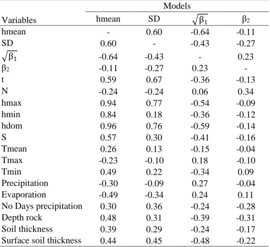
The observation of the values of the Pearson correlation coefficients (Table 3) and the scatter plot correlation matrix (partially shown in ANNEX II) between the variables included in the data set allowed to carry out a first analysis of the relationship between the Johnson’s moments and the stand characteristics. Correlations between the Johnson’s distribution moments and soil variables were analyzed using boxplots graphics (ANNEX III) due to the fact that these are qualitative variables. The results show:

• Mean height (hmean) is linearly and positively correlated to the age of the stand (t), mean monthly minimum temperature (Tmin), dominant height (hdom) and site index (S). In this last case due to its relation with the age and height. When considering the relationship to evaporation, a linear but negative influence is observed with hmean. All these variables were tested for inclusion in the f(x) hyperbolic function as defined in section 2.4.

• Standard deviation (SD) is linearly and positively correlated to age (t) and dominant height (hdom).

• Skewness shows a linear and negative relation to dominant height (hdom), demonstrating that negative values appear in older stands and/or stands characterized by higher hdom.

• In terms of linear relations, Kurtosis only presented a slight relation with the number of trees per hectares (N). Instead, a parabolic relation was observed with the observed value of skewness (

β

• No evident relation between any of the Johnson’s distribution moments and soil variables has been observed. This can derive from the lack of more detailed soil variables such as chemical or physical variables and/or the reduced number of observations taken in some soil classes.

30

Table 3: Pearson correlations coefficients between Johnson’s moments parameters

and the stand characteristics.

Variables Models hmean SD β₁ β2 hmean - 0.60 -0.64 -0.11 SD 0.60 - -0.43 -0.27 β₁ -0.64 -0.43 - 0.23 β2 -0.11 -0.27 0.23 - t 0.59 0.67 -0.36 -0.13 N -0.24 -0.24 0.06 0.34 hmax 0.94 0.77 -0.54 -0.09 hmin 0.84 0.18 -0.36 -0.12 hdom 0.96 0.76 -0.59 -0.14 S 0.57 0.30 -0.41 -0.16 Tmean 0.26 0.13 -0.15 -0.04 Tmax -0.23 -0.10 0.18 -0.10 Tmin 0.49 0.22 -0.34 0.09 Precipitation -0.30 -0.09 0.27 -0.04 Evaporation -0.49 -0.34 0.24 0.11 No Days precipitation 0.30 0.36 -0.24 -0.28 Depth rock 0.48 0.31 -0.39 -0.31 Soil thickness 0.39 0.29 -0.24 -0.17

Surface soil thickness 0.44 0.45 -0.48 -0.22

Note: t is the age at the measurement, N is the number of trees per hectare, hmax is the

maximum height, hmin is the minimum height, hdom is the dominant height, S is the site index, Tmean is the mean temperature, Tmax is the mean monthly maximum temperature, Tmin is the mean monthly minimum temperature, Precipitation is the annual precipitation, Evaporation is the annual evaporation, No days precipitation is the number of days with precipitation, Rock depth is the depth of rock layer, Soil thickness is the soil thickness, Surface soil thickness is the surface soil thickness, hmean is the mean height of the stand, SD is the standard deviation of heights, β₁ is the skewness of the height distribution and β2 is the kurtosis of the height distribution.

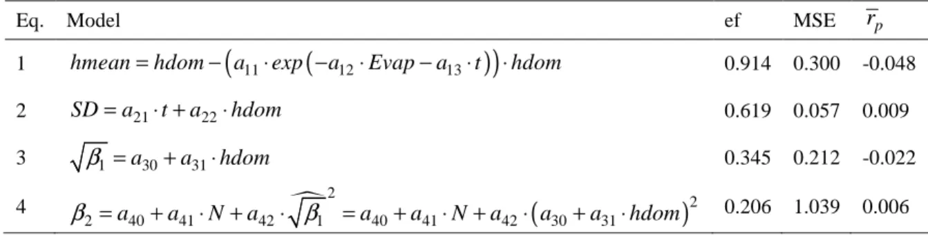
Table 4 presents the final models obtained to simulate the hmean, SD,

β

parameters that characterize the Johnson’s pdf. Two of the models present a linear formulation (SD and

β

statistics show that the mean height and standard deviation models are the ones that present higher values of modelling efficiency (ef). Models for the prediction of skewness and kurtosis show lower values of modeling efficiency. Table 5 shows the parameter estimates of the final models.

31

Table 4: Fitting statistics for the best performing models of the Johnson’s parameters: model efficiency (ef),

the mean squared error (MSE) and the average bias (r_p).

Eq. Model ef MSE rp

1 hmean=hdom−

(

(

)

)

2 SD=a₂₁⋅ +t a₂₂⋅hdom 0.619 0.057 0.009

3 β₁=a₃₀+a₃₁⋅hdom 0.345 0.212 -0.022

4 2

(

)

2 a40 a41 N a42 1 a40 a41 N a42 a30 a31 hdom

β = + ⋅ + ⋅ β = + ⋅ + ⋅ + ⋅ 0.206 1.039 0.006

Note: hmean (m) is the mean height of the stand, SD (m) is the standard deviation of heights, β₁ is the skewness of the height distribution and β2 is the kurtosis of the height distribution, hdom (m) is the dominant height, Evap (mm) is the total annual evaporation, N is the number of trees per hectare, and t (years) is the age of the plantation.

Table 5: Estimated parameters and p-value for the final

models.

Models Coefficients p-value

hmean a11 = 0.2484 ≤ 0.001 a12 = - 0.0003 ≤ 0.01 a13 = 0.0237 ≤ 0.05 SD a21= 0.0334 ≤ 0.001 a22 = 0.1088 ≤ 0.001 β₁ a30 = 0.8916 ≤ 0.001 a31 = - 0.1584 ≤ 0.001 β2 a40 = 1.7597 ≤ 0.001 a41 = 0.0024 ≤ 0.001 a42 = 2.6184 ≤ 0.05

The analysis of the parameter values (Table 5) allowed to discuss the consistency between the models predictions and biological knowledge. The parameter associated to the evaporation in the hmean model (a12) allows to confirm that this variable is

negatively associated to the mean height, while the increase of tree age implies, as expected, an increase of the mean height (a13). These results are in line with the ones

obtained by Paulo et al. (2015b) on the negative effect of evaporation on site index stand value.

The positive value found for the parameter associated to hdom in the SD model (a22)

confirms that the variability between the trees in one stand, here accessed by SD, increases with the stand age. The opposite relation was observed between skewness and

32 hdom, since the negative value estimated for parameter a31, shows older stands tend to

lower skewness values (as explained in the section 3.1).

Finally, the model proposed for the prediction of kurtosis, showed an increase of the kurtosis with both of the values included in the model (N and hdom), since all the parameters present positive values. These relations are difficult to interpret from a biological point of view.

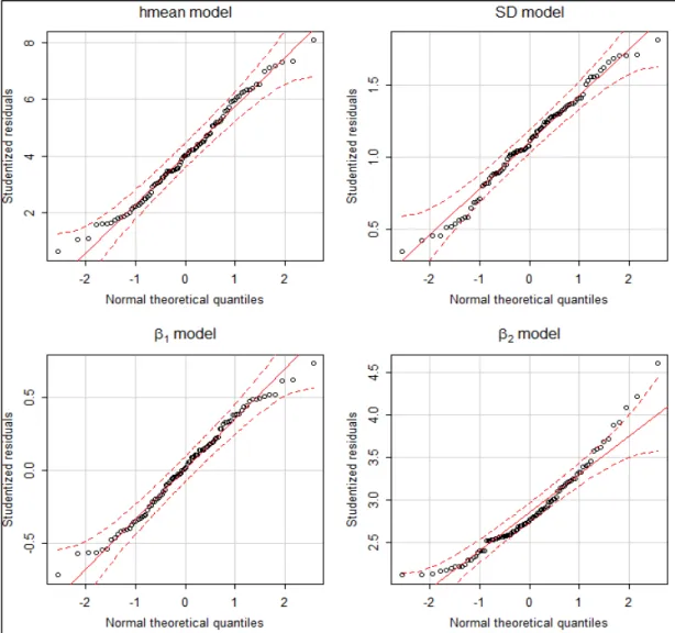
The assumption related to the normality of residuals produced by each of the four models is evaluated in the Figure 5 by means of q-q plots. This figure shows acceptable results for the four models, although it shows some deviation of the residuals resulting from the kurtosis model. This suggests that alternative models can be tested in the future for modeling kurtosis, especially when additional data are collected that allow exploring the relation with other variables and finally increasing modelling efficiency.

33

Considering the final models for the estimation of hmean, SD,

β

presented in Table 4 and Table 5, the simulations of the total height distributions for the 96 plot measurements were carried out (ANNEX IV). The plots include information provided by the output of the R “JohnsonDistribution” package related to the Johnson’s pdf output. In the figures of ANNEX IV the real total height distributions are presented in white bars and the simulated total height distributions in red lines. Two examples are provided in Figure 6: one showing a plot measurement that ‘’has been well simulated’’ (left graph) and others where the simulation does not follow as well the real distribution (right graph).

Figure 6: 2 out of the 96 measurements simulated by Johnson’s distribution with the estimated

moments. The bars are the real distribution and the red line is the Johnson simulation. Gamma, delta, lambda and epsilon are the output parameters of such simulation. Type is the type of Johnson’s family: 1 – SL and 2 – SU. h is the height of the tree in meters.

3.3.Johnson’s parameters validation

Figure 7 provides the graphic of predicted versus observed plots for the four models. It allows to evidence that despite none of the models is biased, models for

β

prediction present low precision in their estimates. The model for the estimation of SD also reveals this characteristic, although more evident for values higher to 1.3. These results are in line with the values of model efficiency presented in Table 4.

34

Figure 7: 1:1 plots between the estimated models and the observed ones.

The results of the K–S test, considering the assumptions made in section 2.5, showed that only 33 out of the 96 measurements should be considered has not acceptable. ANNEX V presents the number of times the K-S test accepted and rejected the null hypothesis for each of the plot measurements. This results indicate an acceptable performance of the framework that was developed in this thesis.

In order to identify the 33 plot measurements where the simulations were considered not acceptable and to look for additional relations between the hmean, SD,

β

other variables not included in the final models proposed, Figure 8 and ANNEX VI were carried out. They present the relationship between the residuals of each model and several stand variables tested in the modelling process. As no evident pattern is shown in these graphics, the available variables are not expected to contribute further for the modeling of the parameters that characterize the Johnson’s pdf. Alternatively, additional variables related to chemical and physical soil properties and/or annual climate variables characterizing the period between the stand plantation and the measurements are suggested to be collected and explored in order to improve the models and the simulations of the total height distribution of young cork oak stands.

35

Figure 8: Plots of the residual versus the independent variables of each model. The red dots identify the

36

4. CONCLUSION

The main conclusions of this dissertation are:

1. The Johnson’s distribution is an appropriate probability density function to simulate de height distribution of young cork oak stands. Its flexibility allows to encompass the different shapes of the distributions defined mainly by the kurtosis and skewness.

2. It was possible to model the four moments needed to estimate the Johnson’s parameter with the method of moments. The scatterplot matrix and the “all possible regressions” helped in the definition of the regressors and the type of relationship. The standard deviation is predicted with a linear regression on

hdom and t, the skewness with a linear regression on hdom, the kurtosis with a

nonlinear regression of the skewness and N, and the mean height with a nonlinear regression on hdom, evaporation and t.

3. The mean height model presents a low value of MSE and the highest modelling efficiency value; the kurtosis is the one with the poorest performance according to the same statistics.

4. 66% of the simulated distributions are in accordance to the observed ones according to the K-S test (p-value of 0.01).

5. 34% of the distributions simulated significantly differ from the observed ones according to the K-S test (p-value of 0.01). No pattern explains this behavior. 6. The general behavior of the Johnson simulation from the moments predicted

with the four models proposed is quite acceptable to predict height distributions for new cork oak plantations as those already established.

Further work needs to be done to gather more data, in order to fill the lack of soil information related to some variables (e.g. chemical and physical soil variables) for some of the plots used in this study, and to expand the temporal resolution of the permanent plot equally between them, allowing the development of models that are more robust than the ones presented here.

37

5. REFERENCES

1. Aguilar-Serrano, T. (2007). Análisis de la distribución de alturas en alcornoques en

fase de regeneración. Master thesis. Instituto Superior de Agronomia. Universidade

Técnica de Lisboa. Lisboa.

2. Amaro, A., Reed, D., & Soares, P. (2003). Modelling forest systems. Lisbon. Portugal: CABI.

3. APCOR. (2015). Sustentabilidade social e económica. Retrieved April 5, 2016, from http://www.apcor.pt/montado/sustentabilidade/sustentabilidade-social-e-economica/ 4. Braga, F. M. de C. (2015). Modelação do crescimento em altura e da relação

diâmetro-altura de árvores jovens de Quercus suber. Master thesis. Instituto

Superior de Agronomia. Universidade Técnica de Lisboa. Lisboa.

5. Burkhart, H. E., & Tomé, M. (2012). Modeling forest trees and stands. New York: Springer Science & Business Media.

6. Cannell, M. G. R., & Jackson, J. E. (1985). Attributes of trees as crop plants. California: Institute of Terrestrial Ecology.

7. Cao, Q. V. (2004). Predicting parameters of a weibull function for modeling diameter distribution. Forest Science, 50(5), 682–685.

8. Castel-Branco, D. A. A. da S. (2014). Análise da mortalidade em plantações jovens

de sobreiro (Quercus suber L.) e sua relação com a qualidade da estação. Master

thesis. Instituto Superior de Agronomia. Universidade Técnica de Lisboa. Lisboa. 9. Clutter, J. L., & Bennett, F. A. (1965). Diameter distributions in old-field slash pine

plantations. Georgia: Georgia Forest Research Council.

10. Coelho, M. B., Paulo, J. A., Palma, J. H. N., & Tomé, M. (2012). Contribution of cork oak plantations installed after 1990 in Portugal to the Kyoto commitments and to the landowners economy. Forest Policy and Economics, 17, 59–68. http://doi.org/10.1016/j.forpol.2011.10.005

11. de-Miguel, S., Pukkala, T., Assaf, N., & Bonet, J. A. (2012). Even-aged or uneven-aged modelling approach? A case for Pinus brutia. Annals of Forest Science, 69(4), 455–465.

38

relación altura-diámetro para Pinus pinaster Ait. en Galicia mediante la función de densidad bivariante S BB. Invest. Agr. Sist. Recur. For., 10(1), 111–125.

13. Faias, S. P., Palma, J. H. N., Barreiro, S., Paulo, J. A., & Tome, M. (2012). Resource communication. sIMfLOR - platform for portuguese forest simulators. Forest

Systems, 21(3), 543–548. http://doi.org/DOI 10.5424/fs/2012213-02951

14. Fonseca, T. F., Marques, C. P., & Parresol, B. R. (2009). Describing maritime pine diameter distributions with Johnson’s SB distribution using a new all-parameter recovery approach. Forest Science, 55(4), 367–373.

15. Fox, J., & Weisberg, S. (2011). R package: An {R} Companion to Applied Regression. Retrieved from https://cran.r-project.org/web/packages/car/index.html 16. García Güemes, C., Cañadas, N., & Montero González, G. (2002). Modelización de

la distribución diamétrica de las masas de“ Pinus Pinea” L. de Valladolid (España) mediante la función Weibull. Investigación Agraria. Sistemas Y Recursos Forestales,

11, 263–282.

17. Gorgoso, J. J., Rojo, a., Cámara-Obregón, a., & Diéguez-Aranda, U. (2012). A comparison of estimation methods for fitting Weibull, Johnson’s SB and beta functions to Pinus pinaster, Pinus radiate and Pinus sylvestris stands in northwest Spain. Forest Systems, 21(3), 446–459. http://doi.org/10.5424/fs/2012213-02736 18. Gorgoso-Varela, J. J., García-Villabrille, J. D., & Rojo-Alboreca, A. (2015).

Modeling extreme values for height distributions in Pinus pinaster, Pinus radiata and Eucalyptus globulus stands in northwestern Spain. iForest - Biogeosciences and

Forestry, 008(1927), e1–e7. http://doi.org/10.3832/ifor1447-008

19. Gorgoso-Varela, J. J., García-Villabrille, J. D., Rojo-Alboreca, A., Gadow, K. Von, & Álvarez, J. G. (2016). Comparing Johnson ’ s SBB , Weibull and Logit-Logistic bivariate distributions for modeling tree diameters and heights using copulas. Forest

Systems, 25(1), 1–5.

20. Gorgoso-Varela, J. J., Rojo-Alboreca, A., Khouro, E., Barrio-Anta, M., Afif-Khouri, E., & Barrio-Anta, M. (2008). Modelling diameter distributions of birch (Betula alba L.) and pedunculate oak (Quercus robur L.) stands in northwest Spain with the beta distribution. Forest Systems, 17(3), 271–281.