1
Deployment characterization of a floatable tidal energy converter on a tidal
1channel, Ria Formosa, Portugal
2Pacheco, A.1, Gorbeña, E.1, Plomaritis, T.A.1, Garel, E.1, Gonçalves, J.M.S.2, Bentes, L.2, 3
Monteiro, P. 2, Afonso, C.M.L.2, Oliveira, F.2, Soares, C.3, Zabel, F.3, Sequeira, C.1 4
1CIMA, University of Algarve Ed7, Campus de Gambelas 8005-139 Faro, Portugal
5
2Centro de Ciências do Mar (CCMAR), University of Algarve, Campus de Gambelas, 8005-139 Faro, Portugal
6
3MarSensing Lda., Centro Empresarial Gambelas Campus de Gambelas Pavilhão B1, 8005-139 Faro, Portugal
7 8 Doi: https://doi.org/10.1016/j.energy.2018.06.034 9 Abstract 10
This paper presents the results of a pilot experiment with an existing tidal energy converter 11
(TEC), Evopod 1 kW floatable prototype, in a real test case scenario (Faro Channel, Ria 12
Formosa, Portugal). A baseline marine geophysical, hydrodynamic and ecological study based 13
on the experience collected on the test site is presented. The collected data was used to validate 14
a hydro-morphodynamic model, allowing the selection of the installation area based on both 15
operational and environmental constraints. Operational results related to the description of 16
power generation capacity, energy capture area and proportion of energy flux are presented 17
and discussed, including the failures occurring during the experimental setup. The data is now 18
available to the scientific community and to TEC industry developers, enhancing the 19
operational knowledge of TEC technology concerning efficiency, environmental effects, and 20
interactions (i.e. device/environment). The results can be used by developers on the licensing 21
process, on overcoming the commercial deployment barriers, on offering extra assurance and 22
confidence to investors, who traditionally have seen environmental concerns as a barrier, and 23
on providing the foundations whereupon similar deployment areas can be considered around 24
the world for marine tidal energy extraction. 25
Keywords: Tidal energy; Tidal energy converters; Floatable tidal turbines; Energy production;
26
Ria Formosa, Portugal. 27
2
1. Introduction
28
The hydrokinetic energy that can be extracted from tidal currents is one of the most promising 29
new renewable energy technologies [1]. Despite its huge potential, energy extraction from tidal 30
energy converters (TEC) devices is still in its infancy. The prospects for tidal energy converter 31
technologies very much depend on the specific device concept and how those devices can be 32
optimised to efficiently extract energy, minimizing environmental impacts. Science currently 33
has a very poor understanding of both the hydrodynamics and the ecological implications 34
related with the extraction of energy on coastal environments. In few cases where devices have 35
been deployed the data is highly commercially sensitive and thus not in the public domain and 36
available to the scientific community for research development. The deployment of TECs has 37
also been hindered by a lack of understanding of their environmental interactions, both in terms 38
of the device impact on the environment (important for consenting and stakeholder bodies) and 39
environmental impact on the device (fatigue, actual power output, etc.) which is vital to 40
enhance investor confidence and increase financial support from the private sector. The access 41
to freely available, transparently collected monitoring data from real deployments is paramount 42
both for resource assessments and for cataloguing potential impacts of any marine renewable 43
installation. 44
This paper presents the results from the deployment of a small-scale tidal current turbine 45
(Evopod E1) in a shallow-water estuarine environment, Ria Formosa Portugal, under SCORE 46
project Sustainability of using Ria Formosa Currents On Renewable Energy production. This 47
1:10th scale prototype operated from June to November 2017. The general objective of SCORE 48
is to construct an operational envelope, which can be used by technology developers for design 49
concepts of efficient TECs based on environmental and sustainability principles, contributing 50
to the growth of the blue economy. The deployment site and prototype characteristics are 51
presented in sections 2; section 3 presents the challenges on installing, operating and 52
decommissioning E1 prototype, along with the data collected under the monitoring program; 53
section 4 presents the results obtained, which are fully open access and available for download, 54
following the European Marine Energy Centre (EMEC) standards; and section 5 draws the 55
final remarks and describes ongoing work. 56 57 2. Experimental settings 58 2.1. Deployment site 59
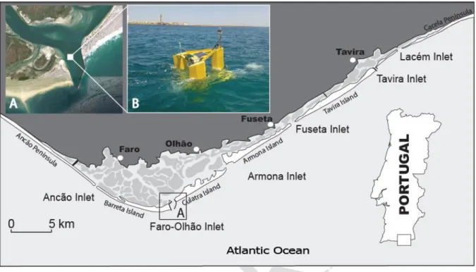
3 The experience with the TEC prototype was performed at Faro-Olhão Inlet, the main inlet of 60
Ria Formosa system (hereafter RF), a coastal lagoon located in the South of Portugal (Figure 61
1). The RF is a multi-inlet barrier system comprising five islands, two peninsulas separated by 62
six tidal inlets, salt marshes, sand flats and a complex network of tidal channels. The tides in 63
the area are semi-diurnal with typical average astronomical ranges of 2.8 m for spring tides and 64
1.3 m for neap tides. A maximum tidal range of 3.5 m is reached during equinoctial tides, 65
possibly rising over 3.8 m during storm surges. The wind is on average moderate (3 ms 1) and 66
predominantly from the west. Variance analysis of both tidal and nontidal signals has shown 67
that the meteorological and long-term water-level variability explains less than 1% of the total 68
recorded variance [2]. The lagoon is generally well mixed vertically with no evidence of 69
persistent haline or thermal stratification, which relates to the reduced freshwater input and 70
elevated tidal exchanges i.e. the lagoon is basically euryhaline with salinity values close to 71
those observed in adjacent coastal waters [3]. 72
The deployment site was selected nearby the navigation channel of Faro-Olhão Inlet, Faro 73
Channel, the largest and most hydraulically efficient channel of RF. The depths of the channel 74
in the deployment area range between 4 and 15 m (below msl). Faro-Olhão Inlet is the main 75
inlet of the system, trapping 60% of the total spring-tidal prism of the RF system [4]. The inlet 76
is characterised by strong currents (depth average velocities over 2 ms-1 at the inlet throat),
77
especially during ebb. A large difference between flood and ebb duration occurs during spring-78
tides i.e. ebb duration is shorter and mean velocities are higher. This difference becomes 79
smaller during neap-tides. Due to the narrow inlet mouth (Figure 1A) and the strong tidal 80
current, limited offshore wave energy is reaching the lagoon. Nevertheless, the mooring 81
location could experience fetch dependant waves generated by wind blowing over the lagoon 82
water from the NW or NE directions. 83
Energy from tides was harvested before at Ria Formosa with tidal mills (XII century) and recent 84
tidal energy assessments determined a mean and maximum potential extractable power of 0.4 85
kWm-2 and 5.7 kWm-2, respectively [5]. The RF has attracted research interest in all 86
environmental aspects and hence there is a lot of background literature available about biology, 87
morphodynamics and hydrodynamics. The system is particularly adequate for testing floatable 88
TEC prototypes, and representative of the vast majority of transitional systems where these 89
devices can be used to extract energy to power small local communities. 90
4
2.2. E1 Evopod 1 kW prototype
92
Evopod™ is a device for generating electricity from coastal tidal streams, tidal estuaries, rivers 93
and oceanic sites with strong currents (Figure 2). It is a unique floating solution drawing upon 94
proven technologies used in the offshore oil/gas and marine industries [6]. The 1:10th scale 95
Evopod (E1 hereafter) consists of a positively buoyant horizontal cylindrical body of 2 m 96
length and 0.4 m diameter to which are attached three stabilising fins set in a triangle, tethered 97
to a subsurface buoy. Each fin is approximately 1.2 m height, 0.4 m wide and 0.1 thick. The 98
main body and fins are constructed of steel. When deployed, approximately 0.4 m of the fins 99
are above the water surface. The semi-submerged nacelle has surface piercing struts providing 100
sufficient reserve of buoyancy to resist to the vertical component of the drag force produced 101
by the moorings. The surface piercing struts have a small water-plane area so that the motions 102
of E1 in waves are minimised and do not adversely affect the turbine performance. 103
A four-bladed 1.5 m diameter turbine made of composite material is attached at the rear of the 104
body and is designed to rotate between 20 and 55 rpm. This result on a maximum blade tip 105
speed of 4.3 ms-1, driving a 1 kW permanent magnet AC generator at a rated flow velocity of 106
1.7 ms-1. E1 has a cut-in velocity of 0.7 ms-1 and it cannot withstand steady flow velocities 107
larger than 1.75 ms-1. The width of each blade is approximately 0.1 m and the depth between
108
the sea surface and the highest point of the rotor is 0.45 m. Hence, the E1 device consists of a 109
fixed pitch 4-bladed turbine driving through a step-up planetary gearbox to a 3-phase multipole 110
permanent magnet generator. The power from the generator feeds a navigation beacon plus an 111
extensive suite of instrumentation measuring the flow speed, voltage, current, torque, revs, 112
temperature, resistor settings, yaw angle and mooring tension. Data records are logged 113
internally and transmitted to a remote PC through GSM communication. Table 1 summarises 114
Evopod™ key discriminators at different scales. 115
116
3. Methodology
117
3.1. Deployment, operation and decommissioning
118
The E1 deployment took place on 8th June 2017. Authorization for deployment was obtained 119
from local maritime authorities following a fast and simple administrative procedure. The 120
device was tethered to the seabed using a four-line catenary spread mooring system 121
(Figure 3A). The flow speeds, wave and wind characteristics at the deployment site were used 122
for the design of the mooring system (Table 2). The moorings consists of chain and galvanised 123
5 wire mooring lines attached to 4 concrete anchors weighting approximately 1 ton each 124
(Figure 3C). The device is a simple fixed pitch downstream turbine, which aligns freely with 125
the predominant current direction. A load cell was placed for the two south and north lines 126
(Figure 4A), respectively, measuring the tension while E1 is extracting energy. Since the 127
prototype has been deployed for three months, it was not connected to the grid and therefore 128
the excess generated power was dissipated as heat into the sea. 129
The prototype was installed in collaboration with a local marine services company, which was 130
subcontracted to provide a barge boat equipped with a winch (Figure 4B), essential to lower 131
the anchoring weights at their exact planned location, using RTK-DGPS positioning. The 132
operation was performed at slack tide and involved a staff of ten people, including skippers, 133
researchers, divers and technical operators, supervised by the maritime authorities. The 134
prototype operated at site (Figure 4C) until the 21st November, when it was towed back to the 135
harbour and removed from the water. All the anchoring system was removed except the 136
anchoring weights that remained on site. 137
138
3.2. Data collection
139
3.2.1. Defining deployment location
140
Prior to the deployment a baseline marine geophysical, hydrodynamic and ecological database 141
for the pilot site was created. Table 3 summarises the data obtained under SCORE project. The 142
first step of data collection was to complement existent LiIDAR bathymetric data of RF and 143
refine the depths at the deployment site. For this task, bathymetric data (Figure 5A) were 144
collected using a single beam eco-sounder (Odom Hydrographic System, Inc. with a 200 kHz 145
transducer) synchronized at 1 Hz with a RTK differential GPS (rover unit model, Trimble R6), 146
though a computer interface running hydrographic survey software (Hypack® 2011, Coastal 147
Oceanographics, Inc.). This allows correcting in real time the tidal and surge levels. A side 148
scan sonar (Tritech StarFish 452F, 450 kHZ) survey was performed to evaluate the presence 149
of priority habitats and characterise the bottom of the deployment area in terms of substrate 150
and the texture type. This characterization allowed the detection of rocky and sediment areas 151
that might be present in the area permitting to choose the best sampling technique for habitat 152
characterization on each bottom type detected. 153
To fully characterise the 3D flow pattern at the deployment location, an ADCP (Nortek AS 154
Signature 1 MHz) was bottom mounted at a mean water depth of 7.7 m (Figure 5B). Current 155
6 velocities were measured with 0.2 m cell resolution through the water column, measuring 60 s 156
of data every 5 min bursts. One of the main objectives of the current velocity data collection 157
was to set-up, calibrate and validate a vertical averaged hydrodynamic model (Delft3D) of the 158
entire RF [more details on modelling setup are given on 7], to define the extraction potential at 159
the test case site and to confirm that the deployment location satisfies the prototype constrains 160
(Table 2). From Figure 6, it is evident that flow velocities constraints restricted the locations to 161
place the device. The selected area was then target of a more refine characterisation of current 162
velocities to fully characterize the 3D flow patterns at the deployment location during complete 163
tidal cycles. Those measurements were performed with a Sontek ADCP 1.5kHz with bottom 164
tracking (Figure 5B) by mooring the boat at the exact deployment location (red cross, Figure 165
6). Velocity components were measured along cells of 0.5 m through the water column, by 166
collecting velocity profiles at each 5 s. Based on those measurements, the estimated E1 167
electrical power outputs, Pe, were calculated using Equation 1:
168
𝑃𝑒 =1
2𝜌𝜂𝐶𝑝𝐴𝑇𝑈𝑟_𝑎𝑣𝑔
3 (1)
169
where, ρ is sea water density (1025 kgm-3); η represents generator efficiency, gear losses and 170
shaft losses (90%, 5% and 5%, respectively); Cp is the power coefficient (28% [5]); AT is the
171
rotor swept area; and Ur_avg represents the flow speed averaged through E1’ rotor swept area
172
i.e. by integrating the ADCP velocity measurements along the area through which the rotor 173
blades of the turbine spin. 174
175
3.2.2. Environmental site Characterisation
176
Several underwater data acquisition methods were tested to identify their viability of use in a 177
high current condition. The techniques employed should give an overview of the priority 178
habitats and communities of species present in the testing area (Figure 5B). Tested sampling 179
methods included: (1) collection of sediment using a "Van Veen" type grab – intended for the 180
quantification and identification of invertebrate species of infauna and also of epibenthic 181
species that are buried in the sand; (2) bottom trawling with a beam-trawl, following the Water 182
Framework Directive’s standards [8], which allowed the quantification of epibenthic species 183
(fish and macroinvertebrates) on mobile substrates; (3) underwater visual censuses (UVC) 184
through transects with SCUBA diving, for the identification and quantification of epibenthic 185
fish and invertebrate on mobile substrates; and (4) video transects with Remote Operating 186
7 Vehicle (ROV, SEABOTIX L200 equipped with two forward-facing cameras), which was used 187
to identify/quantify epibenthic habitats and species through the analysis of videos collected 188
during each immersion of the underwater vehicle. Moreover, the interactions between marine 189
mammals, marine turtles, seabird and fish with the turbine were evaluated through visual 190
census and the colonization of the mooring system was assessed by visual inspection of 3 fixed 191
quadrats (10x10 cm) in two opposite anchoring weights (3x3 photoquadrats). 192
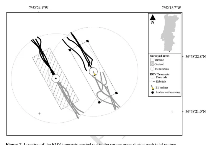
The ROV video sledge was used to characterize an impact zone of 60 x 15 m centred in the 193
tidal turbine. The impact zone refers to the area where the device was deployed i.e. the spatial 194
area limited by the four mooring weights and lines connected to the E1. In this area two 40 m 195
transects were carried out, one during the flow tide and another during the ebb tide (Figure 7). 196
The same procedure was carried out in a control zone, located 50 m apart from the turbine’ 197
deployment area, at the same depth range, bottom type and similar hydrodynamic conditions. 198
Transects were perform at low speed (< 1 knot) with the navigation being monitored with 199
differential GPS. The study areas (i.e. impact and control) were surveyed in four time intervals: 200
3 days prior to the deployment (T-3), and 8 days (T+8), 15 days (T+15) and 63 days (T+63) 201
after the turbine had been installed. Wildlife interaction with the turbine were observed using 202
the same schedule. 203
Video images collected were annotated using COVER software (Customizable Observation 204
Video Image Recorder, v0.7.2) [9]. Every linear meter a still image was used to visually 205
estimate and quantify the percent-cover of the arborescent bryozoan Bugula neritina using 206
ImageJ 1.51j8 [10]. Three additional Gopro cameras were also attached to the video sledge, at 207
70 cm from the bottom, one central facing downward and two in each side at a 45° angle, with 208
the purpose of creating an orthophotomosaic of the seabed. Benthic invertebrates are often 209
selected as indicators of marine monitoring, because of their sessile nature and life strategies, 210
macrobenthos responds moderately rapidly to anthropogenic or natural disturbances [11]. 211
During the pilot study, B. neritina had been identified as a structural component of the benthic 212
community, so the cover percentage of this species was defined as a proxy of the potential 213
disturbances affecting the local fauna. B. neritina was also chosen as a target species due to 214
their high abundance, sessile nature and easiness of identification from still images. 215
Prior to the installation of E1, a baseline measurement of noise level was performed in January 216
2017. The acoustic data was collected with an autonomous hydrophone, the digitalHyd SR-1, 217
installed on a tripod structure (Figure 5C) at a water depth of approximately 11 m, for 13 full 218
8 days. A similar acquisition procedure was repeated during the device operation for an interval 219
of 19 full days in August 2017. In both occasions, the equipment was set to record 90 s of 220
acoustic data every 10 minutes, over a frequency band from 0 to approximately 24 kHz. The 221
data analysis consists in obtaining estimates of sound pressure levels (SPL) over the entire 222
acquisition interval, mainly based on statistical indicators both for broadband sound pressure 223
level (SPL) and frequency levels. In November 2017, a complementary data recording was 224
carried out during half of a tide cycle from a boat, by displacing the boat from a flow line 225
passing the rotor. 226
227
3.2.3. Device performance data
228
The E1 is instrumented to continuously monitor and log various parameters. The parameters 229
captured during the RF deployment were: flow speed (ms-1), shaft speed of rotation (RPM), 230
generator output voltage (Volts) and current (Amps), device compass heading (º degree) and 231
mooring tension (kN). The flow speed past the nacelle was measured using an Airmar CS4500 232
ultrasonic speed sensor. A C100 fluxgate compass from KVH Industries Inc provided compass 233
heading; while mooring tensions, FT, were measured using 0-5kN load cells supplied by
234
Applied Measurements Ltd. 235
The above analogue data streams were logged using a Squirrel data logger from Grant 236
Instruments. A two-level gear system was installed in order to reduce the shaft speed during 237
high current velocities. The logger has an alarm feature used to control the load on the generator 238
by switching in and out additional resistors. The timing of the gear changes are logged in the 239
system. The base load resistance on the tidal turbine is a battery charger that is used to maintain 240
charge in the on board battery which powers the logger and instrumentation. This tidal turbine 241
battery charging was supplemented by solar panels. The logger set-up allows specifying 242
different sampling rates and logging intervals. At the beginning, the logger was set to record at 243
1 Hz. After changing the batteries and solar panels, the acquisition rate was changed to 0.1 Hz 244
to the logger’ extend power capacity. The only exception was the flow speed sensor, which 245
sampled always at 5 Hz. 246
The turbine performance data were then read based on the recorded timestamp. First, the time-247
series were checked for duplicate times and for inconsistences in the recording time step (i.e. 248
from 1 to 10 sec). Common occurring phenomenon could inflict time drifting of the recording 249
parameters at slightly different timestamps. To counter the aforementioned problem, all 250
9 parameters were interpolated on a common and fixed time step of 10 sec. Second, all recorded 251
parameters were transformed from the measured quantity (Volts) into the correct units using 252
the calibration equations. Finally, the generated time series were smoothed by applying a 253
moving average filter. 254
The thrust coefficients, CT, were calculated using load cells data using Equation 2:
255 𝐹𝑇 = 𝐹𝑇,𝑜+ 1 2𝜌(𝐶𝑇𝐴𝑇+ 𝐶𝑠𝐴𝑠)𝑈𝐸1 2 (2) 256
where, FT,o depicts the tension force measured by load cells at rest (i.e. at 0 ms-1); Cs is the drag
257
coefficient of E1 structure (~ 0.15 [6]); As is the E1 cross-sectional area (~1.15𝐴𝑇); and UE1
258
represents the flow speed measured by E1’ on-board mounted Doppler. Using the load cells 259
data, the CT for E1 is obtained by fitting a quadratic drag law of the form 𝑦 = A𝑥2 + b, where
260 y = FT , b = FT,o, x = UE1; and 𝐴 = 1 2𝜌(𝐶𝑇𝐴𝑇+ 𝐶𝑠𝐴𝑠). 261 262 3.2.4. Wake measurements 263
Wake downstream of E1 was characterized at different distances downstream of the channels 264
by combining the use of two ADCPs (Nortek Signature 1 MHz and Sontek ADP 1.5 kHz; 265
Figure 3A). The objective of the wake measurements was to construct the velocity field near 266
the E1 in order to detect, if possible, the spatial characteristics of the wake over different tidal 267
stages, currents velocities and rotor velocities. Those measurements were made for complete 268
tidal cycles using two different techniques: (1) continuous boat-mounted transects; and (2) 269
static measurements at fix positions along the flow axis (Figure 3). 270
On (1), the boat was manoeuvred through pre-defined lines spaced every 5 m from the rotor 271
until 30 m distance. Measurements were performed using a Sontek ADP 1.5 kHz with bottom-272
tracking and sampling at continuous mode (e.g. sampling a profile every 5 s). The boat speed 273
was set to the minimum possible in order to assure the best possible data density; but high 274
enough to sample the full area in less than 10 min to assure stationary flow conditions (i.e. 275
constant tidal current). Each set of data was measured at 30 min in order to characterise the 276
spatial and temporal distribution of the wake during the peak flood. This resulted in a total 277
number of 9 timestamps during the 3 hours period around the peak flood. A constant vertical 278
grid was created from 1.1 m depth (i.e. first measured valid cell) up to the maximum water 279
depth with a 0.3 m resolution. 280
10 On (2), the boat was used as a floatable platform i.e. the Nortek Signature 1 MHz was operated 281
from the boat by displacing the boat from a flow line passing the rotor (i.e. rotor tail and/or 282
wake centre), collecting measurements every 5 s during 5 min bursts. With an ADCP draft of 283
0.1 m, a blanking distance of 0.1 m and a cell size of 0.2 m, the first reading is at a 0.3 m depth 284
and the last at 4.5 m depth. This set-up allowed characterizing the vertical profile of E1’s wake, 285
which its centreline is at an approximate distance of 1.5 m from the free surface (i.e. 286
approximately the rotor centre). A total of 8 complete sets of wake profiles were measured. 287 288 4. Results 289 4.1. Deployment location 290
A bathymetric map of the entire Ria Formosa has been built and is provided on the database 291
(http://w3.ualg.pt/~ampacheco/Score/database.html) as netcdf file using the high resolution 292
LiDAR bathymetry performed on 2011, coupled with bathymetric data from the Faro Port 293
Authority and with 2016’ bathymetric surveys performed under the SCORE project. The 294
database also provides the mosaic from the side scan survey where main morphological 295
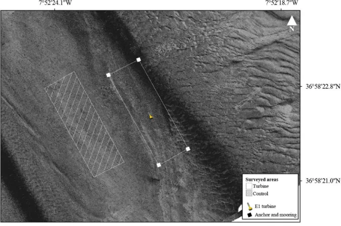
features can be distinguished (i.e. ripples and mega-ripples). An area of about 6 hectares was 296
surveyed using the side scan sonar technique, revealing a seabed mainly composed of sand, 297
coarse sediments and gravel with a high biogenic component (Figure 8). 298
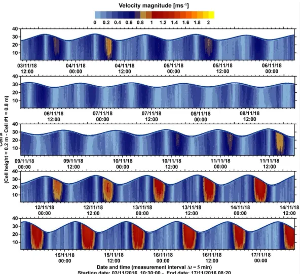
Figure 9 shows the vertical profiles of the computed horizontal velocity magnitudes observed 299
for a 14 days interval using the Nortek AS Signature 1 MHz. It is evident the tidal current 300
asymmetry that takes place in the Faro-Olhão Inlet, with ebb currents being significantly 301
stronger than flood currents. This result is important since even modest tidal asymmetry can 302
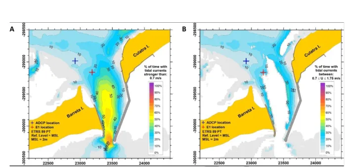
cause large power asymmetry [12]. These velocity measurements allowed validating the 303
Delft3D model and to select the E1 deployment location (Figure 6). The red cross on Figure 6 304
marks the E1 deployment site which meets the velocity criteria (velocity range between 0.7 305
and 1.75 ms-1) for around 21% of fortnight cycle. Subsequently, velocity measurements were 306
performed during a spring ebb tide at the deployment location with the ADP Sontek 1.5 kHz, 307
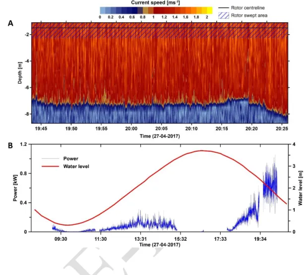
with bottom tracking. Figure 10A shows an example of a time-series contour map of the peak 308
ebb currents at the deployment site, permitting to identify the maximum tidal current velocities 309
that E1 could be exposed; while Figure 10B presents an estimation of the predicted power 310
output using Equation 1. Overall, velocity maximums exceeded the threshold value of 311
~1.75 ms-1 at specific cells, reaching up to ~1.96 ms-1. However, the limit was not surpassed 312
11 when those cell velocities were averaged by the rotor diameter at time intervals of 5 s, resulting 313
on a maximum averaged flow velocity of ~1.68 ms-1. It can be observed that the rated E1
314
capacity is almost achieved at peak ebb (~1 kW, Figure 10B), whereas observed power 315
fluctuations are related to turbulence and eddies propagation. 316
317
4.2. Environmental site characterization
318
Several limitations were identified in the methods tested. Bottom trawl showed handling 319
limitations in the turbine’ deployment area and since this method needs a minimal operation 320
area it would not allow any impact zonation. Bottom trawl is also an extractive technique and 321
therefore not suitable to assess cumulative impacts over time with successive sampling in a 322
small area. Also, as the study area is located in a Natural Park the use of this method was 323
considered the least appropriate. However, the species list provided was the most 324
comprehensive of all methods tested. Thus, surveys were made just for the characterization of 325
the general study area, ensuring the existence of a reference base species list. 326
Species inventory from UVC accounted for 31 different species. The epibenthic invertebrate 327
and fish communities were composed of typical and frequent organisms in the soft substrates 328
of Ria Formosa, such as: Octopus vulgaris, Bugula neritina, Pomatoschistus microps, 329
Holothuria arguinensis, Alicia mirabilis, Sphaerechinus granularis or Trachinus draco. As
330
expected, strong currents made almost impossible the use of UVC through linear transects. 331
However, this was the only method that have detected a seahorse species that is a vulnerable 332
species. Therefore, random transects were done in the specific study area, mainly for species 333
inventory and collection and for ground-truthing ROV data. The strong currents also made 334
extremely difficult to be precise in the location of dredge’s samples for the environmental 335
characterization. Later on, during the operational interval, the high hydrodynamism, the rough 336
bottom and the small area to be sampled implied the increase of deployments; given the low 337
efficiency of the technique in such conditions (2 out 3 deployments were rejected/invalid). 338
Furthermore, the analysis of the samples require several taxonomy expertise, which is more 339
time and money consuming. 340
Using the ROV in high current areas proved to be a difficult operation. To counteract this 341
problem, the ROV was attached to a sledge and towed along the seabed. This would allow a 342
better control while conducting linear transects and provided a stable platform for additional 343
cameras to be attached. The advantages of ROV compared to regular video cameras are mainly 344
12 related with its dynamic operability namely the possibility of making adjustments in real time 345
(zooming, changing angles and controlling the light intensity) and the main disadvantages are 346
the initial investment in equipment and piloting skills. Due to this preliminary analysis, it was 347
concluded that for the general environmental and impact assessment the use of ROV/video 348
cameras in a sledge was the most appropriate technique because it was the most practical and 349
non-destructive technique available. 350
A total of 640 images were annotated thoroughly for the presence and quantification of the 351
coverage of the seabed by B. neritina. Percent-cover of this species ranged from 0 to 39.7% 352
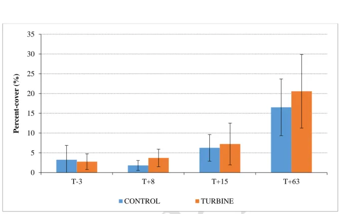
(mean: 7.8%) taking into account all images analysed. Mean values of seabed cover increased 353
similarly over time in both survey areas (Figure 11), with slight higher mean values taking 354
place in the turbine area. Percent-cover was found to be significantly different across time in 355
the turbine (Kruskal-Wallis ANOVA on Ranks: H = 169.253; P<0.001) and in the control 356
(Kruskal-Wallis ANOVA on Ranks: H = 199.645; P<0.001) areas. However, for both turbine 357
and control areas, the percent-cover of B. neritina 3 days before the deployment compared to 358
8 days after the turbine installation were not considered statistically different (Table 4). 359
The image analysis of the seabed showed an increase in the percent-cover of the bryozoan B. 360
neritina during the study period, from early June to early August. Studies suggest that the
361
temporal fluctuations in the abundance of these colonies is correlated with local weather [13]. 362
In Europe [14], and other locations [15, 16], colonies of B. neritina are most abundant in 363
months of warmer water temperature. In addition, under natural conditions, colonies tend to be 364
strongly aggregated, and juveniles settle near mature colonies [17]. The results on the 365
abundance of B. neritina agree to a moderate extent with the documented natural patterns. 366
Moreover, the increase in the percent-cover of B. neritina was identical in both control and 367
turbine areas suggesting that this pattern was not related with the presence of the tidal turbine, 368
but related to environmental factors. Results of the two-month monitoring period showed no 369
evidence of impact on the seabed that could be directly linked to the installation and operation 370
of the turbine. 371
An acoustic report with estimates of SPL over the entire acquisition period, mainly based on 372
statistical indicators both for broadband SPL and frequency levels, is provided on the database 373
together with time-series of sound pressure levels and frequency, prior to and during the 374
deployment. From a basic frequency analysis over the entire recording time, it was apparent 375
that the site characterized by two distinct periods over 24-hours intervals, where it was evident 376
that periods of reduced boat traffic at night were interchanged with periods of busy boat traffic 377
13 during the day (Figure 12A). By means of statistical processing over 1-hour periods, an interval 378
of idle regime (reduced boat traffic) and an interval of busy regime (heavy boat traffic) were 379
precisely established. 380
The discretization of idle and busy regimes allowed to access the contribution of the tidal 381
turbine operation as a noise source. The site of deployment is close to a traffic route leaving or 382
entering the RF system, and therefore idle and busy regimes were expected a priori to occur. 383
Also, the area of deployment is an area subject to the intensification of water velocities through 384
the fortnight tidal cycle. These two factors are prevailing to the variability observed in the noise 385
level. It is clearly observed that the current speed induced a significant increase on the 386
broadband noise level, especially when current speed peaked to maximum values. 387
Data collected during E1 operation revealed that the device has minimal potential to generate 388
noise and vibration and therefore does not cause disturbance to the environment. Figure 12B 389
shows a time-frequency representation obtained from the complementary data set recorded on 390
8th of November 2017, at a position of approximately 5 m upwards from E1, when the current 391
speed was peaking at ~0.56 ms-1. The result indicates that the turbine was radiating at least two 392
frequencies, 86 and 170 Hz, where the higher frequency might be a harmonic of the lower 393
frequency. The 170 Hz frequency shows an outstanding from neighbourhood frequencies of 394
about 10 dB, and the 86 Hz frequency shows an outstanding of 10 to 12 dB. Another harmonic 395
at about 340 Hz appears to be noticed. 396
397
4.3. Device performance data
398
During its operation lifetime, the device had to be pull out of water for maintenance three times 399
due to various failures that are reported in Table 5. Most of the failures occurred with the 400
logging system, which prevented a continuous data recording and were mainly related to the 401
magnitude of flow velocities during neap tides i.e. here was not enough flow for the turbine to 402
generate and feed voltage to the logger. Figure 13 exemplifies the data recorded by the E1 403
logger over a spring-neap tidal cycle. From top to bottom the following parameters are 404
presents: (i) drag force recorded by the two load cells; (ii) generated voltage (Volts); (iii) 405
generated amperage (amp); (iv) electrical output (Watts); (v) current speed (ms-1); (vi) raw 406
power (Watts), i.e. 𝑃 = 0.5ρ𝐴𝑇𝑈𝑜3; and (vii) efficiency in power extraction (i.e. electrical
407
outputs divided by raw output). The shaft speed in rounds per minutes is also logged but the 408
data quality is not the expected, hence data is not presented. In general, and during the peak 409
14 currents of the spring tides, the shaft speed normally exceed 100 rpm; this values drops to 410
70 rpm for neap tides. The two load cells values are strongly modulated by the tidal stage. Over 411
spring tides, the drag force can reach to 1 kN. The drag drops to ~0.5 kN during neap tidal 412
ranges. The north mooring under tension during the ebb stage of the flow, which is normally 413
characterized by stronger tidal currents, results in higher load cell values, both in terms of peak 414
values and duration. 415
Computed thrust coefficients, CT, are illustrated in Figure 14A. Mean computed values of CT
416
are 0.44 and 0.4 for load cell South and North, respectively. Larger variation of CT values are
417
observed for flow speeds below 0.5 ms-1. When flow speed increases, CT values converge to
418
mean values. This phenomenon can be explained due to the fact that at higher flow velocities 419
an onset of turbulence in the boundary layer decreases the overall drag of the device. The fitting 420
of a quadratic drag law (Figure 14B) to the measured mooring lines tensions shows that a 421
constant CT of 0.4 provides a good agreement with the observed flow speeds.
422
The electrical parameters voltage and amperage, as well as associated electrical output, are 423
strongly related with more than 100 W produced during spring tidal ranges (Figure 13). This 424
production quickly drops within a couple of days from the larger spring tides. For the rest of 425
the tidal cycles the electrical productions are less than 50 W, or even smaller at the neap cycles. 426
As expected, the associated tidal currents speed measured from the E1 Doppler sensor are 427
strongly associated with all the above parameters. In fact, and taking as example the electrical 428
output, it is observed that for velocities less than 1 ms-1 the produced power drops by a factor 429
of 2. For the same time, the raw power was of the order of 1 kW over the most productive tide 430
phases, dropping to half when the peak tidal currents did not exceed 1 ms-1. 431
Regarding E1’s operating efficiency, the recorded values during the deployment (Figure 13) 432
differ from the power curve provided by the manufacturer and calculated using a constant 433
power coefficient, Cp = 28 %, resulting in a ηCp = 22 % (Figure 15A) i.e. although the
434
maximum efficiencies observed are of 23 % at 0.8 ms-1, slightly higher than the value of 22 % 435
specified in Equation 1 (i.e. ηCp), average values are of ~9 %. Overall, efficiencies larger than
436
15% are observed at flow speeds below 1.1 ms-1 (Figure 15B). Above this flow speed, 437
efficiency starts to drop to an average value of ~6%. For the highest flow speed, ~1.42 ms-1, 438
efficiency is ~5.4%. These low efficiency values, and the tendency of efficiencies’ decrease 439
with increasing flow speeds, can be related to the load control system of the generator and to 440
flow speed fluctuations. When switching in and out the resistors due to variations on flow 441
15 speeds causes abrupt oscillations on power output affecting the device’ efficiency. It is 442
important to remark that the power curve provided by the manufacturer is calculated assuming 443
a constant power coefficient (CP = 28 %), when usually power coefficients vary with flow
444 speed. 445 446 4.4. Wake measurements 447
The 2D wake field was measured with the Sontek 1.5 kHz ADCP operated from moving the 448
boat along the deployment area (Figure 3). Since the rotor centre is about 1.5 m below water 449
lever, the rotor blades spins between approximately 0.75 until 2.25 m depth. The ADCP cells 450
within this range were vertically averaged to compute the wake effect of the E1. However, and 451
because of the restrictions imposed by the sampling rate and boat velocity, the spatial 452
distribution of the ADCP profiles were not optimal for a detail mapping of the wake. The 453
relative strong current velocities make difficult the boat’ navigation resulting in a more random 454
distribution of the sampling points. In addition, the flow velocity near the E1 is also 455
characterised by turbulent flow. Those turbulences cannot be spatially and temporarily 456
averaged due to the sampling restrictions mentioned above. 457
During the peak of the flood currents, some wake patterns can be identified by combining the 458
horizontal and the vertical velocities field, averaged over the vertical layers situated at the blade 459
spinning area (Figure 16). There is evidences of an unsteady pattern on the horizontal 460
components. Although is not a clear wake signature, the vertical component shows an increase 461
of the l module at the expected wake positions, most likely caused by the blade rotation. It is 462
also likely that the presence of horizontal eddies on the ambient flow are masking the wake 463
signal. 464
Complementary, the static wake measurements along E1’s wake centreline obtained with the 465
Nortek AS Signature 1 MHz ADCP for a full profile are presented on Figure 17A. Figure 17B 466
summarises the wake velocity deficits for all measured profiles (i.e. U/Uo, relating flow
467
velocities with the presence of the turbine, U, and without turbine Uo) at the rotor horizontal
468
plane’ height, for each E1’ downstream location (i.e. 5 m, 10 m, 15 m, 20 m, 25 m and 30 m). 469
From Figure 17B, it can be seen how the wake re-energizes gradually downstream E1 and 470
recovers almost completely at a distance of 30 m (i.e. 20 rotor diameters). Immediately behind 471
E1, the wake’s vertical distance matches the diameter of the turbine rotor (i.e. 1.5 m). The 472
distortion of the velocity profile caused by the wake expands progressively at each downstream 473
16 distance and the minimum flow velocities are found at deeper depths, until the velocity profile 474
recovers it normal shape. This wake recovery pattern is observed in all measured profiles 475
(Figure 17A). From the box plot (Figure 17B), it is observable that the velocity deficits varied 476
from 0.8 (first quartile) at 5 m to 0.97 (third quartile) at 30 m downstream. Median values of 477
velocity deficits increase with distance as wake recovers. At closer distances downstream E1, 478
it is sensed a larger deviation of velocity deficits. This can be related to the fact that, in the near 479
wake, velocity gradients are larger and its width is shorter than in the far wake. Thus, at these 480
locations, small changes in the lateral position of the ADCP produce larger variabilities on the 481
measured velocities. Wake measurements were only conducted during flood tide, so the wake 482
characterization did not account for any directional asymmetry between the flood and ebb 483 currents. 484 485 5. Final remarks 486
Prototype testing of TEC devices is an extremely important part of proving that they will 487
function in full-scale conditions; on the other hand, understanding their potential environmental 488
impacts is a key issue in gaining acceptance of new technologies. Currently little is known 489
about the environmental effects of TEC devices particularly when deployed in semi-closed 490
systems such as coastal lagoons and estuaries. Uncertainties associated with scaling up the 491
impacts from pilot scale to commercial scale are undocumented for floating tethered TEC. The 492
innovative aspect of E1 testing in Portugal laid with the unique morphological characteristics 493
associated with the device deployment site at RF, a coastal lagoon protected by a multi-inlet 494
barrier system. The E1’ testing allowed the collection of a significant amount of data (Table 3) 495
that are now available for the science community. The paper also reports the problems 496
(Table 5) occurred during the device testing, essential to wider the understanding of the 497
challenges imposed by extracting energy at these locations and with these equipment. Some 498
key lessons were highlighted: 499
(1) The existence of data characterising environmental conditions prior to extraction of energy 500
at any location is essential for cataloguing potential impacts of any marine renewable 501
installation [18]. Primary concerns relating to TEC installations are interference with the local 502
ecosystem during installation activities, the potential of the rotating blades to injure fish, diving 503
birds and sea mammals and the loss of amenity i.e. habitat loss due to noise, fishing areas and 504
navigation space for other users of the sea area [19-21]. No collisions or major interactions 505
17 occurred with wildlife and mooring weight were rapidly colonized by the typical species 506
normally present in the area; 507
(2) The high energy environment coupled in a restricted work area, heavy chain moorings and 508
a tidal turbine with rotating blades made the use of traditional biological sampling techniques 509
a challenging task. Among the methods tested, the video sledge proved to be the most reliable 510
to be used in these demanding environmental conditions. Complemented with visual census 511
during neap tide, this method was considered the most consistent and replicable technique for 512
the biological characterisation and the following monitoring period while device was operating; 513
(3) The results from the assessment of the soft sediment community in the study area during 514
the monitoring period did not show signs of disturbance that could be directly linked with the 515
presence of neither the turbine nor the mooring system used. The effect of mooring lines on 516
the seabed is restricted to a few centimetres at both sides of the mooring lines; 517
(4) The species chosen as a bioindicator, B. neritina, despite being considered an invasive 518
species, has a wide distribution in the area of deployment and surrounding area, is a sessile 519
benthic organism and among the fauna present was the most common and conspicuous 520
organism. Their increase in abundance was more related with abiotic conditions during the 521
monitoring period rather than short-term probable impacts caused by the tidal turbine. Future 522
studies should take into account long term monitoring to provide a better overview of the 523
potential impact of this kind of structures. Since no evidence of impact related to the tidal 524
turbine was detected, it is not possible to infer about cumulative impacts caused by a network 525
of these type of structures; 526
(5) The background noise level was analysed by means of time-frequency representation, and 527
the investigation of the influence of the tide on the background noise was carried out using the 528
flow speed data. The results of the operational noise of the turbine were then compared to the 529
background noise level. During the peak of tidal current, for an interval of approximately 530
25 min, the turbine radiated a signal with a fundamental harmonic of approximately 86 Hz, 531
where up to three multiples (second to fourth harmonic) could be seen. The first and second 532
harmonics are relatively energetic, with an outstanding of 10 dB above background noise. The 533
amount of acoustic energy introduced into the aquatic environment is limited in frequency band 534
and time. Yet, further analysis is required to conclude on the acoustic impact in the surrounding 535
area and how it would extrapolate if an array of floatable TECs in real-scale were to be 536
deployed; 537
18 (6) Floatable devices have advantages on reducing physical environmental impacts. Because 538
they extract energy from the top surface, they cause less impact on both flow and bed 539
properties. Overall, the physical environmental impact from E1 small-scale TEC pilot project 540
was found to be reversible on decommissioning, especially because the chosen area is 541
characterized by a high current flow that already causes natural disturbances to the bed. No 542
record of any change on the bed related with alteration of either flow or sediment transport 543
patterns; 544
(7) Floatable devices are tethered to the seabed and under direct impact of waves and surface 545
wind, causing a range of different problems and new challenges to successful extract energy. 546
The exact calculation of mooring loads using safety factors was essential to the success of the 547
deployment. However, the miscalculation of the exact location of one of the mooring weights 548
caused over tension on one of the mooring lines, which interfered with the reposition of the 549
device when turning until the tension was corrected by lengthening the mooring line; 550
(8) The flow field around turbines is extremely complex. Variables such as inflow velocity, 551
turbulence intensity, rotor thrust, support structure and the proximity of the bed and free surface 552
all influence the flow profile. The majority of flow field studies around tidal turbines have been 553
carried out in laboratories [22-24] i.e. in the few cases that devices have been deployed and 554
monitored data are highly commercially sensitive and not distributed to the public and research 555
community [25, 26]. A full characterisation of the 3D flow patterns was performed using 556
ADCPs (moored and boat-mounted surveys). The data collected allowed validating a numerical 557
modelling platform, essential to accurate positioning the device based on the 558
environment/device constraints, mainly in which concerns cut-in/cut-off velocities and 559
deployment depth. The static measurements performed during device operation were effective 560
on characterizing the wake at different distances from the device and represent a valid data set 561
for wake modelling validation; 562
(9) E1 proved to be easy to disconnect from the moorings and it transport inshore for 563
maintenance and repair was relatively straightforward. This is an important aspect, since 564
installation/maintenance costs represent a major drawback of TEC technologies for future 565
investors. Biofouling can be a major issue affecting performance of devices operating in highly 566
productive ecological regions like RF. Therefore, maintenance operations need to be planned 567
in advance to control the lifespan of antifouling coatings, especially on the leading edge of 568
blades. Another important aspect is to provide on-site access to the power supply batteries, this 569
19 way there is no need to take the device onshore for maintenance of internal batteries, which 570
translates in reducing equipment downtime and maintenance costs; 571
(10) Model data is essential for future planning and testing floating TEC prototypes on other 572
locations by providing values of turbine drag, power coefficients and power outputs for 573
different flow conditions and operating settings [27]. Mooring loads and flow speeds data 574
allowed to calculate time-series of E1 drag coefficient. By fitting a quadratic drag law a 575
constant drag coefficient of 0.4 was obtained for flow speeds up to 1.4 ms-1. In order to confirm 576
this estimation it will be necessary to measure mooring tension loads at higher flow speeds; 577
(11) The operational data collected during the operational stage allowed the monitoring of 578
device performance and serve as basis for developing advanced power control algorithms to 579
optimise energy extraction under turbulent flows. The measured energy extraction efficiency 580
and mooring loads of the operational prototype can now be compared against numerical models 581
in order to validate these tools. Time series of measured efficiency revealed an overall 582
underperformance of E1 respect to its power curve estimations with values of ηCP below 20%
583
most of the time. Further research has to be conducted to accurately identify the causes of low 584
efficiencies and determine if the problem is related with mechanical, electrical and/or generator 585
losses. A preliminary diagnose points to the generator’s resistors control strategy, which needs 586
to be optimised to increase electrical power outputs when operating in turbulent flows; 587
(12) Efficiency data obtained with E1 prototype can be scale up for proposing realistic tidal 588
array configurations for floating tidal turbines and on supporting the modelling of mooring and 589
power export cabling systems for these arrays. Those validated modelling tools can then be 590
used for performing simulations using different hydrodynamic settings and number of 591
prototype units in different tidal stream environments. By incorporating single devices and 592
multiple array devices on the modelling domain it will enable energy suppliers to gain a 593
realistic evaluation of the supply potential of tidal energy from a specified site. As an example, 594
drag forces measured by the load cells can help on avoiding over engineering and on 595
developing alternative tension-tethered mooring solutions to allow closer spacing of turbines 596
(i.e. reduce project costs and smaller array footprint); 597
(13) Finally, Ria Formosa is an ideal place for testing floatable TEC prototypes, and can be 598
used as representative of the vast majority of coastal areas where TECs can be used in the 599
future. In particular, the selected test site, Faro Channel, is an attractive case study for 600
20 implementing TECs because is characterised by strong currents. The channel is also located 601
between two barrier islands and can be easily connected to the national grid system. 602
603
ACKNOWLEDGEMENTS
604
The paper is a contribution to the SCORE project, funded by the Portuguese Foundation for 605
Science and Technology (FCT – PTDC/AAG-TEC/1710/2014). André Pacheco was supported 606
by the Portuguese Foundation for Science and Technology under the Portuguese Researchers’ 607
Programme 2014 entitled “Exploring new concepts for extracting energy from tides” 608
(IF/00286/2014/CP1234). Eduardo G-Gorbeña has received funding for the OpTiCA project 609
from the Marie Skłodowska-Curie Actions of the European Union's H2020-MSCA-IF-EF-RI-610
2016 / under REA grant agreement n° [748747]. The authors would like to thank to the 611
Portuguese Maritime Authorities and Sofareia SA for their help on the deployment. 612
21
References
614
[1] SI Ocean (2014). Wave and Tidal Energy Strategic Technology Agenda, 42p. 615
[2] Salles, P., Voulgaris, G., Aubrey, D. (2005). Contribution of nonlinear mechanisms in the 616
persistence of multiple tidal inlet systems. Estuar. Coast. Shelf. Sci. 65: 475–491 (doi: 617
10.1016/j.ecss.2005.06.018). 618
[3] Newton, A., Mudge, S.M. (2003). Temperature and salinity regimes in a shallow, mesotidal 619
lagoon, the Ria Formosa, Portugal. Estuar. Coast. Shelf. Sci. 57: 73 85 (doi: 10.1016/S0272-620
7714(02)00332-3). 621
[4] Pacheco, A., Ferreira, Ó., Williams, J.J., Garel, E., Vila-Concejo, A., Dias, A. (2010). 622
Hydrodynamics and Equilibrium of a Multiple-Inlet System. Mar. Geol 274: 32–42 (doi: 623
10.1016/j.margeo.2010.03.003). 624
[5] Pacheco A, Ferreira Ó, Carballo R, Iglesias G. (2014). Evaluation of the tidal stream energy 625
production at an inlet channel coupling field data and modelling. Energy 71: 104-117 (doi: 626
10.1016/j.energy.2014.04.075). 627
[6] Mackie, G. (2008). Development of Evopod tidal stream turbine. In Proc. Int. Conference 628
on Marine Renewable Energy. The Royal Institute of Naval Architects, London, pp. 9–17. 629
[7] Gorbeña, E., Pacheco, A., Plomaritis, T., Sequeira, C. (2017). Assessing the Effects of Tidal 630
Energy Converter Arrays on Hydrodynamics of Ria Formosa (Portugal). 12th European Wave
631
and Tidal Energy Conference, Cork, Ireland, 27/08 - 01/09. 632
[8] APA, (2016). Agência Portuguesa do Ambiente - Protocolo de monitorização e 633
processamento laboratorial. 4pp (in Portuguese). 634
[9] Carré, C. (2010). COVER–customizable observation video image record. User manual 635
v0.8.4. IFREMER, 23 December 2010. 636
[10] Schneider C.A., Rasband W.S., Eliceiri K.W. (2012). “NIH Image to ImageJ: 25 years of 637
image analysis”, Nature Methods, 671 pp. 638
[11] Borja, A., Franco, J., Perez, V. (2000). A Marine Biotic Index to Establish the Ecological 639
Quality of Soft-Bottom Benthos within European Estuarine and Coastal Environments. Mar. 640
Pollut. Bull. 40, 12: 1100-1114 (doi: 10.1016/S0025-326X(00)00061-8). 641
22 [12] Neill, S.P., Hashemi, M.R., Lewis, M.J. (2014). The role of tidal asymmetry in 642
characterizing the tidal energy resource of Orkney. Renew Energy 68: 337-350 (doi: 643
10.1016/j.renene.2014.01.052). 644
[13] Keough, M. J., & Chernoff, H. (1987). Dispersal and population variation in the bryozoan 645
Bugula neritina. Ecology 68(1): 199-210 (doi: 10.2307/1938820).
646
[14] Ryland J.S. (1965). Polyzoa. Catalogue of main marine fouling organisms (found on ships 647
coming into European waters). Volume 2. Organisation for Economic Co-operation and 648
Development, Paris, France, 84 pp. 649
[15] Russ, G. R. (1977). A comparison of the marine fouling occurring at the two principal 650
Australian naval dockyards (No. MRL-R-688). Materials research labs ascot vale (Australia). 651
[16] Sutherland, J. P., Karlson, R. H. (1977). Development and stability of the fouling 652
community at Beaufort, North Carolina. Ecol. Monogr. 47(4): 425-446 653
(doi: 10.2307/1942176). 654
[17] Keough, M. J. (1989). Dispersal of the bryozoan Bugula neritina and effects of adults on 655
newly metamorphosed juveniles. Mar. Ecol. Prog. Ser. 57: 163-171 656
(doi: 10.3354/meps057163). 657
[18] International Electrotechnical Commission (2015). Marine energy Wave, tidal and other 658
water current converters Part 201: Tidal energy resource assessment and characterization, IEC 659
TS 62600-201:2015. (ISBN 978-2-8322-2591-2). 660
[19] Denny E (2009). The economics of tidal energy. Energy Policy 37: 1914-1924 661
(doi: 10.1016/j.renene.2014.11.079). 662
[20] Neill SP, Litt EJ, Couch SJ, Davis AG. (2009). The impact of tidal stream turbines on 663
large-scale sediment dynamics. Renew. Energy 34: 2803-2812
664
(doi: 10.1016/j.renene.2009.06.015). 665
[21] Waggitt JJ, Bell PS, Scott BE. (2014). An evaluation of the use of shore-based surveys for 666
estimating spatial overlap between deep-diving seabirds and tidal stream turbines. Int. J. Mar. 667
Energy 8: 36-49 (doi: 10.1016/j.ijome.2014.10.004). 668
[22] Martin-Short R, Hill J, Kramer SC, Avdis A, Allison PA, Piggott MD. (2015). Tidal 669
resource extraction in the Pentland Firth, UK: Potential impacts on flow regime and sediment 670
23 transport in the Inner Sound of Stroma. Renew. Energy 76: 596-607 671
(doi: 10.1016/j.renene.2014.11.079). 672
[23] Jeffcoate P, Whittaker T, Elsaesser, B. (2016). Field tests of multiple 1/10th scale tidal 673
turbine devices in steady flows. J. Renew. Energy 87(1): 240-252 674
(doi: 10.1016/j.renene.2015.10.004). 675
[24] Jeffcoate P, Elsaesser B, Whittaker T, Boake C (2014). Testing Tidal Turbines – Part 1: 676
Steady Towing Tests vs. Moored Tidal Tests. ASRANet International Conference on Offshore 677
Renewable Energy. 678
[25] Edmunds M, Malki R, Williams AJ, Masters I, Croft TN. (2014). Aspects of Tidal Stream 679
Turbine Modelling in the Natural Environment Using a Coupled BEM-CFD Model. Int. J. Mar. 680
Energy 7: 20-42 (doi:10.1016/j.ijome.2014.07.001). 681
[26] Osalusi E, Side J, Harris R. (2009). Structure of turbulent flow in EMEC’s tidal energy 682
test site. Int. Comm. Heat Mass Transfer 36(5): 422-431
683
(doi:10.1016/j.icheatmasstransfer.2009.02.010). 684
[27] Pacheco, A., Ferreira, Ó. (2016). Hydrodynamic changes imposed by tidal energy 685
converters on extracting energy on a real case scenario. Applied Energy 180: 369-385 686 (doi: 10.1016/j.apenergy.2016.07.132). 687 688 689 690
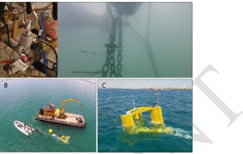
24
FIGURE 1
691
692
693
Figure 1. Deployment site adjacent to Faro-Olhão Inlet (A), the Faro Channel of Ria Formosa lagoon system
694
(Algarve, Portugal), where E1 Evopod (B) operated. The channel is generally oriented NW–SE, has a length of 9 695
km, and covers an area of 337 km2. The channel width is not constant, ranging from ~175 m to a maximum of
696
~625 m. The typical maximum depths along the channel range between 6 and 18 m (below mean sea level). 697
698 699
25
FIGURE 2
700
701
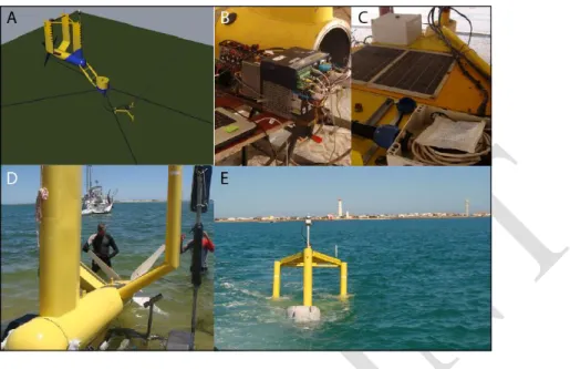
702
Figure 2. (A) Scheme of E1 with the mooring lines spreading from the mid-water buoy; (B) inside components
703
connect to the squirrel logger; (C) detail of the deck with the solar panels and control box; (D) E1 launch on the 704
water and (E) it trawl to the deployment site. 705
26
FIGURE 3
707
708
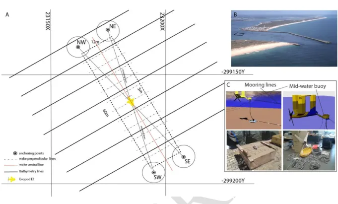
709
Figure 3. (A) Scheme of the deployment site, with the mooring locations and line spreading. Also represented are
710
the bathymetry lines 10 m spaced, the wake perpendicular lines and wake central line where bottom-tracking 711
ADCP and static measurements were performed, respectively; (B) Deployment area represented over an oblique 712
image of Faro-Olhão Inlet; (C) mooring scheme and material used on the deployment (e.g. anchoring weight, 713
chains, marking buoys, cable wire, etc). 714
27
FIGURE 4
716
717
718
Figure 4. (A) Detail of the load cells and its placing on the mooring lines; (B) Deployment day and boats used on
719
the mooring operation; (C) E1 deployed on 8th June 2017.
720 721 722
28
FIGURE 5
723
724
725
Figure 5. (A) Bathymetric survey using a RTK-DGPS synchronized with the single beam echo-sounder; (B)
726
Characterization of the 3D flow pattern using boat mounted (with bottom tracking) and bottom mounted ADCPs; 727
(C) Acoustic measurements with a hydrophone bottom mounted; and (D) ROV videos a for habitat 728
characterization. 729
730
29 FIGURE 6 732 733 734 735
Figure 6. Percent of time during a 14 period simulation with occurrence of tidal currents for the Faro-Olhão Inlet
736
area: A) with velocities stronger than 0.7 ms-1, and B) with velocities stronger than 0.7 ms-1 and lower than 1.75
737
ms-1.
738 739 740
30
FIGURE 7
741
742
743
Figure 7. Location of the ROV transects carried out in the survey areas during each tidal regime.
744 745
31
FIGURE 8
746 747
748
Figure 8. Side scan sonar mosaic of the study area.
749 750
32 FIGURE 9 751 752 753
Figure 9. Time-series of computed horizontal velocity magnitudes at each cell collected with the Nortek AS
754 Signature 1Mz. 755 756 757 758
33 FIGURE 10 759 760 761 762
Figure 10. (A) Peak ebb current velocities measured at E1 deployment site. Each profile corresponds to an
763
ensemble collected with the Sontek ADCP 1.5kHz with bottom tracking at a 5 s interval; (B) estimated electrical 764
power output for E1 based on the ADCP measurements for a flood-ebb spring-tide (red line). 765
766 767
34
FIGURE 11
768 769
770
Figure 11. Mean values (± standard deviation) of the percent-cover of Bugula neritina in both areas surveyed
771
during the study period. T-3: 3 days before to the deployment; T+ 8, T+15 and T+63: 8, 15 and 63 days after the 772
turbine had been installed. 773 774 775 0 5 10 15 20 25 30 35 T-3 T+8 T+15 T+63 P er ce nt -co v er ( %) CONTROL TURBINE
35
FIGURE 12
776 777
778
Figure 12. (A) Time-frequency analysis of the time series collected from 26th January to 1st of February 2017 by
779
means of an autonomous hydrophone mounted on a tripod (only the 2nd half is shown). The analysis has been
780
performed using observation windows of 4096 samples (≈ 0.077 s) which have been averaged to 90 s using the 781
Welch method; (B) Time-frequency analysis data collected at time 15:12 at 8th November 2017 by means of an 782
autonomous hydrophone operated from a boat. The analysis has been performed using observation windows of 783
16384 samples (≈ 0.311 s). 784
36
FIGURE 13
786
787
788
Figure 13. Time series of E1 parameters during a spring-neap tidal cycle. From top to bottom the panels present:
789
(i) drag forces recorded by the load cell; (ii) generated voltage; (iii) generated amperage; (iv) electrical output; (v) 790
current speed; (vi) raw power and (vii) E1 efficiency. 791
37 FIGURE 14 793 794 795 796 797
Figure 14. (A) Computed CT for both load cells placed at E1 moorings; (B) observed tension forces for both load
798
cells and fitted quadratic drag law. 799
800
801
802
38 FIGURE 15 804 805 806 807 808
Figure 15. (A) Comparison between E1’ electrical power curve and the observed electrical power outputs; (B)
809
Observed efficiencies, ηCP, of E1 at various flow speeds.
810 811