UNIVERSIDADE TÉCNICA DE LISBOA
INSTITUTO SUPERIOR DE ECONOMIA E GESTÃO
DOUTORAMENTO EM GESTÃO
NEUROSCIENCE IN MARKETING
AN FMRI-BASED PERSPECTIVE ON BRANDS
J
OSÉP
AULON
EVESC
ORREIAM
ARQUES DOSS
ANTOSOrientação: Doutor Luiz Abel Magro Moutinho
Júri:
Presidente: Reitor da Universidade Técnica de Lisboa
Vogais: Doutor Luiz Abel Magro Moutinho
Doutora Amanda Jayne Broderick
Doutora Maria Margarida de Melo Coelho Duarte
Doutor Paulo de Neville da Cunha Sepúlveda e Lencastre
Doutora Patrícia Margarida Piedade Figueiredo
ERRATUM
ABBREVIATIONS, UNITS AND ACRONYMS
AGL Artificial Grammar Learning AIC An information criterion (Akaike) ANN Artificial neural networks
aMPFC Anterior medial prefrontal cortex arMFC Anterior rostral medial frontal cortex
BC Before Christ
BOLD Blood-oxygen-level Dependent ca. Circa (Latin); approximately
cf. Confer (Latin); compare cont. Continued Coord. Coordinates
dMPFC Dorso medial prefrontal cortex
DN Default network
dof Degrees of freedom doi Digital object identifier
EPI Echo-planar imaging
ESRC Economic and Social Research Council et al. Et alii (Latin); and others
etc. Et cetera (Latin); and the rest
EV Explanatory variables
FEAT FMRIB Expert Analysis Tool
fMRI Functional Magnetic Resonance Imaging
FMRIB Functional Magnetic Resonance Imaging of the Brain
fNIRS-DOT Functional Near-Infrared Spectroscopy – Diffuse Optical Tomography fov Field of view
FSL FMRIB Software Library GLM General Linear Modelling HRF Hemodynamic response function
Hz Hertz (frequency; occurrences per second) IAPS International Affective Picture System
IC Independent component
IFG Inferior frontal gyrus IGT Iowa Gambling Task
IQR Interquartile range
ISI Inter-stimulus interval
MEG Magnetoencephalography
MELODIC Multivariate Exploratory Linear Optimized Decomposition into Independent Components
MNI152 Montreal Neurological Institute standard brain with 152 subjects
MO Market orientation
ms Milliseconds
MTL Medial temporal lobe
NBO Non-biological actors
oMFC Orbital medial frontal cortex
PAD Pleasure – Arousal – Dominance scale PCC Posterior cingulate cortex
PICA Probabilistic independent component analysis prMFC Posterior rostral medial frontal cortex
rTMS Repetitive Transcranial Magnetic Stimulation s Second
s/he She or he
SD Standard deviation
SI Primary somatosensory cortex SII Secondary somatosensory cortex
SAM Self-assessment manikin
S-O-R Stimulus – Organism – Response T Tesla
TE Echo time
TMS Transcranial Magnetic Stimulation ToM Theory of Mind
TPJ Temporo-parietal junction
TR Repetition time
ABSTRACT
Although somewhat outdated, the American Marketing Association definition of
brand still is largely accepted. In this case, brands are signs for product differentiation.
The present research, instead, finds brands and their logos as meaningful signs
that belong to the human communicative lexicon. Logos are ideograms, i.e. graphic
representations that convey meanings. These meanings are transferred from one mind to
other minds through brands, establishing communication between humans, and which is
also used to self-monitoring in a self-reflexive process, i.e., reading the reactions of
others to the ideographic messages once sent to them. Brands are intimately connected
to meta-representational processes, whether they are seen as the repository of human
attributes, whether themselves are perceived as interlocutors, in a quasi-human level.
It also finds that the human emotion system is used to perceive, interpret, and
classify brands. Founding in the neuro-based model of emotions developed by Damásio,
the present research reveals that brands systematically recruits the emotion system when
stimulate brains, which leads to posit that brands are felt in order to be perceived.
It is also largely relying in the brain structures that support emotion processing,
but also based in other regions that support self-relatedness processing, that is trained an
artificial neural network that yields predictions of subjects’ choices at a level much
higher than mere chance. This procedure allows a coarse but promising consumers’
“mind reading”.
RESUMO
Apesar de algo ultrapassada, a definição de marca da American Marketing
Association ainda é largamente aceite. Assim, as marcas são sinais usados na
diferenciação de produtos. A investigação presente, pelo contrário, sugere que as marcas
e os seus logótipos são sinais com significado que pertencem ao léxico comunicativo
humano. Os logótipos são ideogramas, i.e. representações gráficas que transmitem
significados. Tais significados transferem-se de uma mente para outra através das
marcas, estabelecendo uma comunicação entre humanos, e que também é usada na
auto-monitorização num processo auto-reflexivo, i.e. lendo as reacções que os outros têm às
mensagens ideográficas que lhes foram enviadas. As marcas estão intimamente ligadas
aos processos meta-representacionais, seja por elas serem consideradas um repositório
de atributos humanos, seja por elas próprias serem consideradas como interlocutores, a
um nível quase-humano.
Este estudo também constata que o sistema emocional humano é usado para
perceber, interpretar, e classificar as marcas. Baseado no modelo neuronal das emoções
de Damásio, verifica-se que as marcas recrutam sistematicamente o sistema das
emoções sempre que elas estimulam um cérebro, o que leva a avançar que as marcas são
sentidas de forma a serem percebidas.
É com base em estruturas cerebrais que sustentam o processamento das
emoções, mas também com base em outras regiões ligadas a processamentos da
auto-reflexão, que é treinada uma rede neuronal artificial, da qual resultam previsões das
escolhas dos sujeitos participantes, as quais estão a um nível muito superior ao mero
acaso. Este procedimento permite uma “leitura da mente” algo grosseira, mas muito
INDEX
Erratum ... 2
Abbreviations, Units and Acronyms ... 3
Abstract ... 5
Index ... 7
List of Tables ... 11
List of Figures ... 14
Preface ... 22
Original Contributions ... 23
Publications ... 24
Acknowledgments ... 26
I. Approaching the Theme, Bounding the Research, and Options ... 27
Neuroscience in Marketing ... 28
Functional Magnetic Resonance Imaging (fMRI) ... 31
FMRI basics. ... 32
General Linear Modelling (GLM) analysis of fMRI data. ... 36
Multivariate analysis of fMRI data. ... 42
Neuroscientific Approach to Brands ... 51
Three Principles from Grounded Theory ... 60
Peircean Semiotics on Brands Perception and Interpretation ... 64
Balancing between companies’ and consumers’ perspectives. ... 64
Brands’ syntax, signs, and memeplexes. ... 66
Brands and the Speculative Grammar: syntagmatatic semantics. ... 74
Brands as logical syntagmatatic entities (functions). ... 77
Aims ... 79
II. First Approach: A Study on Brands’ Implicit and Explicit Impressions... 82
Results ... 86
Behavioural results. ... 86
Activations produced in the brain that characterise the implicit paradigm (contrast
implicit > explicit). ... 88
Activations produced in the brain that characterise the explicit paradigm (contrast explicit > implicit). ... 88
Grounding Discussion ... 91
Digest and Introducing the Second Step ... 97
III. Second Step: Emotional and Social Relevant Contents in Different Categories of Brands ... 100
Results ... 100
Contrast positive > indifferent. ... 101
Conjunction between positive and indifferent valences. ... 103
Model-free analysis with MELODIC. ... 104
Grounded Discussion ... 107
Role of emotions in brands’ appraisal. ... 107
Brands’ symbolic meanings. ... 111
Digest, Some Limitations, and Introducing the Third Study ... 115
IV. Positive, Indifferent, and Fictitious Brands' Logos Perception: An Event-related fMRI Study ... 118
Results ... 120
Brands’ logos rating with the SAM in the PAD scale. ... 120
Consistency in the assessments between the sessions. ... 125
Response time. ... 128
Contrasting logos versus baselines. ... 130
Contrasting recognised brands versus fictitious logos. ... 144
Preferred brands versus the indifferent ones. ... 152
Indifferent and fictitious logos versus positive brands. ... 160
Multivariate independent components analysis. ... 164
Floating time window analysis of the vmPFC. ... 188
Grounding Discussion ... 199
Using the SAM and the PAD scale to assess brands... 199
Reaction time is enough to detach positive brands from the remaining. ... 202
Multi-baselines in fMRI experiments on brands. ... 203
Perceiving brands after logos perception. ... 217
Neural correlates of preferred brands. ... 222
The involvement of the ventro medial prefrontal cortex. ... 222
Investigating a possible influence of the Default Network. ... 231
Motor and somatosensory cortices. ... 233
The cluster marginal to the sylvian fissure. ... 234
Integrative overview of positive brands appraisal. ... 240
Investigating delayed decisions for indifferent and fictitious logos. ... 244
Imitation During Brands’ Appraisal ... 246
Syntactic roles assigned to the left inferior frontal gyrus... 246
The paradox. ... 246
Hypothesising the involvement of the mirror neurons system. ... 249
A multivariate analysis of the participation of the mirror neurons system. ... 250
Considerations about imitation and meaningful brands. ... 252
Digest, Some Limitations, and Introducing the Analysis with ANNs ... 255
V. S-O-R: Tackling the Psyche of the ‘O’ by Applying ANN ... 259
Data Pre-processing ... 259
Constructing the Artificial Neural Network ... 262
Interpretation of the Artificial Neural Network ... 262
Considerations about the Interpretation ... 268
Future Developments ... 269
VI. The Emergence of a Model ... 271
Symbolic Interactionism ... 271
Memetics and Imitation ... 273
Designing a Model ... 277
VII. Further Steps ... 281
How do Logos Convey Brands’ Experience? ... 281
Asocial Behaviour in Autism ... 282
Evolutionary Perspectives ... 286
Language and Writing... 290
Approaching Brands through Artificial Grammar Learning (AGL) ... 293
Experimental Design ... 297
Human Subjects ... 299
Data Acquisition ... 300
Image Analysis... 300
Appendix B Paradigm and Data Analysis in the Second Step ... 304
Paradigm ... 304
Image Analysis... 304
Appendix C Method in the Event-related fMRI study ... 307
Experimental Design ... 307
General structure. ... 307
Brands’ selection. ... 307
Fictitious logos. ... 309
Non-emotional words as second baseline. ... 309
Structuring the paradigm. ... 310
Instructions for the scanning session. ... 310
Human Subjects ... 312
Data Acquisition ... 312
Image Analysis... 313
General Linear Model analysis - common procedures... 313
General Linear Model analysis - conventional fixed time window analysis. ... 314
General Linear Model analysis - floating time window analysis. ... 315
General Linear Model analysis - group analysis. ... 316
Probabilistic Independent Component Analysis. ... 316
Identification of the anatomical brain structures. ... 317
Appendix D Paradigm Sequencing and Optimisation in the event-related fMRI study ... 319
LIST OF TABLES
Table 1 - Main independent components from MELODIC. ... 105
Table 2 - Votes on manikins or dots in the Pleasure and Arousal dimensions in the session previous to scanning, together with the respective z statistic (population proportion). ... 122
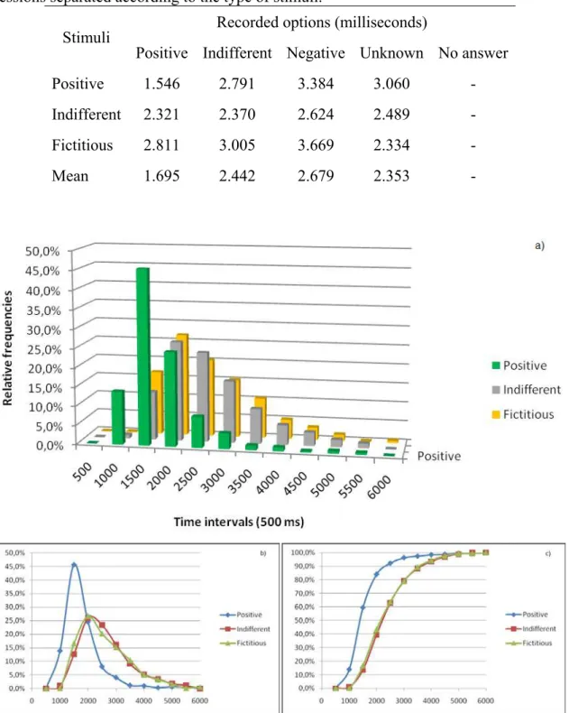
Table 3 - Assessments during the scanning sessions separated according to the type of stimuli. ... 125
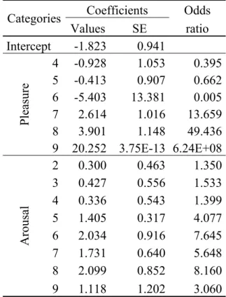
Table 4 - Coefficients of the multinomial logit model and the odds ratio for the
categories in the pleasure and arousal dimensions. ... 127
Table 5 - Confidence intervals at 95% level of the multinomial logit model for the categories in the pleasure and arousal dimensions. ... 127
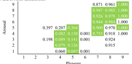
Table 6 - Predicted probabilities of the multinomial logit model for the categories in the
pleasure and arousal dimensions. ... 128
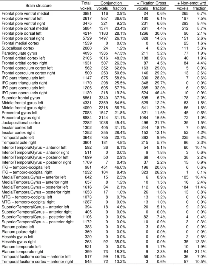
Table 7 - Mean reaction times in milliseconds of the assessments during the scanning sessions separated according to the type of stimuli. ... 129 Table 8 - Activated voxels (2 × 2 × 2 mm) for the contrasts between positive brands and
the baselines. Conjunction between the two contrasts, and voxels unique to each one. ... 134 Table 9 - Activated voxels (2 × 2 × 2 mm) for the contrasts between indifferent brands
and the baselines. Conjunction between the two contrasts, and voxels unique to each one. ... 136 Table 10 - Activated voxels (2 × 2 × 2 mm) for the contrasts between fictitious logos
and the baselines. Conjunction between the two contrasts, and voxels unique to each one. ... 138 Table 11 - Activated voxels (2 × 2 × 2 mm) for the conjunction among the contrasts
between all logos (positive, indifferent, and fictitious) and both baselines, and voxels unique to each one. ... 141 Table 12 - Activated voxels (2 × 2 × 2 mm) for the contrasts between positive and
indifferent brands vs. fictitious logos. Conjunction between the two contrasts, and voxels unique to each one. ... 145 Table 13 - Activated voxels (2 × 2 × 2 mm) for the contrasts between fictitious logos vs. positive and indifferent brands. Conjunction between the two contrasts, and voxels unique to each one. ... 148 Table 14 - Activated voxels (2 × 2 × 2 mm) for the contrast between positive versus
indifferent brands. ... 153
Table 16 - Activated voxels (2 × 2 × 2 mm) for the contrasts between positive vs. indifferent and fictitious logos. Conjunction between the two contrasts, and voxels unique to each one. ... 161
Table 17 - Selected z statistics that represent the fit between the contrasts of explanatory variables and the independent components calculated in the multivariate analysis, together with the F-test across subjects for each selected independent component. ... 165
Table 18 - Composition of the networks represented in independent components 18 and 41, which correlate with the process of brands recognition (voxels 2 × 2 × 2 mm). ... 166
Table 19 – Statistic z in independent components 18 and 41 from the multivariate analysis, of selected voxels from the GLM analysis. ... 169
Table 20 - Composition of the networks represented in independent component 22 which correlate with the process of brands preference (voxels 2 × 2 × 2 mm). ... 171 Table 21 - Composition of the networks represented in independent component 132
which correlate with the process of brands preference (voxels 2 × 2 × 2 mm). ... 173 Table 22 – Statistic z in independent components 22 and 132 from the multivariate
analysis, of selected voxels from the GLM analysis. ... 175
Table 23 - Composition of the networks represented in independent component 17 which correlate with the process of brands preference (voxels 2 × 2 × 2 mm). ... 177 Table 24 - Composition of the networks represented in independent component 27
which correlate with the process of brands preference (voxels 2 × 2 × 2 mm). ... 179 Table 25 – Statistic z in independent components 17, 27 and 118 from the multivariate
analysis, of selected voxels from the GLM analysis. ... 182
Table 26 - Composition of the networks represented in independent component 33 which correlate with the process of brands preference (voxels 2 × 2 × 2 mm). ... 184 Table 27 - Composition of the networks represented in independent component 36
which correlate with the process of brands preference (voxels 2 × 2 × 2 mm). ... 186 Table 28 – Statistic z in independent components 9 and 33 from the multivariate
analysis, of selected voxels from the GLM analysis. ... 188
Table 29 – Search in the output ICs for activations and deactivations in brain structures that compose the DN. ... 194
Table 30 - Selected z statistics that represent the fit between the contrasts of explanatory variables and the independent components calculated in the multivariate analysis, together with the F-test across subjects for independent components that have significant activated voxels within the brain structures that encompass the mirror neurons system. ... 251
Table 31 - Voxels selected for the artificial neural network inputs. ... 261
order), and random values from a uniform distribution (columns Random inputs). ... 262
Table 33 - Weights and bias that structure the neural network between the input and hidden layers. ... 264
Table 34 - Weights and bias that structure the neural network between the hidden and output layers. ... 264
LIST OF FIGURES
Figure 1 – Example of the BOLD signal output during fMRI experiments. The data used refers to 50 acquisitions, which in this case is 150 seconds. ... 35
Figure 2 – The orange line represents stimulus onsets and extinctions. The blue line is the resulting hemodynamic response function convolution, which already includes the delay in BOLD signal. ... 37
Figure 3 - Hemodynamic response function for two different stimuli. ... 37
Figure 4 - Hemodynamic response function for two different stimuli (blue and red lines) together with the BOLD signal for the voxel (-6 × 50 × -8) (green line). ... 38 Figure 5 - Hemodynamic response function for two different stimuli (blue and red lines) together with the BOLD signal for the voxel (-2 × 88 × -8) (yellow line). ... 38 Figure 6 - Hemodynamic response function for two different stimuli (blue and red lines) together with the BOLD signal for the voxel (-38 × 14 × -8) (grey line). ... 39 Figure 7 – Example of a statistical parametric map for the slice z = -08 (in this case, z is
the vertical axis of the coordinate system, not a statistical z). The points 1, 2, and 3 refer to the partial timecourses represented respectively in Figure 4, Figure 5, and Figure 6. The respective coordinates in the MNI152 coordinate system are: for point 1 (-6 × 50 × -8), for point 2 (-2 × -88 × -8), and for point 3 (-38 × 14 × -8). 40 Figure 8 – Example of the segmentation of the brain structures considered in the
adopted atlases in the slice z = -08. ... 41
Figure 9 - Example of the activations in Figure 7 (z = -08), now depicted in false
colours to highlight the participation of different brain structures. ... 41
Figure 10 - Example of the deactivations in Figure 7 (z = -08), now depicted in false colours to highlight the participation of different brain structures. ... 42
Figure 11 - An example of an artificial neural network architecture with n inputs, 3 nodes in the hidden layer, and 2 output nodes. ... 46
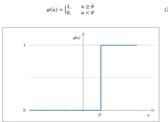
Figure 12 – Graphical representation of a step function like the one in Equation 2. ... 47
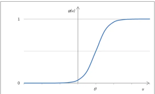
Figure 13 - Graphical representation of the sigmoid function like the one in Equation 3. ... 49
Figure 14 – The same ANN example from Figure 11, now emphasising the formative sector (in blue) and the reflective sector (in green). ... 49
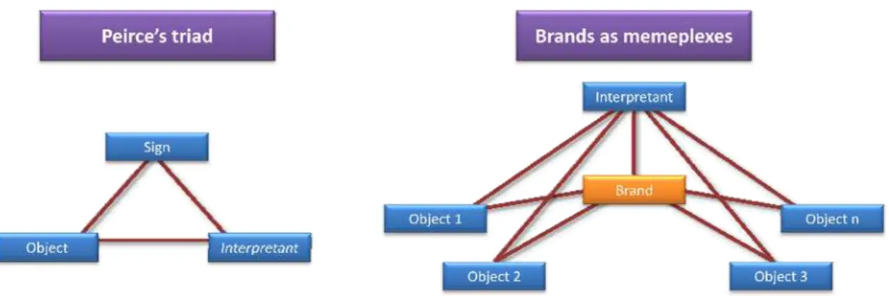
Figure 15 – Representing the memeplexic nature of brands using Peirce’s triad as a framing mould. ... 68
fusiform gyrus; FOC: frontal orbital cortex; Hip: hippocampus; mFP: medial frontal pole; pCG: paracingulate gyrus; MNI152 coordinates). ... 87
Figure 17 – Selected peristimulus hemodynamic response in two voxels: A (-08, 62, 30) that corresponds to the frontal pole (67%) in probabilistic atlases, and B (-06, 16, 44) that corresponds to the paracingulate gyrus (61%) in probabilistic atlases (MNI152 coordinates). ... 87
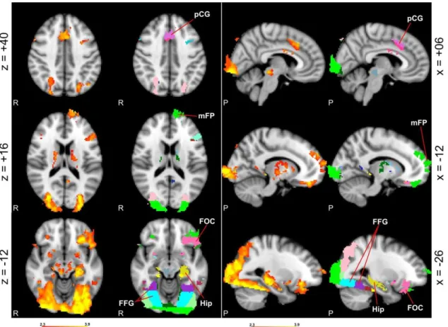
Figure 18 – Independent component (IC) 32 selected from the model-free analysis with MELODIC. This component explains 1.04% of the total variance. (a) The top row depicts thresholded activations and deactivations. The bottom row refers to only to the thresholded activations with brain structures highlighted in false colours (R: right; P: posterior; Amy: amygdala; FFG: fusiform gyrus; FMC: frontal medial cortex; FOC: frontal orbital cortex; FOp: frontal operculum cortex; Ins: insular cortex; mFP: medial frontal pole; pCG: paracingulate gyrus; MNI152 coordinates). (b) Timecourse of the IC 32 and full model fit; F-test on the full model fit: F = 686.01 (dof1 = 2; dof2 = 317) p < 0.00001; Contrast of parameter: z = 22.96; p < 0.00001. (c) Powerspectrum of the timecourse. The frequency of the peak is 1.67 Hz/100, which corresponds to a period of 60 seconds. ... 89
Figure 19 - Activations that characterise the implicit task when contrasted with the explicit (statistical parametric maps produced by FEAT). The left column refers to the thresholded map (z > 2.3), and the right column refers to the thresholded activations with the brain structures highlighted in false colours (R: right; P: posterior; Amy: amygdala; FMC: frontal medial cortex; pHG: parahippocampal gyrus; MNI152 coordinates). ... 90
Figure 20 - Activations that characterise the explicit task when contrasted with the implicit (statistical parametric maps produced by FEAT). The left column refers to the thresholded map (z > 2.3), and the right column refers to the thresholded activations with the brain structures highlighted in false colours (R: right; P: posterior; FOp: frontal operculum cortex; IFG: inferior frontal gyrus (comprising the pars opercularis and the pars triangularis); Ins: insular cortex; lFP: lateral frontal pole; Pal: pallidum; Put: putamen; MNI152 coordinates). ... 90
Figure 21 - Activations obtained contrasting the positive with the indifferent assessments in the axial (z = -12) and sagittal (x = -06) planes (statistical
parametric maps produced by FEAT). The first row refers to the thresholded map (z > 2.3), and the second row refers to the thresholded activations with the brain structures highlighted with false colours. (R = right; P = posterior; FMC – frontal medial cortex; mFP – frontal pole; PCG – paracingulate gyrus; MNI152
coordinates). ... 101
Figure 22 - Unthresholded z maps obtained with the contrast between the positive and indifferent assessments in the axial (z = -12, and +34) planes (statistical parametric maps produced by FEAT). The thresholded clusters (z > 2.3) are outlined in black. (R = right; vmPFC – ventro medial prefrontal cortex; dlPFC – dorso lateral
prefrontal cortex; MNI152 coordinates). ... 102
Figure 24 - FMRI maps for the conjunction analysis in the axial (z = -08, +04, and +36) and sagittal (x = -04) planes (statistical parametric maps produced by FEAT). The first row refers to the thresholded map (z > 2.3), and the second row refers to the thresholded activations with the brain structures highlighted with false colours. (R = right; P = posterior; aCG: anterior cingulate gyrus; aIns: anterior insular cortex; Cau: caudate; FObC: frontal orbital cortex; FOpC: frontal operculum cortex; Hip: Hippocampus; Pal: pallidum; PCG: paracingulate gyrus; PHG: parahippocampal gyrus; Put: putamen; MNI152 coordinates). ... 104
Figure 25 - The SAM - self-assessment manikin for pleasure and arousal dimensions used to assess brand's logos previously to the fMRI session. ... 121
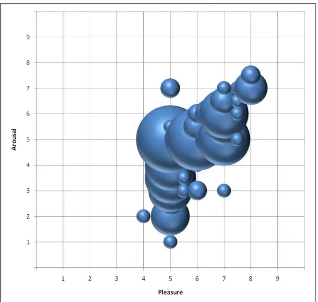
Figure 26 - Brands' logos votes obtained previously to the scanning session plotted in the Pleasure – Arousal matrix. The diameter of the circles is proportional to the quantity of votes. The green dashed rectangle bounds the criteria for positive brands selection, and the orange dashed line draw the limits for the criteria for the selected indifferent brands. ... 122
Figure 27 - Plot of the medians of brands' assessments in the Pleasure – Arousal matrix. The diameter of the circles is proportional to the quantity of votes. ... 123
Figure 28 - Plots of the votes of the two brands (F. C. Porto and S. L. Benfica) whose medians were Pleasure 5, Arousal 7. The diameter of the circles is proportional to the quantity of votes. ... 124
Figure 29 - Graphs with the relative frequencies of the response times obtained during the scanning session grouped in 500 ms intervals. Only the votes consistent
between the two sessions were considered. a) and b) ocurrences in the intervals; c) cumulative ocurrences. ... 129
Figure 30 - FMRI maps for the contrasts between positive rated brands and the baselines, and the respective conjunction analysis in the axial (z = -16, +04, and +28) and sagittal (x = -06, and -50) planes (statistical parametric maps produced by FEAT). The first and second rows refer to the thresholded maps (z > 2.3),
respectively, the contrast between positive versus fixation cross, and the contrast between positive and non-emotional words. The third row is the conjunction
analysis where common voxels are in green colour, voxels that activate only for the contrast positive versus fixation cross are in red, and voxels that activate only for the contrast positive versus non-emotional words are in blue. Radiological
convention; MNI152 coordinates. ... 131
Figure 31 - FMRI maps for the contrasts between indifferent rated brands and the baselines, and the respective conjunction analysis in the axial (z = -16, +04, and +28) and sagittal (x = -06, and -50) planes (statistical parametric maps produced by FEAT). The first and second rows refer to the thresholded maps (z > 2.3),
Figure 32 - FMRI maps for the contrasts between fictitious logos and the baselines, and the respective conjunction analysis in the axial (z = -16, +04, and +28) and sagittal (x = -06, and -50) planes (statistical parametric maps produced by FEAT). The first and second rows refer to the thresholded maps (z > 2.3), respectively, the contrast between fictitious logos versus fixation cross, and the contrast between fictitious logos and non-emotional words. The third row is the conjunction analysis where common voxels are in green colour, voxels that activate only for the contrast fictitious logos versus fixation cross are in red, and voxels that activate only for the contrast fictitious logos versus non-emotional words are in blue. Radiological convention; MNI152 coordinates. ... 133
Figure 33 - FMRI maps for the conjunction analysis among the contrasts between positive brands, indifferent brands, and fictitious logos and both baselines in the axial (z = -16, +04, and +28) and sagittal (x = -06, and -50) planes (statistical parametric maps produced by FEAT). The first row contains the conjunction maps where common voxels are in green colour, voxels that activate only for the
contrasts with the fixation cross are in red, and voxels that activate only for the contrasts with non-emotional words are in blue. The second row includes the maps with the conjunction analysis with the previous three types of voxels merged. In these maps the diverse brain structures are individualised with different colours. Radiological convention; MNI152 coordinates. ... 140
Figure 34 - Parameter estimates for positive, indifferent, and fictitious stimuli, and also for the non-emotional words (NEW) in two foci: the insular cortex, and the frontal orbital cortex. MNI152 coordinates. Error bars correspond to the confidence
intervals at 95%. ... 143
Figure 35 - Parameter estimates for positive, indifferent, and fictitious stimuli, and also for the fixation cross (Fix. Cross) in three foci of the paracingulate gyrus: dorsal, medial, and ventral. MNI152 coordinates. Error bars correspond to the confidence intervals at 95%. ... 144
Figure 36 - FMRI maps for the contrasts between real logos (positive and indifferent) versus fictitious logos, and the respective conjunction analysis in the axial (z = -16, +04, and +28) and sagittal (x = -06, and -50) planes (statistical parametric maps produced by FEAT). For each contrast the first row refers to the thresholded maps (z > 2.3), and in the second row the brain regions are individualised with different colours. In the conjunction analysis row common voxels are in green colour, voxels that activate only for the contrast positive versus fictitious logos are in blue, and voxels that activate only for the contrast indifferent versus fictitious logos are in red. Radiological convention; MNI152 coordinates. ... 147
Figure 38 - Parameter estimates for positive, indifferent, and fictitious stimuli, and also for the non-emotional words (NEW) in two foci in visual regions: the cuneal cortex, and the occipital fusiform gyrus. MNI152 coordinates. Error bars
correspond to the confidence intervals at 95%. ... 151
Figure 39 - Parameter estimates for positive, indifferent, and fictitious stimuli, and also for the non-emotional words (NEW) in four foci: the frontal pole, the angular gyrus, the precuneous cortex, and the posterior cingulate gyrus. MNI152
coordinates. Error bars correspond to the confidence intervals at 95%. ... 152
Figure 40 - FMRI maps for the contrasts between positive versus indifferent brands in the axial (z = -16, +04, and +28) and sagittal (x = -06, and -50) planes (statistical parametric maps produced by FEAT). The first row refers to the thresholded maps (z > 2.3), and in the second row the brain regions are individualised with different colours. Radiological convention; MNI152 coordinates. ... 155
Figure 41 - Parameter estimates for positive, indifferent, and fictitious stimuli, and also for the non-emotional words (NEW) in four foci in the ventro medial prefrontal cortex cluster: frontal pole, paracingulate gyrus, frontal medial cortex, and
subcallosal cortex. The graphs are over a sagittal picture showing the cluster at x = -04. The location of each of the four voxels was projected into this sagittal picture along de x axis. MNI152 coordinates. Error bars correspond to the confidence intervals at 95%. ... 157
Figure 42 - FMRI z statistic maps for the contrast between positive versus indifferent brands in the axial planes z = -10, and z = +32 (statistical parametric maps produced by FEAT). The thresholded significant clusters (z > 2.3 for activations and z < -2.3 for deactivations) are outlined in white. For z = -10 the considered ventro medial prefrontal cortex (ventral medial prefrontal cortex, frontal medial cortex, ventral paracingulate gyrus, and subcallosal cortex) is outlined in green, and for z = +32 the middle frontal gyrus is outlined in green. In two example foci (one for activation and the other for deactivation), the parameter estimates graphs for positive, indifferent, and fictitious stimuli, and also for the non-emotional words (NEW) are plotted. Error bars correspond to the confidence intervals at 95%; radiological convention; MNI152 coordinates. ... 158
Figure 43 - Parameter estimates for positive, indifferent, and fictitious stimuli, and also for the non-emotional words (NEW) in the six local maxima of the third cluster in the contrast between positive and indifferent brands. The graphs are over a sagittal picture showing the cluster at x = -42 and over an axial picture showing the cluster at z = +10. The location of each of the six voxels was projected into the sagittal picture along de x axis and into the axial picture along the z axis. Error bars correspond to the confidence intervals at 95%; radiological convention; MNI152 coordinates. ... 159
Figure 44 - Parameter estimates for positive, indifferent, and fictitious stimuli, and also for the non-emotional words (NEW) in two foci of the forth cluster in the contrast between positive and indifferent brands: the insular cortex, and the central
Figure 45 - FMRI maps for the contrasts between indifferent and fictitious logos versus positive brands, and the respective conjunction analysis in the axial (z = -16, +04, and +28) and sagittal (x = -06, and -50) planes (statistical parametric maps
produced by FEAT). For each contrast the first row refers to the thresholded maps (z > 2.3), and in the second row the brain regions are individualised with different colours. In the conjunction analysis row, common voxels are in green colour, voxels that activate only for the contrast indifferent versus positive brands are in red, and voxels that activate only for the contrast fictitious logos versus positive brands are in blue. Radiological convention; MNI152 coordinates ... 163
Figure 46 - Independent components 18 and 41 fMRI maps for the multivariate analysis in the axial (z = -16, +04, and +28) and sagittal (x = -06, and -50) planes (statistical parametric maps produced by MELODIC). The brain regions are individualised with different colours. Radiological convention; MNI152 coordinates. ... 168
Figure 47 - Independent components 22 and 132 fMRI maps for the multivariate analysis in the axial (z = -16, +04, and +28) and sagittal (x = -06, and -50) planes (statistical parametric maps produced by MELODIC). For each independent component, top row depicts z statistics (activations and deactivations) and the bottom row depicts the same brain regions but individualised with different
colours. Radiological convention; MNI152 coordinates. ... 170
Figure 48 - Independent components 17 and 27 fMRI maps for the multivariate analysis in the axial (z = +16, +38, and +58) and sagittal (x = -06, and -50) planes
(statistical parametric maps produced by MELODIC). For each independent component, top row depicts z statistics (activations and deactivations) and the bottom row depicts the same brain regions but individualised with different
colours. Radiological convention; MNI152 coordinates. ... 176
Figure 49 - Independent components 33 and 36 fMRI maps for the multivariate analysis in the axial (z = -16, +04, and +28) and sagittal (x = -06, and -50) planes (statistical parametric maps produced by MELODIC). For each independent component, top row depicts z statistics (activations and deactivations) and the bottom row depicts the same brain regions but individualised with different colours. Radiological convention; MNI152 coordinates. ... 183
Figure 50 - Parameter estimates for the stimuli in the same four local maxima as in Figure 41. The baseline for comparison is the fixation cross. The bar graphs identified with the suffix (6s) are the conventional GLM-based analysis of fMRI data as in Figure 41. The bar graphs identified with the suffix (b) refer to the participation of the voxel before the decision instant (i.e. before button pressing). The bar graphs identified with the suffix (a) refer to the participation after the decision instant but before the stimulus offset MNI152 coordinates. Error bars correspond to the confidence intervals at 95%. ... 189
Figure 52 - Parameter estimates for the stimuli in the default network hubs (aMPFC and PCC) proposed by Andrews-Hanna et al. (2010). The baseline for comparison is the fixation cross. The bar graphs identified with the suffix (6s) are the
conventional GLM-based analysis of fMRI data. The bar graphs identified with the suffix (b) refer to the participation of the voxel before the decision instant (i.e. before button pressing). The bar graphs identified with the suffix (a) refer to the participation after the decision instant but before the stimulus offset MNI152 coordinates. Error bars correspond to the confidence intervals at 95%. ... 191
Figure 53 - Parameter estimates for the stimuli in the default network dMPFC
subsystem proposed by Andrews-Hanna et al. (2010). The baseline for comparison is the fixation cross. The bar graphs identified with the suffix (6s) are the
conventional GLM-based analysis of fMRI data. The bar graphs identified with the suffix (b) refer to the participation of the voxel before the decision instant (i.e. before button pressing). The bar graphs identified with the suffix (a) refer to the participation after the decision instant but before the stimulus offset MNI152 coordinates. Error bars correspond to the confidence intervals at 95%. ... 192
Figure 54 - Parameter estimates for the stimuli in the default network MTL subsystem proposed by Andrews-Hanna et al. (2010). The baseline for comparison is the fixation cross. The bar graphs identified with the suffix (6s) are the conventional GLM-based analysis of fMRI data. The bar graphs identified with the suffix (b) refer to the participation of the voxel before the decision instant (i.e. before button pressing). The bar graphs identified with the suffix (a) refer to the participation after the decision instant but before the stimulus offset MNI152 coordinates. Error bars correspond to the confidence intervals at 95%. ... 193
Figure 55 – Parameter estimates of the GLM fit for the 25 EVs with the timecourses for ICs 24 and 41. The comparison category is the baseline fixation cross. ... 198
Figure 56 - Parameter estimates for positive, indifferent, and fictitious stimuli, and also for the non-emotional words (NEW) in three foci in the left inferior frontal gyrus (IFG). MNI152 coordinates. Error bars correspond to the confidence intervals at 95%. ... 248
Figure 57 - Independent components 18, 41, and 100 fMRI maps for the multivariate analysis in the axial (z = -52) plane (statistical parametric maps produced by MELODIC). For each independent component, top row depicts z statistics and the bottom row depicts the same brain regions but individualised with different colours. In the right column there is a plane with the complete regions that belong to the mirror neurons system which serves as a key to interpret the planes on the left side: AnG - angular gyrus; aSMG - anterior supramarginal gyrus; pMTG - posterior middle temporal gyrus; POp - pars opercularis; pSMG - posterior supramarginal gyrus; pSTG - posterior superior temporal gyrus; PTr - pars
triangularis. Radiological convention; MNI152 coordinates. ... 251
3 (red colour) the second, third, and forth volumes after stimulus onset are
averaged. ... 260
Figure 59 - The transient model that emerged from the findings of this research, as well the investigations of several authors, in a form of an endless ring. The self-concept is at the centre, and eight linked satellites gravitate around. A brand is the idea that links all these concepts and each individual’s self-concept. ... 279
Figure 60 - Complete sequence of the trial. Duration is approximate. ... 297
Figure 61 - Schemas of the first four cycles (baseline / stimulus) for the assessments of the first two participants. Each stimulus block had five brands either rated as
positive, indifferent, or negative. These assessments were then used for event-related analysis. ... 304
PREFACE
Qualitative and Quantitative methods are not usually seen together in the same
research. Social Sciences and Natural Sciences (or Exact) tend to mutually repel, each
one with its credos and rituals. Compartmentalising knowledge only results in creating
difficulties to its progress. The approach of the present thesis is markedly no-dogmatic
and shamelessly incorporates methods and knowledge from both sides. Ultimately, its
aim is to know more about humans.
As it will emerge along the dissertation, brands are inherently and intrinsically
human. The last two decades witnessed the emergence of human facets in brands in a
series of ideographic studies. In fact, brands were not created two centuries ago and
brands are not only product differentiators. Such a way of thinking is clearly limited,
amputating brands in the most they are. Brands are crucial for self construction,
maintenance, and repairing. Brands are also used to mark belongingness to social
groups and avoidance too. Brands are used also to self-monitoring in a self-reflexive
process. Hence, brands are vital for psychosocial homeostasis, a concept with 40 years
that here is recovered and that wisely translates what brands are in fact.
Probably brands are as old as writing is. Brands belong to the human
communicational system. When the Native American paints his totem in the shield, he
is spreading his brand, sending clear messages with meanings about himself: what he is
and what he is not. Very importantly, he would not be the same without such brand.
Brands are not a western creation. It may be advanced that:
“27 So Man created brand in his own image, in the image of Man he created him;”
Original Contributions
The main original contributions of this research are:
A different framework to understand what brands are in fact. There is an
alteration from the traditional American Marketing Association definition,
which conceive brands as product markers, allowing to make a distinction from
the competing products, to the proposed framework, where brands belong to
the human communicative lexicon, much like in logographic / ideographic
language systems, and which integrates the Semiotic perspective that brands
(Signs) are different because convey different meanings (Objects).
It is revealed that the human emotion processing neural mechanism is largely
used to perceive and classify brands. In fact, brands are felt in order to be
perceived.
There is a significant participation of the Social Brain when brands’ logos
stimulate the brain. There is a consistent participation of brain structures
connected to Theory of Mind, which is interpreted as a “doing mind” with
brands, whether brands are perceived as repository of other humans attitudes
(humans mediators), whether brands are themselves the target of
meta-representations, in this case are brought into a quasi-human level.
Qualitative research in general and Grounded Theory in particular are not
usually seen in traditional positivist realms, like Neuroscience is. Grounded
Theory is a master girder along this research in a markedly post-positivist
approach. The compelling pertinence in theory construction, the systematic
empiric data bring robustness and purpose to any research, which counteracts
the insistence on narrowing questions into an atomic and meaningless level.
It is experimented a new approach to interpret MELODIC independent
components (ICs) outputs by the means of a GLM. The GLM links ICs to the
paradigms’ manipulations through the conventional explanatory variables
(EVs). This strategy allows selecting specific ICs with statistical criteria (and
not based in the suppositions of the researcher) and makes the usually large
output sets much easier to analyse and interpret.
It is experimented the application of artificial neural networks (ANNs) to the
analysis of Functional Magnetic Resonance Imaging (fMRI) data, developing
an initial procedure. This procedure is found to yield predictions of subjects’
options much higher than the chance level, allowing to a coarse but promising
“mind reading”.
Publications
Parts of this thesis have been presented and published in several scientific
conferences with competing papers:
Santos, José Paulo; Brandão, Sofia; Seixas, Daniela (2007). “Neuromarketing:
valence assessments of commercial brands. A functional magnetic resonance
imaging (fMRI) study”, 9th International Forum on the Sciences, Techniques
and Art Applied to Marketing. Academy and Profession (November 29-30th,
2007), at Universidad Complutense de Madrid, Spain.
Santos, José Paulo; Brandão, Sofia; Seixas, Daniela (2008). “Neuromarketing:
commercial brands”, XVIII Luso-Spanish Conference on Management
(February, 07-08th, 2008), at the Faculty of Economics of University of Porto,
Portugal.
Santos, José Paulo; Brandão, Sofia; Seixas, Daniela; Moutinho, Luiz (2008).
“Neural Correlates of Emotional and Symbolic Brands’ Content”, 2008
Conference on Neuroeconomics (May, 15-16th, 2008), at the Copenhagen
Business School, Copenhagen, Denmark.
Santos, José Paulo; Brandão, Sofia; Seixas, Daniela; Moutinho, Luiz (2009).
“Habeo ergo sum: neural correlates for self-concept nourishing with brands’
symbolic meanings”, 38th EMAC Conference (May 26-29th, 2009), at Audencia
– École de Management, Nantes, France.
Santos, José Paulo; Moutinho, Luiz; Seixas, Daniela; Brandão, Sofia (2010).
“Perceiving brands after logos perception: an event-related fMRI study”, 6th
Thought Leaders International Conference on Brand Management (April
ACKNOWLEDGMENTS
To José Diogo, José Guilherme and Cláudia Sofia, and of course José Queiroz
and Maria Ermelinda, for love, care, support, kept the universe stable and a truly
deadline.
But I am just one in the team: to Daniela Seixas, Sofia Brandão, and Luiz
I. APPROACHING THE THEME, BOUNDING THE RESEARCH, AND
OPTIONS
The 2008 call from the Economic and Social Research Council (ESRC)
“Understanding Individual Behaviour: Exploratory Networks (UIBEN)” summarises the
actual level of comprehension of human behaviour:
The ESRC in collaboration with the BBSRC and MRC invites applications for
innovative exploratory networks (ENs) in the area of 'Understanding Individual
Behaviour' (UIB). Many of the major challenges facing UK society depend on
improving understanding on why people behave as they do and how to maximise
the effectiveness with which individuals can take control of their own lives. The
leading edge is to bring together the different groups of scientists from very
different perspectives into a meaningful scientific endeavour which adds value
via its interdisciplinary approach. The complexity of analysing human
behaviour, as well as the challenges of cross-disciplinary working, both within
and between the biological, physical, biomedical and social sciences, means
achieving this aim will be especially demanding. (ESRC, 2008, retrieved
2008-08-07 http://www.esrc.ac.uk/ESRCInfoCentre/opportunities/current_funding_
opportunities/UIB.aspx?ComponentId=26866&SourcePageId=5964)
In fact the mechanisms and computations that output human behaviour still are a
mystery, and this state of the art directly touches Marketing discipline because
Markets are a human creation where individuals practise exchange and exchange is a
cascade of behavioural initiatives and responses. It is worth to note that the ESRC call
requires the participation of scientists from diverse fields to embark upon a new
multidisciplinary approach. It recognises the complexity of human, and consequently,
consumer, behaviour, and it is possible to infer that the conventional approaches were
not sufficient. It is time to involve Biology, Physics, and Biomedicine together with
Social Sciences to struggle to better understand human behaviour. The present work
shares the concern of ESRC and clearly adopts the proposed strategy.
Neuroscience in Marketing
The use of neuroscientific knowledge to investigate Marketing issues has been
postulated by several researchers and practitioners (Ambler, 2008; Hubert & Kenning,
2008; N. Lee, Broderick, & Chamberlain, 2007; D. Penn, 2008; Plassmann, Ambler,
Braeutigam, & Kenning, 2007; Zaltman, 2003). Even recently such visions were
disclosed in an high impact journal (Ariely & Berns, 2010). In spite of this, not many
empirical articles have been published in peer reviewed journals, contrarily to the
flourishing field of Neuroeconomics that already have a society (The Society for
NeuroEconomics; http://www.neuroeconomics.org), a scientific annual meeting, and
substantial articles and books (Glimcher, 2003; Glimcher, Camerer, Fehr, & Poldrack,
2009; Politser, 2008). Aiming to contribute with cutting-edge research to Neuroscience
applied to Marketing, the main object of the research along this work will be
commercial brands, represented by their logos, to target a neuroscientific approach to
But, why so big expectancies rely on Neuroscience? Maybe because actual
methods are not providing satisfactory answers... (Senior, Smyth, Cooke, Shaw, & Peel,
2007). Although the evolution in statistical analysis, much of the market research still
extensively depends on consumers opinions. It is known that humans give socially
desirable responses (Steenkamp, de Jong, & Baumgartner, 2010; Tourangeau & Yan,
2007), especially when the questions investigate delicate themes like drugs (Makkai &
McAllister, 1992), or emotions (Chamberlain & Broderick, 2007). In the end, the
researcher is working more with pretence than reality, more with papers that actors
would like to perform than those they effectively can or are able to perform. If the study
is contaminated with such biases, its utility and applicability will become very limited.
Acknowledging this problem, some researchers developed other methods that could
surpass this bias by limiting verbalisations, like the image-based in-depth personal
interview that Zaltman (2003) patented under the name ZMET - Zaltman Metaphor
Elicitation Technique (Zaltman, 1995). For example, this method was used to
understand the perceptions that consumers have about advertising (Coulter, Zaltman, &
Coulter, 2001), and the results obtained with the characterisation of mountain bike
consumers are strikingly pertinent, drawing a cognitive map that undresses this
consumer tribe (Christensen & Olson, 2002). However, consumers’ brains, particularly
the cognitive processes that occur in the brain and generate behaviours, still are a black
box. The faith on Neuroscience is that it would help shed some light into that black box,
and thus helps researchers and marketers to better understand consumers.
The following study conducted by Plassmann and colleagues may illustrate how
neuroscientific knowledge can inform about specific marketing issues (Plassmann,
Magnetic Resonance Imaging (fMRI) device while they tasted a set of wines and rated
them on pleasantness. The only things they knew about the wines were the grapes they
were made from (all Cabernet Sauvignon), and their prices. In fact, the task was being
manipulated because the researchers did not delivered five different wines (as
consumers thought), but only three. In two of them the price was increased / decreased.
Wine 1 was delivered at its market price ($5), and inflated ($45), wine 2 was delivered
at its market price ($90), and deflated ($10), and wine 3 was delivered at its market
price ($35). The ratings exhibited a clear linear correlation with price. Eight weeks after
the scanning session, participants had to rate again the wines, now without the price
information. They could not significantly distinguish wine 1 at $5 from $45, neither
wine 2 at $90 and $10. Amazingly, wine 1 ($5 and $45, but participants did not know
the price now) was the higher rated. This inverse correlation between price and wine
liking is confirmed in blind tests made with non-experts (Goldstein, et al., 2008). The
positive correlation between price and quality is known for long (Rao & Monroe, 1989),
and participants produced behavioural responses that were culturally aligned. The
comparison between high priced wines (wine 1 at $45, and wine 2 at $90) versus low
priced wines (wine 1 at $5, and wine 2 at $10) revealed activation in a brain region
named ventro medial prefrontal cortex and a deactivation in the dorso lateral prefrontal
cortex. This pattern suggests that the participants’ decision processes were
emotion-based and that they forwent their rational capabilities. In fact, participants were common
wine appreciators, not professionals. Thus, they did not use the necessary deliberative
knowledge to independently rate the wines, and hence, they used their emotional
cognition. It is worth to say that the experienced pleasantness price-based did not
responding according to some information other than the sensorial. For Marketing, this
is a clear lesson that intrinsic qualities of a product can be perfectly negligible, and
extrinsic properties, like price, can override functionalities during the decision process.
In fact, Neuroscience acknowledges that people have extreme difficulties in
representing absolute values. Common judgements are relative-valued, which turns
them permeable to manipulations as the described in this study, when the brain tries to
integrate several sources of information under uncertainty and produce accordingly
behaviours (Seymour & McClure, 2008).
In summary, the neuroscientific knowledge and methods can and should be used
to aid researchers understand better how consumers behave, and specifically how
consumers relate to brands (Perrachione & Perrachione, 2008). To this same conclusion
arrived Chamberlain and Broderick (2007), stressing that physiological measures concur
to a better description of a construct so complex as emotions are. This strategy is then
fully in line with the proposals and aims of ESRC considered in the beginning of this
chapter.
Functional Magnetic Resonance Imaging (fMRI)
Many neuroscientific studies have been using Functional Magnetic Resonance
Imaging (fMRI) to investigate brain function, and it was found to be useful in market
research (Kenning, Plassmann, & Ahlert, 2007). This Neuroimaging technique was
elected due to a set of advantages, where being ethically acceptable apply it to healthy
participants figures on the top (Seixas & Ayres Basto, 2008): it does not uses
radioactive chemicals, nor ionizing radiation, nor has the invasiveness of introducing
electromagnetic pulses that never have been proved to cause harm to humans. Other
advantages include the spatial resolution and a wealth of knowledge constructed along
the years of neuropsychological studies using fMRI, which is crucial to guarantee the
nomological validity of eventual findings. A set of disadvantages are important to be
mentioned to fully understand the outputs of this tool. The most important is the fact
that the fMRI scanner is located inside a hospital, which means that healthy participants
will perform in the trials under the hospital environment. The extent of the influence of
such environment is unknown, notwithstanding the adoption of practices that aim to
reduce such an influence like the use of current wearing apparel by team elements and a
fifteen minutes lounge talk, previous to the scanning sections, to ensure anxiety
reduction. It is worth to say that not all participants are acceptable in the experiments:
due to impositions of the Ethics Committee only adults are allowed to the scanner; due
to fMRI’s limitations, participants should not suffer from claustrophobia, nor have
metal particles in the body; and due to neuroscientific considerations, they should not be
under the effect of psychotropic drugs, nor be left handed (to guarantee the same brain
lateralisation for all participants). Other major disadvantages of fMRI are the noise
(intrinsic to the fMRI scanner operation) and the very limited interaction with
participants. These disadvantages limit the use of sound, touch, taste, and smell stimuli.
For that reason only visual stimuli will be used.
FMRI basics.
Some basics of fMRI should be considered to fully interpret and understand the
results (some books make a very complete draw of this tool (Huettel, Song, &
McCarthy, 2004; Jezzard, Matthews, & Smith, 2001), and Blow (2009) updates with the
signal). Thus, it does not measures directly neural activity but, supposedly, the rate of
oxygen consumption: it is assumed that when a group of neurons increase firing rate,
they start to consume more oxygen. Oxygen is supplied by the blood stream, linked to
haemoglobin molecule. Deoxihaemoglobin (haemoglobin without oxygen) is
paramagnetic (is attracted to magnetic fields), but oxyhaemoglobin is diamagnetic
(creates a magnetic field opposed to an external magnetic field), which means that,
when oxyhaemoglobin delivers the oxygen molecule that is carrying, it transforms into
deoxihaemoglobin and simultaneously changes its magnetic character. This change
interferes with magnetic field, and this interference can be measured by radiofrequency
pulses in three dimensional volumes.
As there is a difference in time between the neurons firing rate increase and the
extra supply of oxygen, the BOLD signal is lagged, and usually the peak occurs about 4
to 6 seconds after the stimulus onset. This feature is very important when interpreting
the results.
It results from this mechanism that if researchers aim to test if a certain group of
neurons participate in a process, they must design a paradigm that puts those neurons
into, at least, two different firing rates. This is a very important methodological issue, as
it results that only relative questions can be addressed with this tool. If this contrast
between two different levels does not exist there will only exist a constant firing pattern
in time, impossible to resolve with fMRI. In simple block designs, two levels of
functioning are usually induced by the paradigm: stimulus and baseline. More complex
paradigms use several classes of stimulus and a baseline, hoping that certain brain
structures fire differently under each different stimulus. By subtracting pairs (stimulus 1
the result is positive, which means that the target neurons increased the firing rate with
the stimulus onset; or a deactivation (increase in BOLD signal under the baseline
condition) if the result is negative, although this mechanism is not completely
understood (Logothetis, 2008; Wade, 2002). More complex analysis allows the
emergence of linear, parabolic, exponential, logarithmic, etc. parametric tendencies in
multi stimuli paradigms.
It is worth to emphasise that activation / deactivation and excitatory / inhibitory
impulses are not the same thing, although all concern neurons. So a neuron fire, it needs
to receive excitatory impulses from other neurons over a certain threshold. However,
some neurons send inhibitory impulses that counteract the excitatory ones, blocking the
excitatory chain. It is important to retain that if a neuron sends an excitatory impulse, or
if another one sends an inhibitory impulse, both are working, both are firing, thus both
are consuming more oxygen, and then both increase the BOLD signal. This means that
both excitatory and inhibitory neurons produce activations in the fMRI outputs (Sotero
& Trujillo-Barreto, 2007).
There are two more limitations of fMRI that extensively condition the design of
the research paradigms. Normally a full brain scan takes 2 to 3 seconds to accomplish.
Within this time window multiple processes initiate, evolve, and terminate. Hence,
fMRI is good to reveal the brain structures that participate in a process, but, actually, it
is not capable to disclose sequences within psychological processes. Another point is
that BOLD signal is laden with magnetic noise (an example of the output signal is
drawn in Figure 1). For this reason it is necessary to repeat enough times the same
stimulus and baseline so the signal statistically emerges from noise. Murphy and
Balancing all these pros and cons, the result is clearly positive for fMRI and this
technique was chose to address a specific Marketing issue: how humans perceive
brands. One of the aims of this thesis is to draw cognitive maps of assorted brands’
perception with the help of fMRI. This perception will be made up by consumers.
Hence, it will be the images of the brands, as consumers construct them in their brains,
which will be acquired. This research stresses therefore the shift into the consumer
perspective on brands, as consumers own the epicentre of equity building along their
relation with brands (Escalas, 2004; Keller, 1993; Lassar, Mittal, & Sharma, 1995;
Leone, et al., 2006). Based upon the activated brain structures it is intended to identify
the processes that support brands’ perception and infer the characteristic brands’
dimensions. The purpose of the present research is not study a particular brand, rather
find eventual neural markers that could be used to attribute certain characteristics to
brands, but with neuroscientific validity, hence surpassing the verbalisation pertained to
conventional methods like questionnaires, focus groups, or interviews.
General Linear Modelling (GLM) analysis of fMRI data.
The scanner outputs a dataset with the BOLD signal along the sequence of brain
acquisitions (let say “photos” in timely sequence). However, this timecourse is not for
all the brain. The brain is divided in voxels (think about voxels like digital photos’
pixels, but with thickness). If the unit voxel is 2 mm × 2 mm × 2 mm, it would expect to
have about 200,000 voxels in the whole brain (which is about 1,600 m3).
As the paradigm is manipulated and stimuli onset and duration is controlled, the
idea is to, for each voxel at a time, consider every type of stimulus an independent
variable, the BOLD signal is the dependent variable and then fit a GLM. Likewise, it is
possible to make statistical inferences over the independent variables’ coefficients (β,
betas) and then conclude about an eventual activation, or deactivation, or no significant
difference in the contrast. An example illustrates the procedure.
The orange line in Figure 2 represents the stimulus manipulation with the
respective onsets and extinctions. However, the BOLD signal is lagged about 4-6
seconds and also the hemodynamic response does not happen in right angles, but is
smooth. The first step is then to transform onsets and extinctions in a hemodynamic
Figure 2 – The orange line represents stimulus onsets and extinctions. The blue line is the resulting hemodynamic response function convolution, which already includes the delay in BOLD signal.
This procedure has to be extended to all independent variables. In Figure 3, the
HRF for two different stimuli are represented.
Figure 3 - Hemodynamic response function for two different stimuli.
The BOLD signal (dependent variable) may now be added to the graph (see
Figure 4. It is possible to see that the BOLD signal line follows more the blue line than
the red line. In fact the statistical z for this difference is 3.94. At this point it is necessary
to define a threshold for significance. The value arbitrated is the default in the FSL
software package: 2.30 for activations, and -2.30 for deactivations. As 3.94 > 2.30 it
Figure 4 - Hemodynamic response function for two different stimuli (blue and red lines) together with the BOLD signal for the voxel (-6 × 50 × -8) (green line).
In Figure 5 there is a different example for another voxel. In this case the yellow
line follows less the blue line than the red line. The statistical z for such difference is
-4.43, and as it is inferior to the threshold (-2.30) it may be asserted that this voxel
deactivates in the contrast Blue > Red.
Figure 5 - Hemodynamic response function for two different stimuli (blue and red lines) together with the BOLD signal for the voxel (-2 × 88 × -8) (yellow line).
A further example is presented in Figure 6. In this case the BOLD curve does
not follow preferentially any of the others, and the statistical z is -0.22. This voxel is not
Figure 6 - Hemodynamic response function for two different stimuli (blue and red lines) together with the BOLD signal for the voxel (-38 × 14 × -8) (grey line).
After running this procedure for all the voxels in the brain, the output is a
statistical parametric map with z values. This is why this kind of approach is named by
mass-univariate analysis: a GLM analysis is applied in each voxel per se; interactions
between voxels are not considered. To better visualise the relevant information, it is a
common procedure to highlight activated voxels with colours ranging from red to
yellow (normally corresponding to z from 2.30 to 3.90), and highlight deactivated
voxels with colours from dark blue to light blue (normally corresponding to z from
-2.30 to -3.90). Non significant voxels are not represented. To easily locate the voxels
exhibiting activations or deactivations, usually these colour codes are presented over an
anatomical acquisition of the brain, as depicted in Figure 7. Along the present work the
brain coordinate system and the brain template that will always be used as reference is
the MNI152, adopted by the International Consortium for Brain Mapping (details of the
construction of this coordinate system and brain template can be found in Collins (1994)
Figure 7 – Example of a statistical parametric map for the slice z = -08 (in this case, z is the vertical axis of the coordinate system, not a statistical z). The points 1, 2, and 3 refer to the partial timecourses represented respectively in Figure 4, Figure 5, and Figure 6. The respective coordinates in the MNI152 coordinate system are: for point 1 (-6 × 50 × -8), for point 2 (-2 × -88 × -8), and for point 3 (-38 × 14 × -8).
The identification of the anatomical brain structures that include the activated or
deactivated voxels is made with the help of digital atlases. Along the present work two
probabilistic atlases will be used: the Harvard-Oxford Cortical Structural Atlas and the
Harvard-Oxford Subcortical Structural Atlas provided by the Harvard Centre for
Morphometric Analysis (www.cma.mgh.harvard.edu), which are part of FSL View
v3.0.2, part of FSL 4.1.2. Maintaining the same slice example (z = -08), Figure 8
provides an image of the segmentation of these atlases; neighbouring brain structures
Figure 8 – Example of the segmentation of the brain structures considered in the adopted atlases in the slice z = -08.
It is possible then to filter the results of the activations / deactivations with these
atlases to conclude about the brain structures that participate in each process. The same
previous example is depicted in Figure 9 for the clusters with activations and in Figure
10 for deactivations.
Figure 10 - Example of the deactivations in Figure 7 (z = -08), now depicted in false colours to highlight the participation of different brain structures.
An important issue in using brain templates and standard brains is their
usefulness in group analysis. The procedure described so far applies for the analysis at
the individual level, which may be interesting for Psychology. However, for Marketing,
the most appealing are collective movements, which mean that the systematic search of
patterns of activation across individuals is emphasised. Due to inter-individual
morphological variations, comparing brains is a challenging task, and resorting to
standard brains is a suitable solution, acknowledging that in the adaptation process
valuable information will be lost and that such process is always approximate.
Multivariate analysis of fMRI data.
The analysis in a voxel by voxel basis puts methodological problems.
Acknowledging that fMRI is being used to unveil neural systems that support
psychological processes, the separate analysis of each element without considering the
effect of the remaining will ever be successful? Probably not, because the advantage of
a system is being more than the sum of the parts, and if psychological processes rely on
into the decision process), this strategy for data analysis maybe will never accomplish
its objective.
It has been proposed multivariate methods to analyse fMRI data (Haynes &
Rees, 2006; Norman, Polyn, Detre, & Haxby, 2006; Pereira, Mitchell, & Botvinick,
2009), which consider not only the timecourse signal of each voxel individually, but
also the activity in the other voxels through the brain. Of course this introduces
extensive amounts of computations, which is not easily solved. Due to this reason, most
of the multivariate approaches have been focusing on well defined parts of the brain
(regions of interest) and there investigate if particular voxels within that region hold
critical information for the decision process (Etzel, Gazzola, & Keysers, 2009). For
example, Hanson, Matsuka, and Haxby (2004) used an artificial neural network
classifier to investigate the role of the ventral temporal lobe (fusiform and
parahippocampal gyri) in object recognition (faces, houses, cats, bottles, scissors, shoes,
and chairs). They found that there are not specific places for each object category, but
correctly classifying objects relies in combinatorial participations of some voxels in this
brain region. This means that a certain voxel may hold critical information to correctly
classify houses and cats, but does not participates in houses classification, and that
another voxel participates in cats and houses classification, but not in faces. This way,
with a finite limited number of inputs, through combination, it is theoretically possible
to generate an infinite number of categorical concepts, much like when a finite limited
number of words can produce an infinite number of statements (also because words can
be infinitely sequenced). It is worth to note that mass-univariate methods would not