Investment strategies based on the
Variance Risk Premium
Hanna Nikanorova
152417060
Dissertation written under the supervision of
Professor José Faias
Dissertation submitted in partial fulfilment of requirements for the
MSc in Finance, at the Universidade Católica Portuguesa.
Investment strategies based on the
Variance Risk Premium
Hanna Nikanorova
152417060
Abstract:
Every option trade relies on the investor’s disbelieve about the market forecast of the underlying security price and/or volatility. In this research, we explore the employment of options as a tool to bet against expectations of future volatility. We build decile portfolios by sorting stocks on the difference between the historical and the implied volatilities – known as the Variance Risk Premium. We then build three option-based investment strategies – Straddles, Delta-Hedged Calls and Delta-Hedged Puts, whose underlying securities are stocks across the decile portfolios. We find it possible to shape profitable zero-cost investment opportunities by going long on portfolio (10), comprised of derivative securities on underlying stocks with large positive variance risk premium, and selling short portfolio (1), comprised of derivative securities on underlying stocks with large negative variance risk premium. Our study documents that such strategies yield very appealing returns and perform well in terms of risk-return trade-off measures. Although with a small exposure to the market risk factor, these returns are not explained by the industry standard risk-factors models, nor by aggregate measures of jump and volatility risk. The profitability of our strategies persists even in the presence of transaction costs, which, although negatively impact the returns, fail to deplete them entirely.
Estratégias de investimento com base no
Prémio sobre o Risco de Volatilidade
Hanna Nikanorova
152417060
Sumário:
Todo o trading de opções involve a descrença do investidor em relação à estimativa do mercado sobre o preço e/ou volatilidade do underlying security. Neste estudo, exploramos o uso de opções como uma ferramenta para apostar contra as expectativas de volatilidade dos retornos. Ordenando as ações com base no valor da diferença entre duas medidas de volatilidades, a histórica e a implícita, conhecida como o Prémio sobre o Risco de Volatilidade, construímos portfólios de decis. De seguida, construimos três estratégias de investimento com opções – Straddles, Delta-Hedged Calls e Delta-Hedged Puts. Documentamos ser possível construir oportunidades de investimento rentáveis ao comprar o portfólio (10), composto por opções sobre ações com um prémio sobre o risco de volatilidade alto e positivo, e ao vender o portfólio (1), composto por opções sobre ações com um prémio sobre o risco de volatilidade alto e negativo. As nossas estratégias geram retornos muito atraentes e apresentam um bom desempenho em termos de medidas de tarde-off entre o risco e o retorno. Embora com uma pequena exposição ao fator de risco do mercado, os nossos retornos não são explicados pelos modelos de fatores de risco tradicionais, nem por medidas agregadas de jumps ou de volatilidade. A lucratividade das estratégias persiste mesmo na presença de custos de transação, que, apesar de impactarem negativamente os retornos, não os esgotam por completo.
Acknowledgements
In these acknowledgements, I would like to extend my gratitude to my family, friends, professors and people, who, not only helped me with the process of this dissertation, but also, and mainly, guided and inspired me throughout my life to stand exactly where I am right now. To my parents. There is no such a word that would at least good enough describe how grateful I am to you. The most I can do is to thank from the bottom of my heart for all the care, support, words of wisdom, and, above all, the one greatest feeling that a human being is able to share – love. It is your unconditional love that keeps me moving throughout the ups and downs of life, with all the confidence and safety that only family is able to convey us with. You are my main goal and my main motivation.
To my friends – my Reuters Family and all the other little families and siblings. I was lucky enough to find people, who I can rely on for all the matters of life. Together, we built dreams about the future, we pushed each other to overachieve ambitions, we stood next to each other in times of the most joyful and most painful moments. Together, we had the most memorable adventures and experiences, we did and created a bunch of things that I am very proud of, and that, hopefully, will be carried for many more years. Together, we also made a bunch of things that I really should not mention here. And finally, together we stand facing the future, in a cusp of infinite possibilities. Ahead of us is life, with all its turbulence, challenges, and surprises – but all of that is fine, as long as we keep together.
To Professor José Faias. I am, first of all, very grateful for the trust you placed on me by becoming my supervisor, which, I admit, was my goal since I attended your first class. I could not imagine a more thoughtful, helpful and understanding Professor. I much appreciate all the support, advice and guidance you provided and that made my thesis such a great learning experience. But above that, I want to thank you for all the enthusiasm and dedication in teaching, for starving to recreate Católica as one of the leading universities in the world, and, on a personal note, for being a major inspiration and a great mentor for my personal and professional growth.
I would also like to acknowledge all the other professors, with a special mention to Ana Mão de Ferro, for their hard work and tremendous contribution to our future professional lives. And because the university could not progress without its support, I thank Fundação para a Ciência e Tecnologia.
And last but not least, I thank all the people I met and have been working with in the Bank of America Merrill Lynch. Their constant encouragement and support were crucial to get this thesis to an end.
A todos, um enorme e sincero obrigada! Hanna
Table of Contents
1.Introduction ... 1
2. Data ... 4
2.1. Databases and data treatment ... 4
2.2. Descriptive Statistics ... 5
3. VRP-based investment strategies with options ... 8
3.1. Historical volatility and implied volatility measures ... 8
3.2. Portfolio formation ... 11
3.3. VRP-based investment strategies with options ... 14
4. VRP-based investment strategies returns and controls for risk ... 14
4.1. Portfolios’ returns measures ... 14
4.2. Risk-adjusted returns ... 20
4.3. Transaction costs effects on raw and risk-adjusted returns ... 26
5. Conclusion, limitations and further research suggestions ... 28
List of Tables
Table 1: Options summary statistics ... 6
Table 2: HV and IV summary statistics ... 10
Table 3: Decile portfolios formation date summary statistics ... 12
Table 4: Portfolios returns summary statistics ... 18
Table 5: Risk-adjusted returns ... 21
Table 6: JUMP and VOL adjusted returns ... 23
Table 7: Portfolios returns with transaction costs summary statistics ... 27
List of Figures
Figure 1: Options characteristics through time ... 7Figure 2: Stocks returns in the month previous to portfolio formation ... 12
Figure 3: HV-IV spread through time ... 13
Figure 4: Spread portfolio (10-1) returns over time ... 19
1
1. Introduction
“Every option market brings together traders and investors with different expectations and goals. Some enter the market with an opinion on which direction prices will move. Some intend to use options to protect existing positions against adverse price movement. Some hope to take advantage of price discrepancies between similar or related products”
Sheldon Natenberg, “Option Volatility & Pricing: Advanced Trading Strategies and Techniques”, 1994
Options might be employed to achieve diversified goals – they are used by investor to bet on securities’ price movements, to hedge against a declining stock market, or simply to generate recurring income. In this research, we explore the employment of options as a tool to bet against expectations of future volatility of the underlying security returns.
In fact, option trading relies on the investors disbelieve about the market estimation of the underlying security price and/or volatility. All the option pricing models require investors to make certain assumptions about the real world. Specifically, one of the main assumptions is on the probability distribution of the underlying security’s returns volatility. As such, misestimations of this parameter directly leads to the mispricing of the derivative security – hence, volatility misestimation is a common source of options mispricing.
Andersen et. al (2006) and Granger and Poon (2003), as well as many other studies, document that volatility distribution follows the mean-reversion property, which means that, over time, volatility is expected to return to its historical average levels. On the other hand, an estimate of the future volatility is incorporated in options market through the implied volatility, which can be obtained by inverting the Black and Scholes (1973) option pricing model. As such, implied volatility can be interpreted as a risk-neutral forecast of the underlying security’s volatility of returns. Therefore, building on the mean-reversion property, our intuition is that the implied volatility (IV) of an option should approximate, on average, to the long-term historical volatility (HV) of the underlying security’s returns. Hence, large deviations between the two volatility measures could be interpreted as a signal of option mispricing.
Taking the aforementioned as a starting point and following the approach developed by Goyal and Saretto (2009), we build decile portfolios by sorting stocks on the value of the difference between the historical and the implied volatilities – this difference is known as the Variance Risk Premium.
2
HV is estimated as a standard deviation of stocks’ daily realized returns over the previous 252 trading days, while IV is defined as a simple average of the implied volatilities from a call and a put options, on the same underlying security, that are closest to be at-the-money (ATM), and are one month to maturity. These criteria allow as to build a sample of the most liquid options, with the highest sensitivity to volatility changes in the underlying, which is particularly important for our volatility trading strategies.
We build three different investment strategies with options whose underlying securities are stocks across the decile portfolios. Aiming to limit the exposure to underlying stock price changes and to trade only on volatility mispricing, we construct portfolios of Straddles, Delta-Hedged Calls and Delta-Delta-Hedged Puts – options strategies that have the least directional exposures to stock prices.
We find it possible to shape profitable zero-cost investment opportunities by going long on portfolio (10), comprised of derivative securities on underlying stocks with large positive variance risk premium, and selling short portfolio (1), comprised of derivative securities on underlying stocks with large negative variance risk premium. Our study documents that such strategies yield very appealing returns and perform well in terms of risk-return trade-off measures. Although with a small exposure to the market risk factor, these returns are not explained by the industry standard risk-factors models, nor by aggregate measures of jump and volatility risk. In fact, the alphas derived from these models are statistically significant and very close to raw returns. Concluding, despite the fact the transaction costs negatively impact the profitability of our strategies, they fail to deplete the returns entirely.
For instance, a long-short spread portfolio (10-1) of Straddles generates a monthly average return of 13.5% and has an average monthly volatility of 26.7%, which yields a the monthly (annual) Sharpe Ratio of 0.498 (1.75). The Certainty Equivalent (annualized CE) with a risk aversion coefficient equal to 3 is equal to 1.8% (21.3%) and to 2.59% (-310.7%) for a risk aversion coefficient of 7. The negative Certainty Equivalent in the second case is primarily justified by very large drawdowns, with the maximum monthly loss being 66.6%. The Jensen’s
alpha is 14.5% when the returns are tested against the Market Risk Premium factor, as well as
against Fama and French (1993) factors and Carhart (1997) Momentum factor. In presence of transaction costs, considering effective bid-ask spread equal to the quoted one, the monthly average return of the long-short spread portfolio of Straddles is reduced to 8.1%.
3
Our research contributes to the literature that studies investment strategies with options. First of all, Goyal and Saretto (2009), whose work inspired the current research, with the same sorting criteria and portfolio building methodologies, report average monthly returns for a long-short spread portfolio of 22.7% with average monthly volatility of 25.1%, leading to a monthly Sharpe Ratio of 0.903 and a Certainty Equivalent with a risk aversion coefficient equal to 3 and to 7 of 15.6% and 6.9%, respectively. Faias and Santa-Clara (2017) develop a methodology for optimal portfolio allocation with options. They overcome the problems of the traditional mean-variance allocation criteria, not suitable in options environment, by focusing on maximizing an expected power utility function, which considers all the moments of returns distribution. They then apply their method to allocate investment between the risk-free rate and four types of European options, with one month to maturity and different levels of moneyness. Their optimal option portfolio strategy yields an out-of-sample annualized Certainty Equivalent of 9.94% and a Sharpe Ratio of 0.82, with positive skewness and low excess kurtosis. Lastly, Coval and Shumway (2001) study the theoretical and empirical returns from investing in calls, puts and straddles options, with S&P500 and S&P100 indices as underlying security. They report that investing in call options yields significantly higher returns than investing in the underlying asset, with an average weekly return of 2%. Put options, in turn, on average, earn less than the risk-free rate, loosing between 8% and 9% per week. They document that options returns are increasing with the strike price for both, calls and puts. Finally, they also study the returns of zero-beta, crash-protected Straddle portfolios and report that this strategy generates, on average, 3% negative weekly returns. All the strategies show a significant positive skewness.
This paper is structured in the following way: Section 2 presents the data used in the analysis; Section 3 develops on the variance risk premium based investment strategies and on portfolios construction methodology; Section 4 discusses results on returns, as well as risk-adjusted returns characteristics and the impact of transaction costs on profitability of our strategies; Section 5 concludes the study.
4
2. Data
2.1. Databases and data treatment
The data on options and the underlying securities was obtained from the OptionMetrics Ivy DB, as well as from the CRSP database, provided by Wharton Research Data Services. We extract the information for American style call and put options on equity securities traded on NYSE, NASDAQ and AMEX indices and, as the period under the study, we use the entire time extension available in the OptionMetrics database, comprised between January 1996 and December 2017.
The data on options contains information on the options’ unique identifier – SECID, expiration date, strike price, daily best closing bid and ask quotes, open interest, as well as the options’ implied volatility and greeks, namely, deltas, gammas, thetas and vegas. The implied volatility is based on the industry-standard Cox, Ross, Rubinstein (1979) binomial tree model (CRR), inferred by iteratively testing the model with new values of volatility until the option pricing model converges to its market price. Moreover, following the approach taken by Buraschi and Jackwerth (2001), we extract options with one month to maturity, and, following Driessen, Maenhout, and Vilkov (2009), options with open interest larger than zero, aiming to build a sample with significant liquidity. In order to minimize possible recording errors, we also impose the condition of not negative implied volatility or price quotes, as well as we remove observations for which the bid price is larger than the ask price and the bid-ask spread is below minimum tick size, which, following Goyal and Saretto (2009), is equal to $0.05 for options trading below $3 and $0.1 in all the other cases. Our initial options sample is composed by 4,669,138 calls and 4,513,760 puts.
We then use the calls’ and the puts’ unique SECID as identifiers to obtain data on the underlying securities, from the Securities file in OptionMetrics. This dataset is comprised of stocks’ daily close, bid and ask quotes, volume, shares outstanding, realized return, and SIC code. For the securities with missing data in OptionMetrics, we go through the CRSP database and use the PERMCO as unique identifier for each security. We then drop observations for stocks for which there is no shares outstanding and the bid quote is larger than the ask quote, leading to an initial sample of 16,900,997 and 16,805,628 daily observation from, respectively, calls’ and puts’ SECIDs.
Our goal now is to build portfolios of options and respective underlying securities. Hence, and aiming to build a continuous time series with constant maturity, for each stock and for each
5
month, we select one call and one put contracts that are one month to maturity and respect the following three criteria: are the closest to be at-the-money (ATM), have the lowest relative bid-ask spread, and have the highest open interest. The moneyness condition intends to build a sample of options with the highest sensitivity to volatility changes in the underlying prices (highest vega factor), which is particularly important for us, since our goal is to trade on volatility. The other two conditions aim to reassure that our sample is comprised of the most liquid contracts in the market for a given month and security.
We define option moneyness as the ratio of the strike price to the price of the underlying security, and, since it is not always possible to have moneyness equal to one, we set a range of acceptable moneyness between 0.975 and 1.025, as in Goyal and Saretto (2009). As opposed to this approach, Bollen and Whaley (2004) propose to measure options’ moneyness with the relative difference between the forward price of the underlying and the strike price. They, however, recognize that this method does not “account for the fact that the likelihood that the
option will be in the money at expiration also depends heavily on the volatility rate of the underlying asset and the time remaining to expiration of the option.” To correct for this
inconvenient, they propose to measure moneyness indicator with options’ deltas derived from the Black and Scholes formula, which they interpret as the risk-neutral probability for the option to be in-the-money at expiration.
Out of the options that fall in our moneyness range, and following Faias and Santa-Clara (2017), we select the option that have the lowest relative bid-ask spread, measured as ratio of the bid-ask spread to the mid-price. If there is more than one option with the lowest relative spread, we select the one with the highest open interest.
Finally, we arrive to our final sample of options and their underlying securities, composed, for each stock and each month, by one call and one put that are closest to be ATM, are the most liquid, and are one month to expiration. After next month expiration, we select a new pair of calls and puts with the same criteria. Our final sample is composed of 123,684 monthly put-call pairs for 5,116 unique stocks.
2.2. Descriptive Statistics
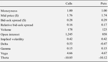
Table 1 reports average statistics for options in our final sample. The average moneyness, defined as the ratio of the strike to the underlying price when the option is 30 days to maturity,
6
for both, calls and puts, surrounds 100%, which means that our sample is constituted by highly at-the-money contracts. The average mid-price, computed as the average of the bid and ask quotes, for calls (puts) is 1.76 (1.74) and the average bid-ask spread is 0.28 (0.29). We also compute relative bid-ask spread indicator, which is the ratio of the bid-ask spread to the mid-price, in order to attenuate discrepancies among different magnitude of option prices. The average relative bid-ask spread in our sample is 0.28 and 0.29 for calls and puts, respectively. On average, each call (put) is traded 178 (123) times per day – volume – and has 1,245 (858) open contracts outstanding per day – open interest. Implied volatility, obtained by iterative induction from Cox, Ross, Rubinstein (1979) binomial tree model, is, on average, 0.42 for both, call and put contracts. On greeks, calls’ (puts’) average delta is 0.53 (-0.47), average gamma is 0.15 (0.15), average vega is 4.66 (4.67) and, finally, average theta is -10.85 and (-10.12).
Table 1: Options summary statistics
Table 1 reports average moneyness, mid-price, bid-ask and relative bid-ask spreads, volume, open interest, and Greeks, namely delta, gamma, vega and theta, in our final sample. All the measures are computed or extracted on the day the options are one month to maturity. Moneyness is defined as the ratio of the strike price to the price of the underlying security; mid-price is the average of the bid and ask quotes, bid-ask spread is the difference between the ask and bid quotes; relative bid-ask spread is the ratio of bid-ask spread to the mid-price; volume and open interest are, respectively, the traded volume and the number of contracts open; implied volatility and the greeks are obtained through Cox, Ross, Rubinstein (1979) binomial tree model. The final sample is comprised of 123,684 monthly put-call pairs for 5,116 unique stocks.
Figure 1 describes the behavior over time of options’ features for calls and puts in our final sample, namely moneyness, open interest, implied volatility, and relative bid-ask spread. Each month, we compute cross-sectional averages for each option characteristic on the day the option is 30 days to maturity, building a continuous time series of monthly averages.
Calls Puts
Moneyness 1.00 1.00 Mid price ($) 1.76 1.74 Bid-ask spread ($) 0.28 0.29 Relative bid-ask spread 0.16 0.17 Volume 178 123 Open interest 1,245 858 Implied volatility 0.42 0.42 Delta 0.53 -0.47 Gamma 0.15 0.15 Vega 4.66 4.67 Theta -10.85 -10.12
7
Panel A refers to options’ average moneyness – despite the fact we imposed a range of strike to spot prices between 0.975 and 1.025 as at-the-money range, the average moneyness in our sample closely surrounds 1 and no particular pattern can be observed throughout different economic cycles. Panel B refers to average open interest, the number of contracts outstanding – we want to point out two relevant patterns for open interest. First, we can observer that, on average, there is a considerably larger number of open call contracts outstanding, in comparison to open put contracts, which underlines the theory that overall investors support a more bullish view of the market1. Second, we can observe a scaling number of contracts, especially call options, from 2001 to 2008, the period comprised between the greatest depressions of the 21st century, the Dot-Com Bubble and the Subprime Mortgage Crisis. Panel C depicts average implied volatility distribution. It is noticeable that the largest spikes in implied volatility are nearly parallel to periods of large stock markets decline – the two largest peaks surround the Dot-Com Bubble (1995-2001), at first, and the Subprime Mortgage Crisis (2007-2010), at second. We can also observe smaller implied volatility increases in 2011 and 2016, when the stock markets dropped due to, respectively, concerns with US economic growth slowdown and the respective credit rating downgrade2 by Standard and Poor’s from AAA to AA+, and a combination of political and financial uncertainty in 2015-2016 period, namely, Chinese GDP growth slowdown, Greek debt default, the end of quantitative easing in the United States, and, finally, Brexit referendum. These patterns go in line, for instance, with findings of Goyal and Saretto (2009), who report that “investors overact to current events, increasing (decreasing)
their estimate of future volatility after large negative (positive) stock returns.” Barberis and
Huang (2001) also use their behavioral model, based on loss aversion concept3, to show that a stock’s poor performance leads investors to become more sensitive to future losses and, hence, to increase riskiness, i.e., volatility expectations for that stock. And, finally, Panel D shows the average relative bid-ask spread, which reveal an increasing pattern, ranging from 0.1 in 2001 to almost 0.4 in 2017.
Figure 1: Options characteristics through time
Figure 1 portrays the behavior of calls and puts characteristics through the sample period, January 1996 to December 2017. Panel A refers to options average moneyness, defined as the ratio between the strike price and the price of the underlying. Panel B refers to average open interest, the number of contracts opened. Panel C depicts average implied volatility distribution, interpolated from Cox, Ross, Rubinstein (1979) binomial tree model. Panel
1 By buying call options, investors are betting on rising market prices – bullish view; while, by buying put options, investors are betting on falling market prices – bearish view.
2 This event is known in investing community as Black Monday, which precisely happened on August 8th, 2011. 3 Namely that investors are more sensitive to losses than to gains.
8
D features the average relative bid-ask spread, computed as the ratio of the bid-ask spread to the mid-price. All the averages are cross-sectional, computed across all the stocks in each month. All the statistics are calculated on the day the option contracts are one month to maturity.
3. VRP-based investment strategies with options
3.1. Historical volatility and implied volatility measuresOur goal is to build investment strategies with options based on the Variance Risk Premium (VRP), which we will further define as the difference between the historical volatility of the underlying stocks’ returns and the implied volatility from the option markets. We compute the two volatility measures, the historical volatility (HV) and the implied volatility (IV), each month and for each stock. Both indicators are computed on the day the option contracts have 30 days to maturity, which is also the day of the portfolio formation.
We compute HV as an annualized4 standard deviation of stocks’ daily realized returns over the previous 252 trading days. We have previously ensured that every stock in our sample has, at least, 253 consecutive returns observations for this purpose. IV is computed as a simple
4 By multiplying the daily statistic by the square root of 252.
Panel A: Average Moneyness Panel B: Average Open Interest
9
average of the implied volatilities from the call and the put options on the same underlying security, which were previously selected through the aforementioned criteria.
It is relevant to disclose that some drawbacks could be pointed out to our approaches of computing the variance risk premium and, in particular, its components – the historical and implied volatilities. In fact, volatility estimation topic is one of the most widely discussed and debatable among the Financial academic community.
For instance, Bollerslev, Gibson and Zhou (2011) argue that the use of Black and Scholes option implied volatilities and realized volatilities from daily returns lead to biased volatility risk premium estimates. They propose a different method to estimate a stochastic measure of volatility risk premium, which they also refer as investor’s risk aversion index. They utilize a “model-free” estimation approach for both, historical and implied volatilities measures –
“Model-free historical volatilities are computed by summing squared returns from high-frequency data over short time intervals during the trading day. […] Model-free implied volatilities are computed from option prices without the use of any particular option-pricing model.” They report that these methods increase the volatility estimation accuracy and are much
simpler to implement. They also extend their analysis to include time-variation in the volatility risk premium estimation, explained by economic state variables. In other related research, Bollerslev, Tauchen and Zhou (2009) report that VRP estimated through this approach is also useful to predictor future stock market returns – “The magnitude of the predictability is
particularly strong at the intermediate quarterly return horizon, where it dominates that afforded by other popular predictor variables, such as the P/E ratio, the default spread, and the consumption–wealth ratio.”
In turn, Carr and Wu (2009) resort to variance swap concept and market prices of options to quantify the variance risk premium. Particularly, they study the behavior of VRP for five stock indexes and 35 individual stocks. A variance swap is an “over-the-counter contract that
pays the difference between the standard realized variance estimate and a fixed variance swap rate.” Since a swap does not have a cost at initiation of the contract, the variance swap rate can
be interpreted as a risk-neutral estimate of the future volatility. Given this understanding, they define the variance risk premium as the difference between the ex post realized volatility and a synthetic variance swap rate, build from a linear combination of option prices.
Following on the approach followed in our analysis, undertook by Goyal and Saretto (2009), Table 2 presents summary statistics on HV and IV in our sample, as well as on the
10
monthly changes in the two volatilities measures. We firstly compute time-series statistics, namely, the mean, standard deviation, minimum, maximum, skewness and kurtosis, of the four measures, and then report the cross-sectional averages of these statistics, which can be interpreted as the average characteristics of an average stock.
Table 2: HV and IV summary statistics
Table 2 describes the summary statistics on HV and IV in our sample, as well as on the monthly changes in these two volatility measures. We firstly compute time-series statistics, namely, the mean, standard deviation, minimum, maximum, skewness and kurtosis, of the four measures, and then report the cross-sectional averages of these statistics. For each month and each stock, HV is the annualized standard deviation of stocks’ daily realized returns over the previous 252 trading days, and IV is a simple average of the implied volatilities from the call and the put options on the same security and on the same day, previously selected as described in Section 2.1.
HV and IV are very similar to each other, with both mean values of about 46.7%, and median values only differing by 0.001 percentage points. This fact is, however, inconsistent with the existing literature that reports that the implied volatility exceeds, on average, the historical volatility, suggesting negative volatility risk premiums [Jackwerth and Rubinstein (1996) and Bakshi and Kapadia (2003)]. Similar to findings of Goyal and Saretto (2009), implied volatility is more volatile, with a standard deviation of 14.1%, against 13% for historical volatility, as well as more positively skewed and with a higher probability of extreme values than HV. Also, and again, in accordance to the referred research, the monthly changes in both volatility measures are almost null, although changes in implied volatility are more substantial. The largest spike in implied volatility in our sample is for Vanda Pharmaceuticals Inc. (Nasdaq: VNDA), a biopharmaceutical company, which went from trading at an ATM IV of 74% to 276%, and declined c.40% in share price, from September to October 2013. This period surrounded company’s third quarter earnings release, which goes in line with Dubinsky and Johannes (2005), who report that Implied Volatility for individual stocks increases on earnings announcements.
Mean Median Std. Dev Min Max Skewness Kurtosis
HV 0.467 0.444 0.130 0.327 0.722 0.696 3.795
IV 0.467 0.443 0.141 0.309 0.786 0.920 4.765
Δ HV 0.000 0.000 0.026 -0.037 0.039 0.128 6.134
11
3.2. Portfolio formation
Each month, we divide the underlying stocks in equal-weighted decile portfolios on the basis of the volatility risk premium. We compute this measure for each stock on the day the option contracts are 30 days to maturity, and we assign securities to decile portfolios on the same day – portfolio formation date. The lowest decile (1) is composed by stocks with the highest negative difference between the two volatilities metrics, while the highest decile (10) is composed by stocks with highest positive difference. Each month we have on average 535 stocks assigned across the decile portfolios, with the lowest number of stocks per month being 262 and the highest 895. We do not verify particular industry over-concertation in any of the decile portfolios, measured through SIC codes relative presence in each portfolio. However, we can distinguish SIC codes 67 – Holding and Other Investment Offices, 73 – Business Services, and 28 – Chemicals and Allied Products, that are, respectively, the first, second and third largest presence throughout the ten portfolios. They together account, on average, for c.25% of securities across the decile portfolios, and increase their relative frequency in the extreme portfolios, namely 30.5% in portfolio 1 and 28.2% in portfolio 10. This means that securities in these industries have more extreme mismatches in investors’ expectations about future returns volatilities.
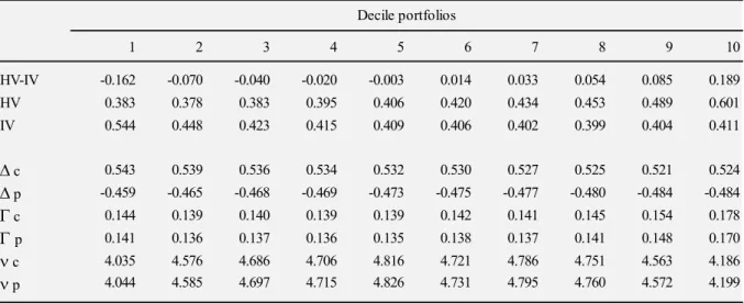
Table 3 describes summary statistics across the decile portfolios, namely the average HV, average IV, average difference between HV and IV, as well as the average values for greeks across the ten portfolios. Each month and inside each portfolio, we firstly compute the cross-sectional averages for each of the referred statistics, building a continuous time-series of portfolio statistics, and then report the time-series averages.
We find that HV and IV move in opposite directions as one proceeds from decile 1 to decile 10. The average historical volatility is 38.3% in decile 1 and steadily increases through higher deciles, up to reach 60.1% in decile 10. In turn, average implied volatility is 54.4% in decile 1 and decreases up to 41.1% in portfolio 10. As such, the average difference between the historical and the implied volatilities increases from negative 16.2% in portfolio 1 to 18.9% in portfolio 10. We find that this regularity can be related to the underlying stocks’ returns in the month prior to the portfolio formation. In Figure 2, we can observe that stocks in decile 1 have, on average, negative returns, while stocks in decile 10 have, on average, positive returns in the month prior to portfolio formation. This goes in line with the findings of Goyal and Saretto (2009), who associate this pattern to investors’ overreaction to short-term events – they suggest that investors “increase (decrease) their estimate of future volatility after negative (positive)
12
stock returns.” They actually take a step further and explore the forecasting power of implied
volatility measure in terms of predicting future volatility of returns. They report a negative forecasting error, measured as the difference between the actual observed value and the estimate, for decile 1, and a positive forecasting error for decile 10. Once again, this is justified by investors’ overreaction to positive (negative) news by underestimating (overestimating) future volatility of stock returns. Our analysis is, in fact, strongly motivated by these overreactions, which are on the basis of the further reported abnormal returns.
Concluding the analysis of Table 3, the values for options’ greeks do not present much variability across the deciles. Average delta for calls surrounds 0.53, while average delta for puts is close to -0.47. Average gamma and vega for both, calls and puts, are, respectively, 0.14 and 4.59.
Table 3: Decile portfolios formation date summary statistics
Each month, stocks were split in equal-weighted decile portfolios on the basis of the volatility risk premium (VRP), defined as the difference in HV and IV. Table 3 describes summary statistics across the decile portfolios, namely the average HV, average IV, average difference between HV and IV, as well as the average values for greeks across the ten portfolios. We firstly compute cross-sectional averages of these statistics, for each month and inside each portfolio, building a continuous time-series of portfolio statistics, and then report time-series averages of the same statistics.
Figure 2: Stocks returns in the month previous to portfolio formation
Figure 2 maps the time-series of returns of the underlying stocks in decile portfolios 1 and 10, in the month prior to their inclusion in the respective portfolio. For each decile and each month in our sample, we compute cross-sectional averages of stock returns, building a continuous time-series of underlying stock returns. Figure 2 then presents this time-series.
1 2 3 4 5 6 7 8 9 10 HV-IV -0.162 -0.070 -0.040 -0.020 -0.003 0.014 0.033 0.054 0.085 0.189 HV 0.383 0.378 0.383 0.395 0.406 0.420 0.434 0.453 0.489 0.601 IV 0.544 0.448 0.423 0.415 0.409 0.406 0.402 0.399 0.404 0.411 D c 0.543 0.539 0.536 0.534 0.532 0.530 0.527 0.525 0.521 0.524 D p -0.459 -0.465 -0.468 -0.469 -0.473 -0.475 -0.477 -0.480 -0.484 -0.484 G c 0.144 0.139 0.140 0.139 0.139 0.142 0.141 0.145 0.154 0.178 G p 0.141 0.136 0.137 0.136 0.135 0.138 0.137 0.141 0.148 0.170 n c 4.035 4.576 4.686 4.706 4.816 4.721 4.786 4.751 4.563 4.186 n p 4.044 4.585 4.697 4.715 4.826 4.731 4.795 4.760 4.572 4.199 Decile portfolios
13
Figure 3: HV-IV spread through time
Figure 3 shows the behavior of the spread between the historical and implied volatilities through time, for each decile portfolio. The portfolios were built as in Table 3. Each month and inside each portfolio, we compute cross-sectional averages of HV-IV spread, building a continuous time-series for this statistic.
Figure 3 depicts the behavior of the spread between the historical and the implied volatilities for each decile portfolio through time. We can observe that the average spread ranges around 0.2 percentage points around zero, for periods excluding large stock market declines, and significantly increases in those periods. At the time of the Dot-Com Bubble, for example, the spread almost doubles, going from near -0.4, for decile 1, to close to 0.4, for decile 10. It goes beyond |0.5| mark during the Subprime Mortgage Crisis.
-.4 -.2 0 .2 .4 .6 1996 1998 2000 2002 2004 2006 2008 2010 2012 2014 2016 2018
Panel A: Stock Returns in Decile 1
-.2 0 .2 .4 .6 1996 1998 2000 2002 2004 2006 2008 2010 2012 2014 2016 2018
14
3.3. VRP-based investment strategies with options
We build three types of options strategies based on the volatility risk premium: (1) straddles portfolios; (2) Delta-Hedged Calls portfolios; and (3) Delta-Hedged Puts portfolios. These strategies allow us to limit the directional exposure risk5 and to take advantage of the volatility mispricing. The straddles portfolios are built by combining one long call and one long put, with the same underlying security, the same strike price and the same maturity date. The Delta-Hedged Calls portfolios are built by going long on a call option and going short on delta shares of the underlying security. And, finally, the delta-hedged put portfolios result from buying a put option and buying delta shares of the underlying security. As before mentioned, the deltas were previously extracted from the OptionMetrics Ivy DB.
4. VRP-based investment strategies returns and controls for risk
4.1. Portfolios’ returns measuresThe portfolio returns are computed on option contracts maturity, 30 days after the portfolio formation, with the assumptions that all the option contracts are settled in cash. Most of the contracts, c. 80%, mature on the third Saturday of the maturity month. Being Saturday a no-trading day, there is no quote for the underlying stock price on that day. In these cases, we overcome this problem by considering, for portfolios’ returns calculation purposes, the quoted
5 Risk that arises from the exposure to the underlying asset’s price movements
15
prices from the last Friday before the expiration Saturday. Technically, this is not wrong, since in-the-money options would automatically be exercised at the Friday’s 4 p.m. closing price, although would only be settled by midday of the following Saturday. For each stock, in each month, the return (𝒓𝒊𝑻) is computed through the following formula:
𝒓𝒊𝑻= 𝑷𝒊𝑻 𝑷𝒊𝒕 − 𝟏
Where (𝑷𝒊𝒕) is the initial price of the strategy on the portfolio formation day (t) – 30 days
before the maturity, and (𝑷𝒊𝑻) is the strategy’s price/payoff on option contracts’ maturity date (T). Although our sample is composed by American style options, we ignore the possibility of
early exercise for simplicity. By holding the option until maturity, we can claim to be conservative in our analyses, since we are not taking advantage of the early exercise opportunity, which could be advantageous for the investor.
For Straddles portfolios: the initial price (𝑷𝒊𝒕) is the sum of the call and the put prices, which, in turn, are computed as the average price between the respective ask and bid quotes; the price at maturity (𝑷𝒊𝑻) is the payoff from exercising the option that expires in-the-money. As such, the payoff at maturity depends on the underlying price on the date – we use the underlying’s closing price for returns calculation purposes – and the options’ strike price.
For Delta-Hedged Calls portfolios6: the initial price (𝑷
𝒊𝒕) is the average of the bid and ask quotes of the call option less the proceeds received from short-selling delta shares of the underlying security; the price at maturity (𝑷𝒊𝑻) is the payoff from exercising the call option, if
this expires in-the-money, less the costs incurred to cover the short position, by buying delta shares of the underlying security. To compute the proceeds from short-selling, the payoff from option exercise, and the costs to cover the short position, we value the underlying stocks at its closing quote on the respective day. Moreover, we consider delta to hold constant throughout the holding period.
After computing the returns with the aforementioned approaches for individual securities and the respective strategies, we calculate cross-sectional, equal-weighted averages of those returns, for each decile portfolio and each month. In this way, we build a continuous time-series
6 A similar approach is followed for calculations of delta-hedged puts returns, with the following exceptions: (1) The initial price is the sum of the option cost and the cost incurred to buy delta shares of the underlying
stock.
(2) The price at maturity is the payoff from exercising the in-the-money put option and the proceeds received from selling the delta shares of the underlying stock.
16
of VRP based option strategies’ returns, for each decile portfolio. Table 4 reports time-series summary statistics of these returns for the ten decile portfolios, as well as for the spread portfolio (10-1), which is the zero-cost strategy portfolio – formed by taking a long position in securities that belong to portfolio 10 and short selling the securities from portfolio 1. We report the standard summary statistic: mean, standard deviation, minimum, and maximum, as well as two measures of risk-return trade-off: Sharpe Ratio (SR) and Certainty Equivalent (CE). All the reported statistics should be interpreted in monthly terms.
We want to point out that Sharpe Ratio, although being a standard statistic of risk-return trade-off, has been reported by several authors as not the best measures to evaluate the performance in options involving context, mainly due to options’ returns “extreme statistical
nature generated by nonlinear nature of payoffs” [Broadie et. al (2009)]. In particular,
Ingersoll, Spiegel, Goetzmann, and Welch (2007) analyze how different performance measures can be gamed by their direct beneficiaries, with a special attention for the Sharpe Ratio. They also develop and present a manipulation-proof measure, and apply their findings in the specific context of hedge funds, where derivatives use is particularly popular.
The main problem associated to the Sharpe Ratio remains the fact that it only considers the first two moments of the returns’ distribution, the mean and the standard deviation, which is particularly ill suited to characterize options returns. We find Certainty Equivalent as a better method to assess the risk-return characteristics, since it considers all the moments of the returns’ distribution.
CE was computed through the below stated formula, using a power utility function with constant relative risk-aversion parameter (, following Brand (1999).
𝑪𝑬 = [(𝟏 − 𝜸)𝑼̅]
𝟏
(𝟏−𝜸)− 𝟏
Where 𝑼̅ is the time-series average of the CRRA utility function for each month in each decile portfolio. We set the risk aversion parameter equal to 3 and to 7, relying on findings of Bliss and Panigirtzoglou (2004). The authors use the information provided by the option markets, as well as securities’ market prices to build a term structure of risk preferences. They use option prices to build probability density functions (PDF), which, by construction, are risk-neutral, that are then tested for the ability to accurately estimate density forecasts, i.e., to reflect market expectations about the underlying asset. The risk aversion coefficient is considered to be on the basis of the potential mismatch, if exists, between this risk-neutral forecast and the
17
objective forecast, derived from the realized densities. This difference is used to “infer the
degree of the risk aversion of the representative investor.” Although their studies on estimated
risk aversion coefficient are in respect to S&P500 and FTSE100 indexes, we rely in their results, in particular for the S&P500, to proceed with our research. They report an estimated risk aversion coefficient of 4 for the S&P500 index, 4 weeks investment horizon, and a power utility function. By taking a risk aversion coefficient of 3 and 7 in our own study, we are going slightly more optimistic (3) and significantly more conservative (7) in our assessment of our investors’ risk aversion.
Panel A reports the statistics for returns from the Straddles strategy. We can observe that these returns present an increasing pattern when one moves from the lower to the higher decile portfolios, with the mean return going from -8.8% for portfolio 1 to 4.7% for portfolio 10. Looking at the volatility, it ranges from 22.5% to 31.7% per month and there is no specific pattern across portfolios. The minimum monthly return is 61.3% in decile 4 and the maximum is 209.3% in decile 9. Our zero-cost strategy portfolio (10-1) earns a monthly average return of 13.5% and has an average monthly volatility of 26.7%. As such, the monthly Sharpe Ratio, computed as the ratio of average return to volatility of returns, is 0.498, which resembles to an annual SR of 1.75. The Certainty Equivalent (annualized CE) with risk aversion coefficient equal to 3 is equal to 1.8% (21.3%) while it is equal to -0.259 (-310.7%) for a risk aversion coefficient of 7. The negative Certainty Equivalent in the second case can be justified by very large drawdowns, with the maximum monthly loss being 66.6%, and a high risk aversion coefficient. It means that a averse investor would prefer to invest his wealth on the risk-free asset instead of investing in the respective strategy.
Panel B reports the statistics for returns from the Delta-Hedged Calls strategy, and Panel C reports for Delta-Hedged Puts strategy. The magnitude of returns for these two strategies is much lower compared to the Straddles return. This fact is not surprising, and ca be justified by two reasons. First, Straddles are composed by two options, which allows the strategy to take advantage from the mispricing of both options, while Delta-Hedged Calls and Delta-Hedged Puts only benefit from the mispricing of one option – a call or a put, respectively. Second, both Delta-Hedged strategies involve a position in the underlying security, for which we do not claim the existence of mispricing. Despite these facts, we can still observe an increasing pattern in average returns as one moves from the lower to the higher decile. For both Delta-Hedged strategies, decile 1 has an average negative monthly return, while decile 10 has an average positive monthly return. As following, the spread (10-1) zero-cost portfolio from the
Delta-18
Hedged Calls (Puts) strategy, yields an average monthly return of 1.3% (1.7%) and has a monthly volatility of 2.9% (2.6%). Despite low returns, Sharpe Ratios are very high for both strategies due to the low standard deviation, namely 1.5 (2.3) yearly. Finally, the Certainty Equivalent is positive for both strategies even for a more risk averse investor, mainly due to absence of extreme gains or losses – the maximum monthly gain is 15.2% (12.3%) and the maximum monthly loss is 6.4% (6.3%).
Table 4: Portfolios returns summary statistics
Table 4 describes summary statistics on returns from VRP-based investment strategies with options. Panel A reports the statistics for Straddles strategy, Panel B reports for Delta-Hedged Calls strategy, and Panel C reports for Delta-Hedged Puts strategy. The portfolios were built as described in Section 3.2. The spread portfolio (10-1) is the zero-cost strategy portfolio – formed by taking a long position in securities from portfolio 10 and short selling securities from portfolio 1. Each month we build a continuous time-series of VRP-based option strategies returns for each decile portfolio. Table 4 then reports time-series summary statistics of these returns, namely the mean, standard deviation, minimum, and maximum, as well as two measures of risk-return trade-off, the Sharpe Ratio (SR) and the Certainty Equivalent (CE). CE was computed from a utility function with constant relative risk-aversion parameter ( equal to 3 and to 7.
1 2 3 4 5 6 7 8 9 10 10-1 Mean -0.088 -0.037 -0.021 -0.017 0.001 0.000 -0.001 0.011 0.020 0.047 0.135 Std. Dev 0.225 0.261 0.253 0.264 0.317 0.294 0.293 0.318 0.301 0.314 0.267 Min -0.514 -0.583 -0.552 -0.613 -0.506 -0.547 -0.503 -0.547 -0.477 -0.447 -0.666 Max 1.071 1.383 1.420 1.502 1.767 1.818 1.938 1.967 2.093 1.776 1.509 SR -0.397 -0.150 -0.089 -0.072 -0.002 -0.006 -0.010 0.030 0.060 0.144 0.498 CE (=3) -0.155 -0.120 -0.105 -0.103 -0.097 -0.101 -0.096 -0.088 -0.076 -0.055 0.018 CE (=7) -0.226 -0.222 -0.216 -0.226 -0.183 -0.214 -0.198 -0.192 -0.168 -0.152 -0.259 Mean -0.006 -0.001 0.001 0.000 0.002 0.002 0.001 0.003 0.004 0.007 0.013 Std. Dev 0.029 0.030 0.030 0.029 0.032 0.033 0.031 0.033 0.033 0.036 0.029 Min -0.069 -0.074 -0.076 -0.072 -0.067 -0.059 -0.047 -0.067 -0.046 -0.051 -0.064 Max 0.153 0.196 0.179 0.196 0.206 0.210 0.228 0.192 0.210 0.240 0.152 SR -0.252 -0.094 -0.007 -0.055 0.007 0.006 -0.014 0.041 0.078 0.148 0.380 CE (=3) -0.007 -0.002 0.000 -0.001 0.001 0.000 0.000 0.002 0.003 0.005 0.012 CE (=7) -0.008 -0.004 -0.001 -0.002 -0.001 -0.001 -0.002 0.000 0.001 0.003 0.010 Mean -0.014 -0.006 -0.003 -0.003 -0.001 -0.002 -0.002 -0.001 0.000 0.003 0.017 Std. Dev 0.026 0.028 0.026 0.027 0.032 0.029 0.028 0.028 0.028 0.031 0.026 Min -0.086 -0.091 -0.096 -0.086 -0.085 -0.072 -0.065 -0.081 -0.061 -0.070 -0.063 Max 0.107 0.150 0.138 0.153 0.182 0.156 0.163 0.146 0.156 0.174 0.123 SR -0.590 -0.277 -0.178 -0.186 -0.083 -0.125 -0.128 -0.087 -0.052 0.041 0.579 CE (=3) -0.015 -0.007 -0.004 -0.004 -0.002 -0.003 -0.003 -0.002 -0.001 0.002 0.016 CE (=7) -0.016 -0.008 -0.005 -0.006 -0.004 -0.004 -0.004 -0.003 -0.002 0.000 0.015
Panel C: Delta-hedged put returns Portfolios
Panel A: Straddles returns
19
We also show a time-series of average returns from the zero-cost portfolios of the three strategies in Figure 4. We can observe that all the strategies follow a similar pattern throughout time, although Straddles strategy returns are much more substantial in magnitude. Overall, the returns seem to follow almost in parallel the global equity market performance, with increasing periods prior to the major, aforementioned, crashes and major declines during those. As already mentioned, the increasing (decreasing) returns also coincide with periods of high (low) volatility. The major spikes in returns were observed between 1998 and 2002, also the period of the most significant declines for our strategies. It is worthwhile to mention that Delta-Hedged Calls strategy seems to be less impacted than the other two during the periods of the stock market’s decline, since investor’s position is hedged by a short position on the underlying. The worst performance for Straddles and Delta-Hedged Calls strategies comes around 2004, a period of relatively low volatility. For Delta-Hedged Puts strategy, the worst period is during the Subprime Mortgage Crisis, which is justifiable by the strategy’s exposure to a long position in the underlying.
Figure 4: Spread portfolio (10-1) returns over time
Figure 4 maps the time-series of average returns from the zero-cost portfolios of the three strategies. For each month, we compute the cross-sectional average of returns, building a continuous time-series of average monthly returns for strategy’s zero-cost portfolio. Panel A presents the time-series of returns from the Straddles strategy, Panel B reports for the Delta-Hedged Calls, and Panel C for Delta-Hedged Puts strategies.
-.5 0 .5 1 1. 5 1996 1998 2000 2002 2004 2006 2008 2010 2012 2014 2016 2018
20
4.2. Risk-adjusted returns
Our goal now is to test whether the presented returns persist above risk related factors, i.e., whether the returns driven by our strategies can be considered abnormal. Since the options in the sample are derivative instruments on individual equity securities, our intuition is that our returns depend, at least, on the same sources of risk as the returns of the equity securities. To test whether our returns can be explained by any of the industry standard risk factors, we run two regressions for each strategy. We firstly regress the returns of the spread portfolios (10-1) on the Market Risk Premium factor only, and then on Fama and French (1993) three factors, as well as Carhart (1997) momentum factor. We obtain all the data on the aforementioned risk factors form Fama and French data library. In these regressions we are not only interested in
-.0 5 0 .0 5 .1 .1 5 1996 1998 2000 2002 2004 2006 2008 2010 2012 2014 2016 2018
Panel C: Delta-Hedged Puts Spread Portfolio Returns Over Time
-.0 5 0 .0 5 .1 .1 5 1996 1998 2000 2002 2004 2006 2008 2010 2012 2014 2016 2018
21
the significance of the coefficients related to each of the factors, but also, and mainly, in the value and significance of the intercept. The intercept can be interpreted as the Jensen’s alpha (1968), namely, portfolio’s abnormal return over the theoretical expected returns, predicted by the risk-adjusted model. Table 5 reports the estimated values of the coefficients associated to each of the aforementioned factors, as well as the adjusted coefficient of determination associated to each regression. The values in parentheses represent the t-statics of each coefficient and the values with the asterisk correspond to coefficients that are statistically significant at 5% level.
Firstly, we can observe that all the strategies show significant negative loadings on the market risk premium factor, which means that, on average, an increase in MRP leads to a decrease in the returns of our strategies. Secondly, we can observer that Fama and French factors, as well as Momentum factor are statistically insignificant to explain Straddles and Delta-Hedged Calls portfolios’ returns, while Delta-Hedged Puts portfolios show a significant loading on the size factor. This last observation can be justified by the fact that a Delta-hedged put portfolio involves a long position on the underlying asset, which, as documented in the literature, has a significant loading on the SMB factor. In turn, the negative coefficient can be interpreted as a sign that our portfolios tilt on firms with larger capitalizations. Moreover, we testify that our strategies generate positive and significant alphas, which are very close to the average raw returns.
Table 5: Risk-adjusted returns
We regress the returns of the spread portfolios (10-1) from each strategy – Straddles, Delta-Hedged Calls and Delta-Hedged Puts – firstly, on the Market Risk Premium factor only [regressions (1), (3), and (5)], and then on Fama and French (1993) three factors (Mkt-Rf, SMB, HML) and Carhart (1997) momentum factor (MOM) [regressions (2), (4), and (6)]. Table 5 reports the estimated values of the coefficients associated to each of the aforementioned factors, as well as the adjusted coefficient of determination associated to each regression. The values in parentheses represent the t-statics of each coefficient and the values with the asterisk correspond to coefficients that are statistically significant at 5% level.
22
We also test the significance of our returns in regard to two measures of aggregate volatility factor, namely the Aggregate Jump and the Volatility Risk, both most recently developed in Cremers, Halling, and Weinbaum (2015).7 Authors’ main goal was to study
“Whether the aggregate jump and volatility constitute separately priced risk factors”, being
Aggregate Jump, the risk of tail (or extreme) events, such as big financial turmoil, and Aggregate Volatility, the exposure of a security to market aggregate volatility. In fact, one of their main contributions was to separate the two measures, usually interpreted as one single factor in previous studies, as in Ang, Hodrick, Xing and Zhang (2006) and Bakshi and Kapadia (2003), mainly to the empirical challenge of executing the separation. They achieve this goal by setting up “investable option trading strategies that load on one factor but are orthogonal
to the other”, namely they resort to long/short strategies involving delta neutral straddles, as
these are sensitive to volatility. To proxy Jump risk factor, they set up portfolios of market neutral, vega neutral, gamma positive straddles portfolios, while to proxy Volatility risk factor, they build market neutral, gamma neutral, vega positive straddles portfolios.
We run two regressions on each of our three strategies, combining the Jump and the Volatility factors with the simple Market Risk Premium model and the Fama and French and Carhart model. Unfortunately, we only have data for Jump and Volatility, once again, kindly provided by Mr. Cremers and Mr, Halling, up to 2012. Table 6 reports the estimated values of the coefficients associated to each of the referred factors, as well as the adjusted coefficient of determination associated to each regression. The values in parentheses represent the t-statics of
7 We want to express our gratitude to Mr. Cremers and Mr. Halling, who have kindly provided us with the necessary data on the factors.
(1) (2) (3) (4) (5) (6) Alpha 0.145* 0.145* 0.014* 0.014* 0.018* 0.018* (8.93) (8.86) (7.85) (7.83) (10.90) (10.73) Mkt-Rf -1.73* -1.494* -0.187* -0.168* -0.136* -0.101* (-4.78) (-3.80) (-4.75) (-3.92) (-3.77) (-2.58) SMB - -0.79 - -0.101 - -0.104* (-1.58) (-1.85) (-2.09) HML - -0.86 - -0.071 - -0.030 (-1.59) (-1.21) (-0.56) MOM - 0.01 - 0.023 - 0.056 (1.64) (0.64) (1.73) 0.08 0.11 0.08 0.10 0.05 0.08
23
each coefficient and the values with the asterisk correspond to coefficients that are statistically significant at 5% level. The Jump factor, although economically very significant, especially for the Straddles strategy, it is not statistically significant to explain our zero-cost strategy returns. The Aggregate Volatility factor does not look neither economically or statistically significant. However, previous studies, namely Coval and Shumway (2001) and Goyal and Saretto (2009), have documented that similar to our strategies are significantly sensitive to the volatility factor, at least.
Table 6: JUMP and VOL adjusted returns
We regress the returns of the spread portfolios (10-1) from each strategy – Straddles, Delta-Hedged Calls and Delta-Hedged Puts – firstly, on the Market Risk Premium, Jump and Aggregate Volatility factors [regressions (1), (3), and (5)], and then on Fama and French (1993) three factors (Mkt-Rf, SMB, HML), Carhart (1997) momentum factor (MOM), as well as Jump and Aggregate Volatility factors [regressions (2), (4), and (6)]. Table 6 reports the estimated values of the coefficients associated to each of the aforementioned factors, as well as the adjusted coefficient of determination associated to each regression. The values in parentheses represent the t-statics of each coefficient and the values with the asterisk correspond to coefficients that are statistically significant at 5% level.
We just showed that our options strategies returns are not directly related to any of the industry standard sources of risk. As previously mentioned, options’ non-linear payoffs make it difficult for linear factor models to describe option returns. Several authors have been providing different alternatives methods to compare statistical significance of returns generated by options strategies. In particular, Broadie et. al (2009) perform a study on Index options returns and propose to evaluate significance of options returns by comparing “observed
(historical) option returns to those generated by commonly used option pricing models.”
(1) (2) (3) (4) (5) (6) Alpha 0.148* 0.150* 0.013* 0.014* 0.018* 0.018* (7.72) (7.46) (5.78) (5.88) (8.78) (8.84) Mkt-Rf -1.562* -1.245* -0.200* -0.174* -0.130* -0.086 (-3.62) (-2.72) (-4.07) (-3.33) (-2.99) (-1.86) SMB - -1.274 - -0.135 - -0.144* (-1.74) (-1.28) (-2.41) HML - -1.356 - -0.095 - -0.055 (-1.61) (-1.37) (-0.89) MOM - 0.736 - 0.039 - 0.079 (1.59) (0.95) (1.86) JUMP 16.939 14.012 -0.168 -0.757 1.032 0.492 (1.04) (0.86) (-0.09) (-0.40) (0.63) (0.30) VOL 0.442 0.526 0.046 0.054 0.061 0.070 (1.11) (1.35) (1.02) (1.21) (1.52) (1.79) 0.10 0.16 0.10 0.13 0.08 0.13 Delta-hedged puts
24
Specifically, they use as benchmarks Black-Scholes, Merton, and Heston models without priced jump risk or stochastic volatility risk. Their intuition relays on the fact that option pricing models take into consideration non-linear options’ payoffs and should, as such, provide better explanation of returns than that provided by standards liner empirical asset pricing models. Another particularly interesting study was performed by Leland (1999), who proposes a modification, based on the Rubinstein (1976) equilibrium model, to the linear factors models that result in the “correct risk measurement for portfolios with arbitrary return distributions” and eliminate abnormal returns for all fairly priced option contracts.
4.3 Risk measures for Straddles portfolios
Figure 5 presents the time-series of average options’ risk measures for Straddles strategy, in portfolios 1 and 10. For each decile and each month in our sample, we firstly compute the average between the call and the put value of each risk measure, namely, delta, gamma, and
vega, and, then, compute the cross-sectional averages of these averages. From Panel A, we can
observe that delta, which measures the sensitivity of the options’ value to price changes of the underlying security, is very close to zero for both portfolios. This means, that our Straddles strategy is almost delta-neutral, with very low risk exposure to appreciation or depreciation in the underlying. Panel B depicts the time-series for average gamma, the second derivative of the option value in respect to the underlying price and a measure of options’ value sensitivity to non-linear changes in the price of the underlying. Gamma ranges, on average, between 0.1 and 0.3 for our Straddles portfolios, with a spike around 2011. Panel C shows the evolution of the average vega through time. Vega measures the sensitivity of the options’ value, in absolute terms, to changes in volatility of the underlying security. Vega is very high for our Straddles strategies, ranging from 2 to almost 7 thought time, since Straddles are strategies that highly depend on the volatility of the underlying stocks. We can observe that vega spikes around 2001 and 2008, the already mentioned stock market crushes and periods of high market volatility.
25
Figure 5: Portfolios risk measures time-series
Figure 5 presents the time-series of average options’ risk measures, measured through option greeks, which, in turn, are calculated from the Black and Scholes model, in portfolios 1 and 10. For each decile and each month in our sample, we firstly compute the average between the call and the put value of each risk measure, and, then, compute the cross-sectional averages of these averages. Figure 5 then presents the time-series of average options greeks for deciles 1 and 10: Panel A shows average Delta, Panel B shows average Gamma, and Panel C shows average Vega. -.0 5 0 .0 5 .1 1996 1998 2000 2002 2004 2006 2008 2010 2012 2014 2016 2018 Decile 1 Decile 10
Panel A: Average Delta
0 .1 .2 .3 .4 1996 1998 2000 2002 2004 2006 2008 2010 2012 2014 2016 2018 Decile 1 Decile 10
26
4.4. Transaction costs effects on raw and risk-adjusted returns
It has been for long documented in previous studies that trading with options involves high transaction costs [Figlewski (1989), George and Longstaff (1993), Ofek, Richardson, and Whitelaw (2004), and Saretto and Santa-Clara (2009)]. As such, it is crucial for us to understand to what extent these market frictions could prevent an investor of making a profit by executing our investment strategies. We focus our analysis on transaction costs by studying the impact of the bid-ask spread on our transactions. We disregard the existence of margin requirements, which is also an important component of trading with options.
Up to now, we have been using the mid-point price to buy options and the closing price of the day to buy or sell underlying stocks. To incorporate the bid-ask spread in our investment strategies execution, we initiate long positions at the ask quotes and short positions at the bid quote. This means that we are buying at the highest price and selling at the lowest price on the market, on the specific day. We also apply a similar approach to compute the options’ payoffs on maturity date, namely, we execute the cash settlement of a call option at the bid quotes and of a put option at the ask quotes. In this way, we are considering the worst case scenario and being conservative in our analysis, by minimizing the possible options’ payoffs8. With this
8 The rationale for this statement can be better visualized by looking at the options’ payoffs formula:
(1) For a Call option, the payoff is computed as the difference between the underlying stock price on maturity day and the strike price (S-K). Since we are using bid quote, which is the lowest price on the market, for S, we are minimizing the difference S-K, hence, minimizing the payoff from the option.
(2) For a Put option, the payoff is computed as the difference between the strike price and the underlying stock price on maturity day (K-S). Since we are using ask quote, which is the highest price on the market, for S, we are minimizing the difference K-S, hence, minimizing the payoff from the option.
2 4 6 8 1996 1998 2000 2002 2004 2006 2008 2010 2012 2014 2016 2018 Decile 1 Decile 10