DIFFERENTIATED RISK MODELS IN PORTFOLIO OPTIMIZATION: A COMPARATIVE ANALYSIS OF THE DEGREE OF DIVERSIFICATION AND
PERFORMANCE IN THE S ˜AO PAULO STOCK EXCHANGE (BOVESPA)
Ivan Ricardo Gartner
Received July 8, 2010 / Accepted August 26, 2011
ABSTRACT.Faced with so many risk modeling alternatives in portfolio optimization, several questions arise regarding their legitimacy, utility and applicability. In particular, a question arises involving the adherence of the alternative models with regard to the basic presupposition of Markowitz’s classical model, with regard to the concept of diversification as a means of controlling the relationship between risk and return within a process of optimization. In this context, the aim of this article is to explore the risk-differentiated configurations that entropy can provide, from the point of view of the repercussions that these have on the degree of diversification and on portfolios performance. The reach of this objective requires that a comparative analysis is made between models that include entropy in their formulation and the classic Markowitz model. In order to contribute to this debate, this article proposes that adaptations are made to the models of relative minimum entropy and of maximum entropy, so that these can be applied to investment portfolio optimizations. The comparative analysis was based on performance indicators and on a ratio of the degree of portfolio diversification. The portfolios were formed by considering a sample of fourteen assets that compose the IBOVESPA, which were projected during the period from January 2007 to December 2009, and took into account the matrices of covariance that were formed as from January 1999. When comparing the Markowitz model with two models that were constructed to represent new risk config-urations based on entropy optimization, the present study concluded that the first model was far superior to the others. Not only did the Markowitz model present better accumulated nominal yields, it also presented a far greater predictive efficiency and better effective performance, when considering thetrade-off between risk and return. However, with regards to diversification, the Markowitz model concentrated its weights in only five of the fourteen sample assets. Contrary to these two models, the maximum entropy model showed a level of diversification that was very close to the maximum level, which would be a situation that is far more in keeping with Markowitz’s diversification precepts. However, these models showed the worst results in the comparative analysis of performance.
Keywords: diversification of investments, portfolio optimization models, entropy optimization models.
1 INTRODUCTION
The model of portfolio selection proposed by Markowitz (1952) led to the Modern Portfolio Theory (MPT) and became a watershed in the area of finance. Before Markowitz’s proposal, the predominating models were based on the idea of the existence of an optimal portfolio ob-tained through the maximization of portfolio returns, more often composed of only a single asset. Markowitz argued that this idea was mistaken, since one single asset involved a high level of exposure to variability and he proved mathematically that investors should diversify their port-folios so as to reduce their risks, since a set of portport-folios existed that combined higher gains with particular levels of risk, forming an efficient frontier.
Attaining such an efficient frontier is possible because of the multiple combinations of assets, which can be obtained through mathematical programming models, the only inputs involved being the level of return and the proposed portfolios risks, which are collected based on a series of returns on the assets analyzed. This means that such an approach is characterized as a mean-variance analysis (MVA), since the average refers to the assets returns and the mean-variance is the way of measuring the risks involved.
A few years after putting forward his proposal, Markowitz (1959) himself recognized the limita-tions of considering variance as a means of measuring risk, since a symmetric measure suggests the same penalties for above and below the average deviations. The harshest criticisms leveled against this deficiency came from Sharpe (1963, 1964), which led to hisCapital Asset Pricing Modelproposal.
Authors such as Bawa (1982), Ogryczak & Ruszczynski (1999) presented portfolio optimization models that take into account symmetric risk assessment, such as expected losses and semi-variance definitions. Following this same line of thought, Steinbach (2001) presented a revision
of these models and proposed downside riskmethodologies applied to situations of multiple
periods through dynamic programming models.
Faced with so many risk modeling alternatives in portfolio optimization, several questions arise regarding their legitimacy, utility and applicability. In particular, a question arises involving the adherence of the alternative models with regard to the basic presupposition of Markowitz’s clas-sical model, in relation to the concept of diversification as a means of controlling the relationship between risk and return within a process of optimization.
This question is pertinent since, according to Rubinstein (2002), the most important aspect of Markowitz’s work was to show that it is not the asset risk that is intrinsically important to the investor, but rather the contribution that the asset makes to the total variance of the portfolio, based on its covariance with all other assets therein included.
Faced with the question of the adherence of portfolio optimization models in relation to the pre-cepts of diversification, the aim of this article is to explore the risk-differentiated configurations that entropy can provide, from the point of view of the repercussions that these have on the degree of diversification and investment portfolios performance.
The reach of this objective requires that a comparative analysis is made between models that include entropy in their formulation and the classic Markowitz model. In order to contribute to this debate, this article proposes that adaptations are made to the relative minimum entropy and to the maximum entropy, so that these can be applied to investment portfolio optimizations.
The comparative analysis was based on performance indicators, such as the Sharpe ratio and the Alpha and Beta parameters, and on a ratio of the degree of the portfolio diversifications. The portfolios were formed by considering a sample of fourteen assets that compose the IBOVESPA, which were projected during the period from January 2007 to December 2009, and took into ac-count the matrices of covariances that were formed as from January 1999. This made it possible for the covariance matrices to capture the different facets of stock market behaviour, notably dur-ing the Bull market, Bear market and Flat (or declindur-ing price) phases, with their corresponddur-ing moments of rallies and cycles of consolidation and correction.
This article is divided into four sections. The first section deals with the main theme, uncertainties and objectives. The second section presents the theoretical framework of Markowitz’s classic model and the entropy-based models, as well as its adherence to the portfolio theory. The third section presents an empirical analysis related to the application of the proposed models, focusing on a comparative analysis of how the models have been adapted to the principle of diversification, as well as the repercussions in terms of the performance of portfolios. The fourth section presents the final considerations and recommendation for future studies.
2 PORTFOLIO OPTIMIZATION MODELS:
FROM MARKOWITZ TO ENTROPY OPTIMIZATION
Managing investment portfolios has come up against increasing problems, in view of the fact that financial markets have become increasingly exposed to exogenous and endogenous factors, related to unprecedented periods of instability. In this context, selecting portfolios is a decisive factor when managing investments for any class of investors, be they mutual fund organizations, investment firms, insurance companies, financial and non-financial groups, for-profit (business) and nonprofit organizations and individual investors in general.
The Mean-Variance Analysis proposed by Markowitz (1952) provides a mechanism to select asset portfolios, based on combinations of returns and risks. The basic concept of the model is to foresee decision-making in a single-period regime, in other words, from momentt0to moment
t1and is related to risky assets.
2.1 The classic Markowitz Model: a Mean-Variance Analysis (MVA)
The classic Markowitz Model (1987) requires inputs that are extracted from the market price series of the assets analyzed. Based on these price series, a calculation is made of the returns and variances as well as the covariance between assets.
The periodic random returns are calculated based on thei−th asset series which are given from ri t,i = 1, . . . ,n,t = 1, . . . ,T, obtained from the continual formulation ofri t = ln(vi t)− ln vi t−1
, wherevi t refers to the price of thei-th asset during periodt. A calculation of the average returns of thei-th share can be defined as the geometric mean of its returns:
ˉ
ri =
" T
Y
t=1
(1+ri t)
#1/T
−1 (1)
and the set of average returns of variousi assets forms the vector:
ˉ r= ˉ r1 ˉ r2 .. . ˉ rn
Markowitz stated that it was not enough only to consider the individual characteristics of the assets, since forming a portfolio should take into account ways by which assets can be moved conjointly over a period of time. The covarianceσi j is the basic measurement of conjoint vari-ability between two assetsi andj, and is calculated by:
σi j =σji =1T ∙
XT
t=1(ri t − ˉri) rj t − ˉrj
(2)
being thatσi j =σji, whilei 6= j andσii =σy, whilei = j. If the returns of assetsi and j move in the same direction, the result isσi j >0; otherwise, the result isσi j <0.
The importance of the measurement of this conjoint variability is the strength of the diversifi-cation proposed by Markowitz, where the objective is to combine assets that move in opposite directions, so that a drop in the price of a portfolio asset can be compensated by the rise in the price of another asset within the same portfolio.
In aggregated terms, the paired relationships of n assets are incorporated into the covariance matrixV:
V=
σ11 σ12 ∙ ∙ ∙ σ1n σ21 σ22 ∙ ∙ ∙ σ2n
..
. ... . .. ... σn1 σn2 ∙ ∙ ∙ σnn
(3)
short-selling is not considered, and can be negative in the opposite case. The set of participations of assetsi in the portfoliopcompound the vector:
w= w1 w2 .. . wn
The portfolio return for thenassets can be expressed thus:
ˉ
rp= n
X
i=1 ˉ
riwi (4)
which assumes a matrix form:
ˉ
rp=w′rˉ (4′)
whererˉis the vector of the average returns of the assets analyzed.
The risk measurement of a portfolio formed byn assets is derived from the paired relationship that exists between portfolio assets, weighted by their respective weights, and can be calculated as follows:
σ2p= n
X
i=1 n
X
j=1
wiwjσi j. (5)
In terms of matrix, the covariance of a portfolio may be calculated by
σp2=w′Vw, (5′)
wherewis the weight vector,w′is the transposed weight vector andVis the previously defined covariance matrix. In order to calculate the standard deviation, all one has to do is to solve σp=
√ w′Vw.
The construction of an optimal portfolio as suggested by Markowitz can be done by means of mathematical programming models that are formed based on combinations between asset risks and returns. The basic portfolio optimization model, which uses quadratic programming, is based on minimizing portfolio risks given a certain level of portfolio return:
min w σ
2
p = w′Vw
s.t.: w′rˉ≥ ˉrpd
w′u=1
(6)
whereuis a unit vector:
ˉ
rpd is the level of the required return of a portfolio. The solution of this model for values of rˉpd in the interval betweenrˉpmin andrˉpmax results in all the portfolios being efficient. A
possible solution for the model may be found through Lagrange multipliers:
L(w, λ1, λ2)=w′Vw−λ1 w′rˉ− ˉrpd−λ2 w′u−1 (7)
Model (6) may be re-arranged so as to combine the maximum portfolio return with the same level of risk, which will result in the following nonlinear programming formulation:
max
w rˉp = w ′rˉ
s.t.: w′Vw≤σd2
w′u=1
(8)
whereσd2is the desired level of risk and a possible solution may be found through the Lagrange multipliers.
L(w, λ1, λ2)=w′ˉr−λ1
w′Vw−σd2−λ2 w′u−1 (9)
Model (8) may also be rearranged, so as to incorporate a risk aversion coefficient, which will result in the following formulation of quadratic programming:
max
w rˉp−δσ
2
p = w′rˉ−δw′Vw
s.t.: w′u=1
(10)
whereδ is a risk aversion constant and a possible solution may be found through the Lagrange multipliers:
L(w, λ1)=w′rˉ−δw′Vw−λ1 w′u−1
(11)
In all (6), (8) and (10) cases, a restriction towi ≥should be inserted for situations where short-selling is not permitted.
2.2 Extension of the Markowitz model: the sharpe model
One of the preoccupations that come after portfolio optimization is how to define the instruments that control their performance. Sharpe (1966) identified the lack of specific methodologies to measure portfolio performances, especially when dealing with mutual funds. Sharpe’s proposal was to create an index that reflected the excess return on market portfolios per unit of risk(θg = E(rp)−rf/σ ). Since the excess return is on a risk-free asset(rf), this index falls back on the point where the Capital Allocation Line (CAL) tangencies the efficiency frontier of portfolio. Thus, this index may also be used to optimize portfolios in the following way:
max
w θ= ˉrp−rf
σp = w′ˉr−rf √
w′Vw
s.t.: w′u=1
The solution to this problem results from a portfolio with a maximum Sharpe index, which is the one with the highest relation of risk and return within the assets, known as an optimal risk portfolio. This problem can be solved using the following Lagrange formulation:
L(w, λ1)=
h
w′rˉ−rf √
w′Vwi−λ1 w′u−1
(13)
The portfolio return for this optimal portfolio may be used to define the desired portfolio return (rpd), which is a constraint for the optimal portfolio reaches a given level of performance.
2.3 Entropy modeling as a risk measurement in portfolio selection
Entropy is a concept originally discussed by Ludwig Boltzmann, and upon which the Second Law of Thermodynamic is based and associated with the degree of disorder that exists in the thermodynamic systems. Shannon (1948) widened this concept to include the theory of infor-mation, when he began to use entropy to describe the quantity of information that existed on the state of a determined system or event.
The study carried out by Philippatos & Wilson (1972) was a pioneering study to try to associate Shannon’s Entropy with a measure of risk in portfolio optimization. In their proposal, the model of entropic optimization takes into account a combination of conjoint probabilities and condi-tions of asset returns, as a means of obtaining the weights system for a portfolio, the validity of which was confirmed in an empirical analysis that included a sampling of 50 randomly se-lected NYSE and Dow Jones Industrial index assets, during the period between January 1957 and December 1970. This form of entropy-based portfolio optimization was severely criticized by White (1974), whose main point of contestation related to the fact that the portfolio entropy would be independent of weights, which did not justify its use. However, Philippatos & Wilson (1974) put forward comments that were technically sustainable to justify their proposal, proving in a simple manner that the entropy of a portfolio is a function of the weights attributed to its elements.
After this controversy, this line of study on applied entropy to select portfolios seems to have lost some of its force, since Philippatos & Wilson themselves (1974, page 215) state that: “. . . amongst the disadvantages of the measures of the theory of information and the theory of finance, are the following: (1) the measure of uncertainty or entropy has not been philosophi-cally integrated into the disciplines of economy, although this has been partially integrated into the theory of choice, of conflict and general behaviour, which are typically explored by social scientists . . . ”.
More recent concerns that have stimulated renewed interest in the application of entropic op-timization in portfolio selection, is related to the fact that many of the extensions of the classic Markowitz model, including Markowitz’s model itself, have not provided convergent solutions to the principle of diversification. In accordance with Hua & Xingsi (2003) and Bera & Park (2008), entropy is an alternative means to deal with a situation in which optimization based on a mean-variance analysis (MVA) is contrary to the notion of diversification, often driving portfolios to a high concentration of weights in a small number of assets.
2.4 Portfolio optimization models that include entropy
According to Shannon’s view (1948), entropy H(X)can be defined as the quantity of avail-able information about the state of a system X =(x1,x2, . . . ,xn), with a probability vector of p(x)
P(x)= p1(x1), p2(x2), . . . ,pn(xn), where pi(xi)≥ 0 andPin=1pi(xi)=1, justify its use as a measure of uncertainty. This means that an entropyH(X)of a random variableXis defined by the equation:
H(X)= − n
X
i=1
pi(xi)lnpi(xi) (14)
Since H(X)supplies a measure of disorder in a system, or in an expected value and in a proba-bility distribution, the entropy can be used to measure a portfolio’s degree of diversification. In order to do so, considering that pi(xi)can be replaced by weightwi, the value ofH(X)is zero if the portfolio consists of only one asset and if the portfolio has a maximum value and is uniformly distributed(pi(xi)=wi =1/n).
This interpretation is based on attribute 2 of part 6 (Choice, Uncertainty and Entropy) of the study presented by Shannon (1948, page 388), which states that: “. . . if all the pi(xi)are equal (pi(xi)=1/n), thenH(X)must be a growing monotonic function ofn. With equally probably events, there is more choice, or uncertainty, if more possible events exist. . . ”. These concepts are coherent with the precepts of diversification proposed by Markowitz, which justifies studies on the use of entropy in portfolio optimization.
Although the study made by Philippatos & Wilson (1972) presented a form of calculating the conjoint entropy of assets returns, this formulation was shown to be entirely independent of the classic Markowitz model. Thus, Hua & Xingsi (2003) presented a formulation proposal in which entropy represents one shrinkage factor of weigths in the objective-function, in the following way:
min w σ
2 p−ψ
n
P
i
wilnwi = w′Vw−ψw′lnw
s.t.: w′rˉ≥ ˉrpd
w′u=1
(15)
objective-functions values; ifψ =0, one only has the optimization according to Markowitz’s original model.
The inclusion ofψ is based on the proposal put forward by Shannon (1948, page 389), which
presents an alternative way to calculate anHentropy, by using
H(X)= −K
n
X
i=1
pi(xi)lnpi(xi),
whereK is a constant positive to adjust the measure. A solution of (15) by Lagrange acquires a format:
L(w, λ1, λ2)=w′Vw−ψw′lnw−λ1 w′rˉ− ˉrpd−λ2 w′u−1 (16)
Following this same logic, entropy may be incorporated into the models presented by the equa-tions (8) and (10), in accordance with the focus analysis. Another important question related to the incorporation of entropy in objective-functions, is related to the fact that the model does not permit short-selling by obvious mathematical limitations, it being necessary to include restriction wi ≥0.
2.5 Entropy optimization models applied to portfolio selections: a contribution
The model shown in (15) presents entropy inclusion as an objective-function of Markowitz’s classic model, the entropic calculation of which refers only to the weight vectorw. The greatest problem associated with this type of formulation is its sensitivity to the magnitude of valueψ,
since the more this parameter moves away from zero (remembering thatψ ≥ 0), the greater
the impact of the entropy on the objective-function. Since the definition of this parameter is subjective, its legitimacy may be questioned, since the distribution of portfolio weights will be directly affected by the decision makers’ preferences and values.
Since revised literature on the subject still presents lacunae in the way that entropy can be in-corporated into portfolio optimization problems, this article seeks to make its contribution by presenting two alternative methodological proposals for inclusion the entropy in the portfolio op-timization. The first presents an entropic optimization model focused on weights vector, which is conditioned by a desired level of return, using the principle of the minimum relative entropy. The second deals with an entropic optimization model that conjugates the weights vector with the return vector for every asset analyzed, taking into account the maximum entropy principle.
2.5.1 Model of the minimal relative entropy applied to portfolio optimization
The relative entropyR(Q,P0), or the Kullback-Leibler divergence between twoP0andQ
dis-tributions, is defined by the relationship
RQ,P0=
n
X
i=1
and measures the inefficiency of assuming that one random variable has a P0distribution, when its true distribution is Q, and that P0 is ana prioridistribution, for which the probability
dis-tribution is uniform. Thus, P0 has maximum entropy, and Q is an a posteriori distribution.
According to R¨odder (2000), this Qdistribution is obtained based on the addition of informa-tion in the system being analyzed, since Q is a distribution that is subject to Q| = R, in that Ris the set of probabilistic restrictions, which differentiate the P0andQdistributions, orR = {Bi|Ai[xi],i =1, . . . ,I}. Thus, the conditional distribution Q{Q(Bi|Ai)=xi,i =1, . . . ,I}, may be calculated fromP0andR, by means of the following optimization problem:
Min x R
Q,P0= n
X
i=1
Q(xi)lnQ(xi)P0(xi) (18)
This formulation characterizes the principle of minimal relative entropy, which can be adapted for portfolio optimization problems. In this adaptation, an uniform distribution of the weights vectorw0(P0(wi0))is first made and a model is formulated with the objective of minimizing the relative entropy between this weights vectorw0and the new weights vectorw∗(Q(wi)), which will result from the addition of restrictions to the problem, in the following way:
min w
n
P
i=1
Q(wi)lnQ(wi)P0 w0i
s.t.: w′rˉ≥ ˉrpd
w′u=1
(19)
that can be solved by Langrange with:
L(w, λ1, λ2)=
" n
X
i=1
Q(wi)lnQ(wi)
P0w0i
#
−λ1 w′rˉ− ˉrpd
−λ2 w′u−1
(20)
Since this formulation does not operate with Neperian (Natural) logarithms, this type of problem does not accommodate short selling, making it necessary to include restrictionwi ≥0.
2.5.2 Model of the maximum entropy applied to portfolio optimization
While model (19) deals with entropy associated only with portfolio weights, it is also possible to focus on entropy especially starting from the dispersion of random returnsri t. Taking as its base the idea of the model proposed by Philippatos & Wilson (1972), but following alternative methodological procedures, it is possible to extract the vector of weightsw, based on its combi-nation with the degree of disorder of the random returnsri t.
Jessop (1999) developed an entropic optimization model to resolve this type of question, when he sought solutions to problems of a multi-attribute evaluation, taking into account the dispersion of the performance vectors of the alternatives, based on the following entropy formulation of a random vectorx:
H(X)=ln n
X
i=1
xi
!
−
" n
X
i=1
xiln(xi)
n X
i=1
xi
#
Adapting this formulation to portfolio optimization may take the following form:
max
w H(R) = ln n
P
i=1 m
P
j=1
wjaj(ri t)
!
−
(
n
P
i=1
"
m
P
j=1
wjaj(ri t)∙ln m
P
j=1
wjaj(ri t)
#
n
P
i=1 m
P
j=1
wjaj(ri t)
)
s.t.: w′u=1
(22)
whereaj(ri t) = ri t−riminrimax−rimin and refers to the normalization of random returns
ri t. This normalization is a requirement for this modeling, since the returns can assume negative values, while the entropy operations require non-negative numbers. For this reason, this model is also applied only in cases where short-selling (wj ≥ 0)is not permitted. This problem of non-linear optimization was resolved by Lagrange in the following way:
L(w, λ1, λ2) = ln n
P
i=1 m
P
j=1
wjaj(ri t)
!
−
(
n
P
i=1
"
m
P
j=1
wjaj(ri t)∙ln m
P
j=1
wjaj(ri t)
# n
P
i=1 m
P
j=1
wjaj(ri t)
)
−λ1 w′u−1
(23)
3 AN EMPIRICAL ANALYSIS
3.1 Process of sampling and selection from the period of analysis
An empirical analysis was constructed based on the returns of a sampling of assets that are negotiated on the S˜ao Paulo Stock Exchange (BOVESPA), by taking into account that the classic Markowitz model was proposed as a means to optimize only risky assets portfolios.
This sampling of assets was collected from among the IBOVESPA shares, which is the index most commonly used as a Brazilian stock market reference. On 30th March 2010, the theoretical portfolio of IBOVESPA consisted of 63 assets. It was decided to take a sampling of fourteen assets, which represented a sampling of 22.0% of the 63 assets that composed the index. In the sampling process, the shares were selected based on a uniform distribution random number generator. After the random selection of each asset, a collateral analysis procedure was carried out to check and see if the same asset had been negotiated on all of the price collection points during the period of analysis. If the asset did not meet this condition, then it was replaced by another randomly chosen asset that was likely to meet this requirement.
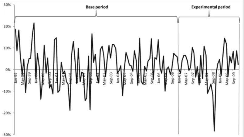
This study was carried out over the period between January 1999 and December 2009, and in-cluded a total of 132 observations for each asset. In order to ensure that this research work was operable, the research period was divided into two periods, as may be seen in Figure l.
Figure 1– Nominal Monthly Variation of the IBOVESPA during the period between January 1999 and December 2009. Source: Adapted from BMFBOVESPA (2010).
different phases, notably theBullmarket,Bearmarket andFlatmarket phases, with their corre-sponding periods ofRally, Consolidation and Correction. In order to form the monthly portfolios, the experimental period totaled a period of three years, from January 2007 to December 2009, based on the models presented in this study.
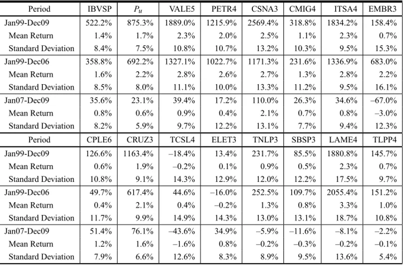
In general terms, during this whole period of ten years, there was a huge rise in the stock market nominal value of IBOVESPA listed companies, as can be seen in Table 1. The IBOVESPA (IB-VSP) reached a level of 522.2% of the nominal returns, indicating an average monthly nominal return (as per equation (1)) of 1.4%, with a standard deviation of 8.4%. Of the randomly selected sampling of fourteen bonds, there were assets that accumulated a nominal return of 2,569.42% (CSNA3), while other assets accumulated negative returns, as was the case of TCSL4 (–18.42%).
In order to identify the explicative power of the sampling, we considered a hypothetical situation whereby, on the final day of December 1998, a portfolio(Pu)was formed based on the uniform distribution of weight between the fourteen assets selected. This portfolio would have obtained a nominal accumulated return of more than 350.0%. In terms of risk, this hypothetical portfolio (Pu), would present a standard deviation (taking into account the (5) equation for the final period) almost 0.9% lower than the IBOVESPA portfolio.
Since the data in Table 1 shows a situation where a portfolio of maximumPudiversification and the IBOVESPA index present transitory relationships of risk and returns, it is understood that the empirical analysis had found an appropriate experimental base upon which to carry out a comparative analysis of the portfolio optimization models studied in this article.
Table 1– Cumulative and average returns and risk during the period between January 1999 and December 2009.
Period IBVSP Pu VALE5 PETR4 CSNA3 CMIG4 ITSA4 EMBR3
Jan99-Dec09 522.2% 875.3% 1889.0% 1215.9% 2569.4% 318.8% 1834.2% 158.4%
Mean Return 1.4% 1.7% 2.3% 2.0% 2.5% 1.1% 2.3% 0.7%
Standard Deviation 8.4% 7.5% 10.8% 10.7% 13.2% 10.3% 9.5% 15.3% Jan99-Dec06 358.8% 692.2% 1327.1% 1022.7% 1171.3% 231.6% 1336.9% 683.0%
Mean Return 1.6% 2.2% 2.8% 2.6% 2.7% 1.3% 2.8% 2.2%
Standard Deviation 8.5% 8.0% 11.1% 10.0% 13.3% 11.2% 9.5% 16.1% Jan07-Dec09 35.6% 23.1% 39.4% 17.2% 110.0% 26.3% 34.6% –67.0%
Mean Return 0.8% 0.6% 0.9% 0.4% 2.1% 0.7% 0.8% –3.0%
Standard Deviation 8.2% 5.9% 9.7% 12.2% 13.1% 7.7% 9.4% 12.3% Period CPLE6 CRUZ3 TCSL4 ELET3 TNLP3 SBSP3 LAME4 TLPP4 Jan99-Dec09 126.6% 1163.4% –18.4% 13.4% 231.7% 85.5% 1880.8% 145.7%
Mean Return 0.6% 1.9% –0.2% 0.1% 0.9% 0.5% 2.3% 0.7%
Standard Deviation 10.8% 9.1% 14.3% 12.9% 12.0% 12.2% 17.5% 9.7% Jan99-Dec06 49.7% 617.4% 44.6% –16.0% 252.5% 109.7% 2055.4% 151.2%
Mean Return 0.4% 2.1% 0.4% –0.2% 1.3% 0.8% 3.3% 1.0%
Standard Deviation 11.7% 9.9% 14.9% 14.3% 13.0% 13.1% 18.7% 10.8% Jan07-Dec09 51.4% 76.1% –43.6% 34.9% –5.9% –11.6% –8.1% –2.2%
Mean Return 1.2% 1.6% –1.6% 0.8% –0.2% –0.3% –0.2% –0.1%
Standard Deviation 7.9% 6.6% 12.6% 8.3% 8.9% 9.5% 13.6% 5.4%
Source: Adapted from the BMFBOVESPA (2010).
3.2 Analysis for Technical consideration
In order to construct an empirical analysis, four optimization models were implemented:
a) The Sharpe Model of optimization: was implemented in accordance with equation (12), so as to produce its portfolio returnrˉp, related to the level of portfolio returnrˉpdincluded in the restrictions of the other models. This procedure was adopted as a way to exogenously and objectively model the attitude of a standard-investor when faced with risk;
b) The classic Markowitz optimization model: was put into operation in accordance with equation (6), with the objective of providing a portfolio that would combine risk mini-mization that was subject to the desired performance levelrˉpd;
the difference in the levels of entropy between the distribution of uniform weight and a new distribution, in that the latter would be subject to the desired level of returnrˉpd;
d) Maximum entropy optimization model: was put into operation in accordance with equa-tion (22), with the objective of providing a weights vector that would combine the maxi-mum entropy in conjunction with the weights vectors and the random returns of the assets analyzed.
All the models were submitted to the unit restrictions of the total sum of the weights vectors and non-negativity of weights vectors, being that the latter characteristic means that short-selling is not allowed. In addition to these questions, the following should also be considered:
• All the models used operate with static programming. Although there are dynamic
pro-gramming models that can formulate projections for multiple periods, it was decided to maintain the conditions of Markowitz’s classic methodology, which means that all the portfolios were recalculated and rebalanced at the beginning of each period. The port-folios were created at the end of each month and projected for the end of the follow-ing month. For example, the initial projections for the portfolios occurred at the end of December 2006(D0)and were relative to the following month of January(D1);
• Following this system of monthly rebalancing, the covariance matrices were recalculated in each of the months of the experimental period, always using as their base the month of January 1999 and incorporating the month immediately prior to each new month projected. For example, the first portfolio projection was based on the covariance matrix calculated for the period between January 1999 and December 2006. However the second projec-tion considered the covariance matrix calculated for the period between January 1999 and January 2007. Thus, a procedure was adopted whereby the informational base of the co-variance matrices was growth over a period of time, but with a January 1999 fixed base. It was understood that this procedure made it possible for the models to incorporate more information so as to determine projections, in comparison with the situation where the size of the matrix base is constantly maintained, which occurs if the covariance base of the matrices is mobile;
• Thus, the portfolio weights were rebalanced every month based on what the models
rec-ommended, which meant that every month new information was included relating to the risk distribution involved, depending on how the covariance matrices database expanded, as mentioned previously;
• Transaction costs relating to rebalancing were not considered.
3.3 An analysis of the results of the models implemented
a) Portfolio nominal monthly return indexes (rp = P14i=1wiri t) and accumulated return indexeshr ap=Q35t=0 1+rpt
i
, formed the basis of this analysis;
b) The Sharpe Index: this was used to measure the excess return of portfolios calculated in comparison to their risk levels. This index showed their relationship to the market, when taking into account the excess return of the portfolio over the risk-free asset. This index was calculated using theθg=g(rp)−rf/σpformula, which should not be confused with the Sharpe optimization process for therˉpdcalculation (see equation (12)). As a proxy for the risk-free return raterf , the SELIC (a proxy of rate of return for Brazilian Treasury Bills) monthly rate was adopted for the date in question. The Sharpe index was used in the a priorianalysis, so as to measure the predictive efficiency of the models within the ambit of the risk and return relationship, and in thea posteriorianalysis, to measure the effective performance of the portfolios. For this second function, the formula was adapted to
θap = 1T∙ T
X
t=1
rpt −rf t
!
σ(rpt−rf t);
c) Alpha and Beta parameters: these were obtained from an analysis made of the simple linear regression between the effective portfolio returns (rpt)and the IBOVESPA returns (rmt):
rpt =α+βrmt+εt (24)
whereεt is the random error term. The purpose of an estimation of these parameters is to analyze the performance of the funds in comparison with levels of market profitability;
d) Index of the degree of portfolio diversification: this was applied based on the Goetzmann & Kumar proposal (2001):
Dt = N
X
i=1
(wi −wu)2 (25)
and was calculated for eachtperiod, wherewuwas the weight of a fully diversified market portfolio, that is to say: with a(wu =1Nu)uniform weight distribution. The lower the
Dt value, the higher the level of portfolio diversification for the period analyzed.
The optimization procedures adopted produced weights vectors for every one of the projected periods, applied in the following portfolios compositions:
p1: the portfolio composed according to the classic Markowitz Model;
p2: the portfolio constituted according to the relative minimum entropy model; and
p3: the portfolio formed according to the maximum entropy model.
The optimization procedures were implemented using the Microsoft ExcelTM SolverTM which,
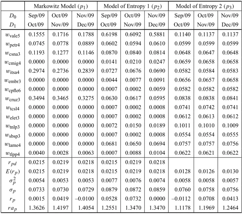
Since tabulating the results generated very extensive tables, it was decided to present a reduced graph of the results of the last quarter processed, as can be seen in Table 2. In this table, it is possible to visualize the weights calculated for the fourteen assets used in this sampling, the value of the desired return on the portfolio(rpd), that derives from the Sharpe model (12) optimization process, the return on the proposed portfolio (E(rp)), the risk value as a variance (σpy) and standard deviation(σp)of the portfolio and nominal returns obtained.
Table 2– Reduced graph of the applied optimization models.
Markowitz Model(p1) Model of Entropy 1(p2) Model of Entropy 2(p3)
D0 Sep/09 Oct/09 Nov/09 Sep/09 Oct/09 Nov/09 Sep/09 Oct/09 Nov/09
D1 Oct/09 Nov/09 Dec/09 Oct/09 Nov/09 Dec/09 Oct/09 Nov/09 Dec/09
wvale5 0.1555 0.1716 0.1788 0.6198 0.6092 0.5881 0.1140 0.1137 0.1137
wpetr4 0.0745 0.0778 0.0889 0.0602 0.0594 0.0610 0.0599 0.0599 0.0599
wcsna3 0.1193 0.1277 0.1146 0.0870 0.0840 0.0814 0.0648 0.0647 0.0648
wcmig4 0.0000 0.0000 0.0000 0.0141 0.0210 0.0247 0.0659 0.0658 0.0658
witsa4 0.2974 0.2736 0.2839 0.0727 0.0676 0.0690 0.0582 0.0584 0.0583
wembr3 0.0000 0.0000 0.0000 0.0044 0.0077 0.0091 0.0656 0.0657 0.0658
wcpfle6 0.0000 0.0000 0.0000 0.0007 0.0002 0.0059 0.0582 0.0582 0.0582
wcruz3 0.3494 0.3465 0.3275 0.0630 0.0617 0.0595 0.0838 0.0838 0.0841
wtcsl4 0.0000 0.0000 0.0000 0.0007 0.0002 0.0008 0.0741 0.0742 0.0741
welet3 0.0000 0.0000 0.0000 0.0007 0.0002 0.0008 0.0612 0.0613 0.0612
wtnlp3 0.0000 0.0000 0.0000 0.0072 0.0150 0.0189 0.1011 0.1010 0.1009
wsbsp3 0.0000 0.0000 0.0000 0.0007 0.0002 0.0008 0.0554 0.0554 0.0555
wlame4 0.0000 0.0000 0.0000 0.0681 0.0650 0.0694 0.0757 0.0757 0.0756
wtlpp4 0.0040 0.0028 0.0063 0.0007 0.0088 0.0104 0.0622 0.0621 0.0622
rpd 0.0215 0.0219 0.0218 0.0215 0.0219 0.0218
E(rp) 0.0215 0.0219 0.0218 0.0215 0.0219 0.0218 0.0128 0.0126 0.0130
σ2p 0.0054 0.0053 0.0053 0.0077 0.0076 0.0074 0.0058 0.0058 0.0057
σp 0.0733 0.0730 0.0729 0.0879 0.0872 0.0859 0.0760 0.0758 0.0756 rp 0.0015 0.0419 –0.0100 0.0528 0.0732 0.0000 –0.0112 0.0708 0.0413
r ap 1.3626 1.4197 1.4054 1.2551 1.3470 1.3470 1.1178 1.1969 1.2464
Source: Elaborated by the author.
3.3.1 An analysis of the nominal monthly and accumulated returns
The monthly nominal and accumulated returns on the portfolios proposed by models p1,p2and
p3are presented in Tables 3 and 4.
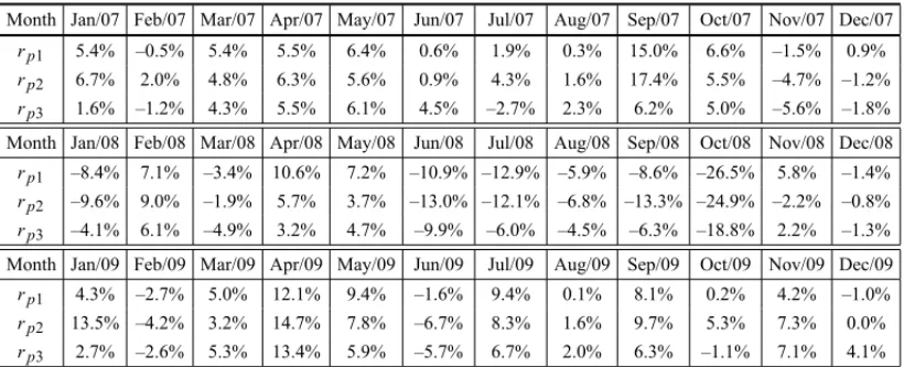
Table 3– Estimated monthly nominal returns of the portfolios.
Month Jan/07 Feb/07 Mar/07 Apr/07 May/07 Jun/07 Jul/07 Aug/07 Sep/07 Oct/07 Nov/07 Dec/07 rp1 5.4% –0.5% 5.4% 5.5% 6.4% 0.6% 1.9% 0.3% 15.0% 6.6% –1.5% 0.9% rp2 6.7% 2.0% 4.8% 6.3% 5.6% 0.9% 4.3% 1.6% 17.4% 5.5% –4.7% –1.2% rp3 1.6% –1.2% 4.3% 5.5% 6.1% 4.5% –2.7% 2.3% 6.2% 5.0% –5.6% –1.8% Month Jan/08 Feb/08 Mar/08 Apr/08 May/08 Jun/08 Jul/08 Aug/08 Sep/08 Oct/08 Nov/08 Dec/08 rp1 –8.4% 7.1% –3.4% 10.6% 7.2% –10.9% –12.9% –5.9% –8.6% –26.5% 5.8% –1.4% rp2 –9.6% 9.0% –1.9% 5.7% 3.7% –13.0% –12.1% –6.8% –13.3% –24.9% –2.2% –0.8% rp3 –4.1% 6.1% –4.9% 3.2% 4.7% –9.9% –6.0% –4.5% –6.3% –18.8% 2.2% –1.3% Month Jan/09 Feb/09 Mar/09 Apr/09 May/09 Jun/09 Jul/09 Aug/09 Sep/09 Oct/09 Nov/09 Dec/09 rp1 4.3% –2.7% 5.0% 12.1% 9.4% –1.6% 9.4% 0.1% 8.1% 0.2% 4.2% –1.0% rp2 13.5% –4.2% 3.2% 14.7% 7.8% –6.7% 8.3% 1.6% 9.7% 5.3% 7.3% 0.0% rp3 2.7% –2.6% 5.3% 13.4% 5.9% –5.7% 6.7% 2.0% 6.3% –1.1% 7.1% 4.1%
Source: Elaborated by the author.
Table 4– Nominal accumulated returns of the estimated portfolios.
Month Jan/07 Feb/07 Mar/07 Apr/07 May/07 Jun/07 Jul/07 Aug/07 Sep/07 Oct/07 Nov/07 Dec/07 r ap1 1.0544 1.0495 1.1060 1.1664 1.2406 1.2480 1.2712 1.2751 1.4664 1.5637 1.5410 1.5542 r ap2 1.0667 1.084 1.1409 1.2123 1.2804 1.2921 1.3480 1.3702 1.6084 1.6975 1.6176 1.5978 r ap3 1.0165 1.0044 1.0480 1.1053 1.1728 1.2253 1.1922 1.2200 1.2951 1.3602 1.2844 1.2607 Month Jan/08 Feb/08 Mar/08 Apr/08 May/08 Jun/08 Jul/08 Aug/08 Sep/08 Oct/08 Nov/08 Dec/08 r ap1 1.4231 1.5241 1.4728 1.6283 1.7461 1.5556 1.3553 1.2750 1.1658 0.8565 0.9066 0.8938 r ap2 1.4443 1.5750 1.5456 1.6336 1.6946 1.4747 1.2963 1.2086 1.0483 0.7876 0.7701 0.7641 r ap3 1.2093 1.2830 1.2204 1.2601 1.3199 1.1890 1.1180 1.0677 1.0006 0.8120 0.8297 0.8186 Month Jan/09 Feb/09 Mar/09 Apr/09 May/09 Jun/09 Jul/09 Aug/09 Sep/09 Oct/09 Nov/09 Dec/09 r ap1 0.9324 0.9069 0.9526 1.0683 1.1684 1.1498 1.2578 1.2586 1.3605 1.3626 1.4197 1.4054 r ap2 0.8669 0.8302 0.8570 0.9831 1.0598 0.9888 1.0704 1.0871 1.1922 1.2551 1.3470 1.3470 r ap3 0.8405 0.8190 0.8625 0.9785 1.0363 0.9771 1.0426 1.0631 1.1304 1.1178 1.1969 1.2464
Source: Elaborated by the author.
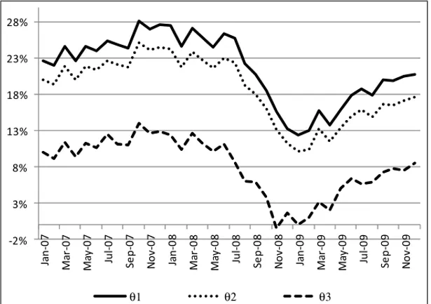
3.3.2 An analysis of the relationship between risk and return according to the Sharpe Index
The use of the Sharpe Indexa priori, as seen in Figure 2, shows that the classic Markowitz model (θ1)had the greatest predictive efficiency when compared to the minimum relative entropy(θ2)
and maximum entropy(θ3)models.
The gap between the Markowitz model and the entropy-based models were practically constant during the period analyzed, irrespective of market phases.
θ1 θ2 θ3
Figure 2– Thea priorisharpe performance indexes. Source: Elaborated by the author.
Table 5– Thea posteriorisharpe performance indexes.
p1 p2 p3
Mean(rp-rf) 0.0004 –0.0008 –0.0030
σr p-r f 0.0794 0.0861 0.0609
2ap 0.0046 –0.0097 –0.0487
p1 p2 p3
Mean(rp-rf) 0.0038 0.0031 –0.0010
σr p-r f 0.0794 0.0861 0.0609
2ap 0.0475 0.0358 –0.0169
Source: Elaborated by the author.
the maximum entropy model presented a negative performance, since its average return was lower than the average return of the risk-free asset.
3.3.3 An analysis of the risk and return relationship according to Alpha and Beta parameters
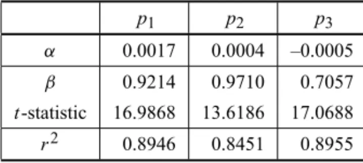
The results of an estimation of the parameters of regression between the nominal returns of the calculated portfolios and the market index returns are shown in Table 6.
Table 6– Estimated parameters and regression analysis statistics.
p1 p2 p3
α 0.0017 0.0004 –0.0005
β 0.9214 0.9710 0.7057
t-statistic 16.9868 13.6186 17.0688
r2 0.8946 0.8451 0.8955
Source: Elaborated by the author.
coefficients of 0.04% and –0.05% respectively; in the case of the maximum entropy model, the portfolio presented a monthly average loss of 0.05% irrespective of the market.
In terms of the Beta coefficient(β), the classic Markowitz and relative minimum entropy models presented risk levels that were very close to the market risks, the parameters of which were estimated with a high statistical significance. In these circumstances, it is envisaged that for each 1% variance in the market index returns, there will be a variance of 0.9214% in the returns for the portfolios composed according to the Markowitz model and nearly 0.9710% in returns for the portfolios composed according to the relative minimum entropy model. However, the maximum entropy model presented a moderate level of market risk, the returns of which followed a 0.7057% movement of 1.0% in the market index returns.
Some authors stated that the coefficient of determination(r2)can be considered as a measure of the diversification of the portfolio, since it measures to what degree the return variance of a portfolio is explained by the variability of the market index returns. If this is effectively taken into account, all the proposed portfolios in this study would have had a high level of diversification, since over 80.0% of their variabilities followed market movements.
However, the coefficient of determination may be questioned as a measure of diversification, since the market indices are composed of a very small number of companies in comparison with the stock market as a whole and by the fact that, in situations of crisis, there is a greater tendency for the movement of the majority of assets to follow the market, which could justify the high coefficients obtained during the period analyzed.
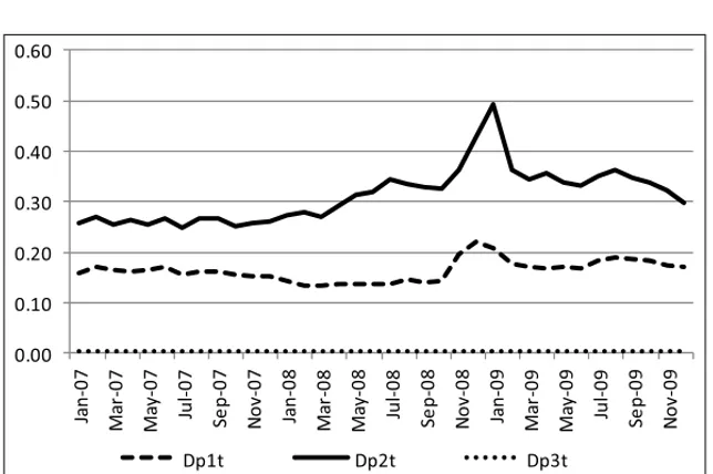
3.3.4 An analysis of the degree of portfolio diversification
The methodology used to measure the level of portfolio diversification as proposed by Goetz-mann & Kumar (2001), the results of which may be seen in Table 7 and Figure 3, show that the maximum entropy model presented the greatest level of diversification, with an average index of 0.0042; that is to say, very close to the maximum level of diversification.
Table 7– Average indices of portfolio diversification.
D p1 p2 p3
Mean 0.1636 0.3121 0.0042
σ 0.0209 0.0532 0.0003
Source: Elaborated by the author.
Figure 3– Monthly indices for portfolio diversification. Source: Elaborated by the author.
An explanation for this situation is found within the ambit of restrictions to which the entropic optimization models were submitted. While the maximum entropy model was only conditioned to the total weight vector unit and by the non-negativity of weights, the minimum relative entropy was, additionally, required to present a required level of desired return.
4 FINAL CONSIDERATIONS AND RECOMMENDATIONS
Even though more than fifty years have elapsed since the creation of the Modern Portfolio Theory, the fundamental characteristics of the classic Markowitz model can still be used to test the world’s new economic configurations and produce good results.
When comparing the Markowitz model with two models that were constructed to represent new risk configurations based on entropy optimization, the present study concluded that the first model was far superior to the others. Not only did the Markowitz model present better accu-mulated nominal yields, it also presented a far greater predictive efficiency and better effective performance, when considering thetrade-off between risk and return.
minimum entropy model presented an even lower degree of diversification than the Markowitz model. For instance, during one month in particular, this model managed to concentrate nearly 74.0% of its weights in only one asset. This unexpected behaviour in the entropic model can be explained by the restrictions imposed by the desired performance that is established in its formulation. For this reason, the model needed to respect this condition, thereby sacrificing its objective function performance.
Contrary to these two models, the maximum entropy model showed a level of diversification that was very close to the maximum level, which would be a situation that is far more in keeping with Markowitz’s diversification precepts. However, these models showed the worst results in the comparative analysis of performance.
It is important to underline that the results of these studies need to be interpreted in the light of the temporal context in which they are based and on the limitations of the IBOVESPA as an index representing the Brazilian stock market.
Further studies may be developed to find ways to study other periods to analyze, other markets, other market indices and to include other types of financial assets. In addition, new studies could consider the question of rebalancing portfolios over longer (annual) and shorter periods. In the latter case, the effects of intraday trading can also be studied, on condition that these took into account transaction costs. Other research studies could also compare the models used in this
study with downside risk models and of multiple periods, these last to be based on dynamic
programming.
REFERENCES
[1] BAWA V. 1982. Stochastic Dominance: A Research Bibliography. Management Science, 28(6): 698–712.
[2] BERAAK & PARKSY. 2008. Optimal Portfolio Diversification Using the Maximum Entropy Prin-ciple.Econometric Reviews,27(4-6): 484–512.
[3] BMFBOVESPA – BOLSA DE MERCADORIAS & FUTUROS E BOLSA DE VALORES DE S ˜AO
PAULO. 2010. Cotac¸˜oes hist´oricas. Dispon´ıvel em:
http://www.bmfbovespa.com.br/shared/iframe.aspx?idioma=pt-br
&url=http://www.bmfbovespa.com.br/pt-br/cotacoes-historicas/FormSeriesHistoricas.asp.
[4] CASSETTARIA. 2003. O Princ´ıpio da M´axima Entropia e a Teoria das Carteiras.Revista Brasileira de Financ¸as,1(2): 271–300.
[5] GOETZMANNWN & KUMARA. 2001. Equity Portfolio Diversification.NBER Working Paper 8696, National Bureau of Economic Research, Cambridge. Dispon´ıvel em:
http://web.econ.unito.it/nicodano/w8686.pdf.
[6] HUA L & XINGSI L. 2003. A New Portfolio Model and Application. Operations Research and Management Science,6: 83–86.
[8] KWAN CCY. 2001. Portfolio Analysis Using Spreadsheet Tools.Journal of Applied Finance, 11: 70–81.
[9] MARKOWITZHM. 1952. Portfolio Selection.The Journal of Finance,7(1): 77–91.
[10] MARKOWITZHM. 1959.Portfolio Selection, Efficient Diversification of Investments.New Jersey: John Wiley & Sons.
[11] MARKOWITZ HM. 1987.Mean-Variance analysis and portfolio choice and capital market. New York: John Wiley & Sons.
[12] OGRYCZAK W & RUSZCZYNSKI A. 1999. From stochastic dominance to mean-risk models: Semideviations as risk measures.European Journal of Operational Research,116(1): 33–50.
[13] PHILIPPATOSGC & WILSONCJ. 1972. Entropy, market risk, and the selection of efficient portfolios. Applied Economics,4: 209–220.
[14] PHILIPPATOSGC & WILSONCJ. 1974. Entropy, market risk, and the selection of efficient portfolios: Reply.Applied Economics,6: 77–81.
[15] R ¨ODDERW. 2000. Conditional logic and the Principle of Entropy.Artificial Intelligence,117: 83– 106.
[16] RUBINSTEINM. 2002. Markowitz’s “Portfolio Selection: A Fifty-Year Retrospective”.The Journal of Finance,57(3): 1041–1045.
[17] SHARPEWF. 1963. A simplified model for portfolio analysis.Management Science,9(2): 277–293. [18] SHARPEWF. 1964. Capital Asset Prices: A theory of Market Equilibrium under Conditions of Risk.
The Journal of Finance,19(3): 425–442.
[19] SHARPEWF. 1966. Mutual Fund Performance.The Journal of Business,39(1), Part 2: Supplement on Security Prices, 119–138.
[20] SHANNONCE. 1948. A Mathematical Theory of Communication.The Bell System Technical Jour-nal,27: 379–423.
[21] STEINBACHMC. 2001. Markowitz Revisited: Mean-Variance Models in Financial Portfolio Analy-sis.Society for Industrial and Applied Mathematics,43(1): 31–85.