UNIVERSIDADE DA BEIRA INTERIOR
Ciências Sociais e Humanas
Delinquency and default in the USA student debt
as fractional response to unemployment and
average debt per borrower
Estefano da Rocha Oliveira da Silva
Dissertação para obtenção do Grau de Mestre em
Economia
(2º ciclo de estudos)
Orientador: Prof. José Alberto Serra Ferreira Rodrigues Fuinhas
iii
Agradecimentos
Esta dissertação não podia ter sido possível sem o apoio de muitas pessoas a quem tenho de expressar a minha gratidão.
Em primeiro lugar, devo agradecer aos meus pais, à minha irmã e restantes familiares por todo o carinho, compreensão e todo o apoio nesta minha aventura académica.
Um obrigado muito especial também à minha namorada Elisa, que apesar da distância, sempre me apoiou e ajudou nesta jornada da minha vida com muito amor e carinho.
Em seguida, expresso a minha gratidão ao meu orientador, Professor José Alberto Serras Ferreira Rodrigues Fuinhas, que se mostrou sempre disponível e acessível a mim e aos meus colegas, para que um estudo interessante pudesse ser realizado. A sua ajuda e sugestões contribuíram para um melhor trabalho.
Por último, um agradecimento especial a todos as amizades que fiz na Universidade da Beira Interior, que me apoiaram e serviram como uma segunda família neste meu percurso, com momentos que com certeza deixarão saudades.
v
Resumo
A dívida dos estudantes e o seu default têm sido um tema popular de estudo nas últimas décadas, sendo a maioria destes estudos feitos nos EUA. Nesta investigação, estudamos a resposta da proporção de estudantes que pediram empréstimos com créditos malparados a mais de noventa dias ou em default para variáveis como desemprego e a dívida média por estudante que contraiu empréstimo, nos Estados Unidos, usando dados em painel de 50 estados, entre 2004 e 2012. Esta proporção de estudantes com créditos malparados ou em default está modelado como respostas fracionarias para o desemprego, dívida média por estudante que contraiu empréstimo, sentimento do consumidor e stress financeiro. Por isso, o probit fracionário é usado como modelo econométrico, que especifica meios condicionais de efeitos não observados do estado e do ano, como funções lineares das covariáveis. Os testes de especificação indicam normalidade, ausência de autocorrelação e homocedasticidade, e nenhuma variável relevante é omitida. Desemprego e dívida média por estudante são estatisticamente significativas e contribuem para o aumento de crédito malparado ou o
default.
Palavras-chave
Default dos empréstimos de estudantes; desemprego; dívida média por estudante; sentimento
vii
Resumo Alargado
A dívida dos estudantes e default nos empréstimos têm sido um tema popular de estudo nas últimas décadas, sendo a maioria destes estudos feitos nos EUA, em que a dívida dos estudantes é a segunda maior dívida dos consumidores no país, depois das hipotecas e maior que a dívida de cartões de crédito e empréstimos para carros. Nesta investigação, o objetivo é estudar a reação dos níveis de incumprimento dos empréstimos estudantis tendo em conta determinantes como o desemprego e a dívida média por estudante que contraiu empréstimo, nos Estados Unidos, usando dados em painel de 50 estados, entre 2004 e 2012. A nossa hipótese primária é que quanto maior o desemprego e montante de dívida média por estudante com empréstimo maior é a proporção de crédito malparado ou default.
O estudo centra-se nos EUA por ser o país com maior informação e dados disponíveis comparativamente a países que têm um sistema de ensino superior semelhante como por exemplo, o australiano e o inglês, que sofrem do mesmo problema que o americano em relação aos empréstimos, mas que têm uma escassez de dados sobre o assunto. O período de estudo foi escolhido por ter sido o mais recente e com maior número de anos possível, mas que inclui o período de recessão causado pela crise financeira de 2007-2008.
Na literatura relacionada com o tema é revelado que uma considerável percentagem de estudantes opta por áreas de estudo que lhe permitirão enveredar em carreiras com melhores salários (Herr and Burt, 2005) e estudantes com empréstimo que já estiveram desempregadas têm uma probabilidade maior de default do que outros que não passaram pelo desemprego (Woo, 2002).
O crescimento da percentagem de default é em parte associada a estudantes com empréstimos provenientes de escolas com fins lucrativos (Goodell, 2016; Looney and Yanellis, 2015), onde as propinas são mais altas que outro tipo de instituições e continuam a subir, contribuindo para um aumento do valor emprestado aos estudantes (Cellini and Darolia, 2015). Os estudantes destas instituições também acabam com maiores taxas de desemprego comparado com outro tipo de instituições (Deming et al., 2012).
Estudantes que completam os seus estudos têm menor probabilidade de default do que estudantes que não completam o plano de estudos (Podgursky et al., 2002). Outros estudos, sugerem que à medida que a carga da dívida aumenta, aumentam também as probabilidades de default (Choy and Li, 2006; Lochner and Monge-Maranjo, 2004; Dynarski, 1994). O risco de
viii
trabalho com carreiras de rendimento baixo (Woo, 2002). Se a dívida mensal ultrapassar 8% do rendimento, a dívida do empréstimo é considerada incontrolável (Choy and Li, 2006).
Esta investigação utiliza dados em painel, com 450 observações e todas as variáveis independentes encontram-se na forma de logaritmo natural. Como variável dependente temos a proporção de estudantes que pediram empréstimos com créditos malparados a mais de noventa dias ou em default, da Reserva Federal de Nova Iorque e a Equifax. Também da mesma base de dados, mas como variável independente, temos a dívida média por estudante que contraiu empréstimo. Outra variável independente é a taxa de desemprego que tem como fonte a US Bureau of Labor Statistics. As outras duas variáveis independentes utilizadas são o Índice do sentimento do consumidor da Universidade do Michigan e o Índice de stress financeiro de St. Louis, ambas as variáveis da Federal Reserve Economic Data. Estas duas últimas variáveis são a nível federal e não estadual.
Para uma boa estimação num painel, recorremos a testes e diagnósticos especificamente para dados em painel. Estes indicaram para a existência de normalidade, ausência de autocorrelação e homocedasticidade, a não existência de multicolinearidade, e nenhuma variável relevante é omitida.
A variável dependente neste estudo é limitada entre 0 e 1. Papke e Wooldridge (2008) defendem que para este caso de dados em painel, como é o nosso caso, seria aplicar o probit fracionário.
Este modelo introduzido por Papke e Wooldridge (2008) pode ser aplicado para estimar modelos de resposta fracionaria para dados em painel com grande dimensão e poucos períodos de tempo que permite que efeitos temporais constantes não observados, serem correlacionados com as variáveis explicativas. Os dados não precisam de envolver toda a população, mas requerem um conjunto de dados em painel balanceado com toda a informação sobre as variáveis em cada ano para cada estado. Para fins de comparação, também foi usado um modelo linear e apresentamos os resultados juntamente com o probit fracionário, com erros robustos e bootstrapped.
Os resultados mostram que desemprego, dívida média por estudante que contraiu empréstimo e o sentimento do consumidor têm um impacto positivo e estatisticamente significativo na proporção de estudantes que pediram empréstimos com créditos malparados a mais de noventa dias ou em default, em ambos os modelos, linear e probit fracionário. O stress financeiro é não estatisticamente significativo, em qualquer dos modelos. Assim, aceita-se a hipótese primária, em que maior desemprego e montante na dívida média por estudante com empréstimo irá levar a uma maior proporção de crédito malparado ou default.
Uma comparação entre as estimativas do modelo linear e os efeitos marginais do probit fracionário indica que sua ordem de grandeza é muito semelhante e que as diferenças nas estimativas dos parâmetros são relativamente consideráveis.
ix
A relação positiva entre a taxa de desemprego e a proporção de estudantes que pediram empréstimos com créditos malparados a mais de noventa dias ou em default, pode ocorrer por causa de estudantes que optam por cursos que têm altos níveis de desemprego, de alunos de instituições com fins lucrativos e pessoas no desemprego sem poupanças para fazerem pagamentos das mensalidades do empréstimo.
O impacto positivo da dívida média por estudante na proporção de estudantes que pediram empréstimos com créditos malparados a mais de noventa dias ou em default pode dever-se ao aumento das propinas ao longo dos anos e ao facto de estudantes enveredarem por carreiras de salários baixos, que irão estar envolvidos em maiores dificuldades no pagamento dos seus empréstimos.
Podem ser tomadas algumas medidas para diminuir esta proporção de crédito malparado e default, como fazer com que credores peçam um maior pagamento de juros a estudantes que representem um maior risco de default. Também podem ser limitados o número de vagas para cursos com altos níveis de desemprego. Outra alternativa poderia ser, o governo mudar o seu sistema de ensino superior para um similar a países europeus, onde as propinas são pagas parcialmente ou totalmente pelo estado. Estas medidas poderiam ter um efeito significativo na redução desta proporção.
Este estudo é o primeiro a usar um modelo probit fracionário para dados em painel para a análise da proporção de estudantes com crédito malparado ou em default. Os estudos existentes sobre o default de estudantes nos EUA utilizam dados de uma universidade ou região em específico. Neste estudo utilizamos dados de 50 estados.
xi
Abstract
Student debt and default has been a hot topic of research in the last decades, being majority of these studies done in the USA. In this paper we study the response of the proportion of student borrowers with ninety or more days of delinquency or in default to variables such as unemployment and the average debt per borrower, in the United States, using a panel data of 50 states, from 2004 to 2012. The proportion of borrowers with delinquency or default are modeled as fractional responses to unemployment, average debt per borrower, consumer sentiment and financial stress. Therefore, a fractional probit is used as econometric model, which specifies conditional means of state and year unobserved effects, as linear functions of the covariates. The specification tests indicate normality, absence of autocorrelation and homoscedasticity, and supports that no relevant variable was omitted. Unemployment, and the average debt per borrower are statistically significant and contributes to increase the delinquency or default in the USA.
Keywords
Student loan default; unemployment; average debt per borrower; consumer sentiment; financial stress; fractional probit; panel data.
xiii
Contents
1 Introduction 1
2 Literature review 3
2.1 Student characteristics and default 3 2.2 Institutional characteristics and default 4
2.3 Enrollment and default 4
2.4 Income and default 5
2.5 Unemployment, debt and default 5
3 Methodology 9
4 Data 13
5 Tests and diagnostics for panel data 17
5.1 Distribution of model errors 17
5.2 Correlation of model errors 17
5.3Omitted and redundant Variable Bias 18
5.4 Multicollinearity 18
5.5 Random vs fixed effects model 19
6 Empirical results 21
7 Discussion 25
8 Conclusion 27
xv
List of figures
Figure 1 - Representation of default and its causes according to previous literature 6 Figure 2 - Proportion of student loan borrowers on ninety or more days delinquency
or default, 2004-2012
15 Figure 3 - Natural log of unemployment rate, 2004-2012 15 Figure 4 - Natural log of the average debt per borrower, 2004-2012 16 Figure 5: Representation of a possible response of the proportion of student
borrowers with the different independent variables
xvii
List of tables
Table 1 - Description, acronym and source of the variables 14
Table 2 - Descriptive statistics 14
Table 3 - Breusch-Pagan and Doornik-Hansen Tests 17 Table 4 - Pesaran and Wooldridge Tests 17
Table 5 - Ramsey Test 18
Table 6 - VIF 18
Table 7 - Breusch-Pagan test for random effects 19 Table 8 - Estimated results with robust standard errors 21 Table 9 - Estimated results with bootstrapped standard errors 23
xix
List of acronyms
GEE Generalized Estimating Equation GLM Generalized Linear Models
STEM Science, technology, engineering and mathematic Probit Probability Unit
AR(1) Autoregressive model of order 1 VIF Variance inflation factors
xx
1
1. Introduction
Student Loan debt is becoming a huge concern for the US economy. It is the second highest consumer debt, after mortgages and higher than credit card and auto loans debt. Students debt was around $1.3 trillion at the end of 2016, an increase of 170% since 2006. Reasons for this increase are: more student taking loans, with larger amounts and repayment rates have slowed down. The aim of this paper is to study the response of the proportion of USA student borrowers with ninety or more days delinquency or in default to variables such as unemployment and average debt per borrower at a state level, being the first use of a fractional probit model for panel data for student borrower delinquency or default data analysis. Our primary hypothesis in this paper is that higher unemployment and average debt per borrower will lead to a higher proportion of student borrowers’ delinquency or default.
Around 5% of the borrowers have more than $100.000 in debt but represent 30% of total debt. The recent graduates leave the education institution on average with about $34000 in student debt. Default rates have increased until 2012 and is stabilized since 2013. Payment progress is slower for more recent graduates because of higher borrowing amounts and higher default rates (Chakrabarti et al., 2017).
The risk of student loan default can be a potential trigger for the next financial crisis, since the 30+ days delinquency rate increased between 2004 and 2014, from 11 percent to 17%, much higher than other kind of debt (Sánchez and Zhu, 2015).
College enrollment grew by 20% between 2005 and 2010, faster than any period since the 1970s and has been declining since (Haughwout et al., 2015), with an increase in the student loan borrowing during the Great Recession (2007-2012) and doubled in real terms between 2005 and 2012. This increase was probably driven from higher tuition and college costs.
Constrained family finances and weak labor markets, after the recession, could also be a reason for students to attend graduate and professional schools. High loan debt might not be a problem if the investment has high returns in the future and repayments are made (Naranjo, 2014). Some institutions have price discrimination which allows to benefit student from low income families, being education a bigger burden for students of wealthier families (Wolla, 2014).
Most students in repayment says that the benefits of education made possible through borrowing are well worth any problem associated with paying off the loans. But there is also indication of negative attitudes against education debt, which are increasing. Borrowers of low
2
income families have bigger probability to have problem with repayments (Baum and O’Malley, 2003).
College is on average, a better investment today than a generation ago, but there is a probability of having large, small or even negative return. Student from community colleges have low completion rates and are unlikely to have substantial earning associated with degree completion. For-profit institutions students, with weak incomes are usually connected with elevated levels of borrowing, making them more usually to default on loans (Avery and Turner, 2012).
Degree completion increases the amount of debt the as the amount of borrowing increases, meaning that borrower with high debt completed either associate or bachelor degree than those with low debt. Default can have originated from different causes, like individuals with low debt maybe have difficulties repaying their loan in recent years because of the slow labor market conditions with less than a bachelor degree. Those with a bachelor degree entered better labor markets, but still not good enough sometimes to repay their high debt. The most serious cases are the ones with high debt and no advanced degree (Naranjo, 2014).
The remainder of the paper is organized as follows: next section provides a Literature review on proportion of students with loan default. Section 3 present the Methodology, followed by section 4 with the Data. Section 5 presents the Tests and diagnostics for panel data and section 6 reports the Empirical results. Section 7 disclosures the Discussion. And section 8 concludes.
3
2. Literature review
Nearly all the existing literature on student loan default are focused on the United States where student loan is a prominent issue for higher education and the second most substantial consumer debt in the country.
One of studies outside the US by Han et al. (2015) made in South Korea, analyzes factors affecting default on student loans, concluding that default is function of gender, major and loan amount, also documenting new variables that are affecting default such as grace period and repayment period.
2.1 Student characteristics and default
Literature about the US reveal program completion, persistence and success were strong predictors of student loan default just like were race or ethnicity, gender and the type of school enrollment in University. Role of the student success and graduation indicate that are substantial in eventual loan repayment (Herr and Burt, 2005).
Debt makes graduates choose higher salary jobs and reduce the choice on low paid public interest jobs and college students are also not life cycle agents, because they are credit constrained and averse to holding debt, which can eventually reduce student donations to the former institutions (Rothstein and Rouse, 2011).
Poor academic performance is the main reason for student departure, and departure before completing the degree is one of the reasons for loan default (Volkwein and Cabrera, 1998) and the number of hours failed in university by student borrowers also increase the chances of default (Steiner and Teszler, 2003; Christman, 2000).
Families of students whose parents had higher levels of education were less likely to default than first generation university students (Choy and Li, 2006; Volkweing et al., 1998, Volwein and Szelest, 1995) and other studies also found that male and older students increase the borrower’s chance to default (Woo, 2002; Podgursky et al., 2002; Flint, 1997). Researchers have been remarkably consistent on the conclusion that student of color are more likely to default than Caucasian students (Harrast, 2004; Woo, 2002; Christman, 2000; Volkwein and Cabrera, 1998; Volkwein and Szelest, 1995;).
4
When it comes to compare non-financially at-risk students with financially at-risk students, the later ones have much higher student loan balances and usually prioritize their credit card bills before repaying their student loans (Pinto and Mansfield, 2006) and a study by Woo (2002) reveals that borrowers who were into delinquency more than one time are more likely to end up defaulting.
Students who obtain information indicating that might not be able to repay their loans are more likely to change to higher earning majors, with higher academic results students choosing in preference science, technology, engineering and mathematic (STEM) fields (Schemeiser et al., 2016).
2.2 Institutional characteristics and default
When examining the relation between institutional characteristics and student loan default, there can be found significant differences such as admission yield, geographic region, percentage of minority students, private or public institution, endowment and expenditures for student services (Webber and Rogers, 2014).
Most increment in default are associated with borrowers from for-profit schools, two-year institutions and nonselective institutions. These students only represent a small share in all student borrowers. The majority come from low income families, attended institutions with poor educational outcomes and facing weak labor markets outcomes after leaving the educational institutions. When it comes to borrowers who attended most four-year public and nonprofit private institutions, default rates remained low, which represent the larger part of the federal loan portfolio. Higher earnings, low unemployment rates and better family resources appear to have helped this category of borrowers during tough times (Looney and Yanellis, 2015).
2.3 Enrollment and default
Continuous enrollment can be also associated with student loan default. Borrowers that withdraw from university for whatever reason have higher default rates, with the rates rising at the same time as the number of withdrawn rises, being the default rates higher for students who withdraw for administrative or academic reasons than students who withdraw for work-related reasons (Steiner and Teszler, 2003).
In a time range from four to eight semesters, students who are continually enrolled or complete their program are less likely to default than are students who dropout during the same period (Podgursky et al., 2002). Learning ability and initial stock of human capital combined has influence on the decision to enroll in college, and parental wealth has minimum minimal effects and increases enrollment with repayment flexibility (Ionescu, 2009).
5
2.4 Income level and default
Ionescu and Simpson (2016) observed borrowing default behavior across family income and student preparation and found out that more government borrowing limits increase college investment and lead to more default in student loans’ private market, and tuition subsidies increase college investment and reduce default rates.
Knap and Seaks (1992) found that chances of default decrease when the borrower has two parents and a high income. But when it comes to family assets, net worth from households without an outstanding student loan is almost three times higher than households with outstanding student debt. Households with outstanding student loan debt incur in a lost around 54% of the net worth compared with households with similar net worth levels but without student loans in the same period (Elliot and Nam, 2013).
Credit constraints possibly play an important role in the drop-out decision in some students, but to the majority of students from low income should be attributed reasons besides credit constraints (Stinebrickner and Stinebrickner, 2008). Without surprise, borrowers with high earnings after they leave school are less likely to default than those with low earnings. This fact highlights the risk that students assume when taking out large loans and then entering in a labor market with low-paying careers. And also, borrowers who went into delinquency more than once are more likely to default (Woo, 2002). Student debt is also negatively related to the predisposition to start a firm, in particular larger and successful ventures (Krishnan and Wang, 2018).
2.5 Unemployment, debt and default
Our objective in this investigation is to study the response of student borrowers towards unemployment and the average debt per borrower. Previous literature reveals that borrowers who experienced unemployment showed an increase in their probability of default over their original probability and also borrowers whose loan are held by more than one provider were more likely to default, with each additional provider increasing the odds of default by 18 percent. And the number of loans, but not the amount borrowed, is related to default, with more loans signaling a higher risk (Woo, 2002). Students from for-profit Institutions also end up with higher unemployment rates (Deming et al., 2012).
Literature about the amount of debt suggests that as the debt burden increases so does the odds of default. The average debt burden may differ by the type of institution, but whatever the type of institution, the more a student borrows the greater is the odds of default (Choy and Li, 2006; Lochner and Monge-Maranjo, 2004; Dynarski, 1994).
If the monthly debt burden outpaces 8 percent of income, the loan debt is considered unmanageable. Choy and Li (2006) acclaimed that 11 percent of borrowers proclaimed
6
unmanageable debt levels by 2003, with more than 20 percent of these students ending up defaulting. But there can be found an exception respecting to high debt and odds of default, which are the students who incurred in high levels of debt by attending graduate school which were less likely on average to default (Woo, 2002; Volkwein et al., 1998).
High and rising tuition, but relatively low student financial resources in the for-profit sector are likely the key factors contributing to increased borrowing in the for-profit sector (Cellini and Darolia, 2015). For-profit institutions systematically encourage ill-advised loans. The results are economically significant, with default rates generally 5 to 6 percentage points higher in for-profit institutions (Goodell, 2016). An increase of credit limits and expansions in credit availability resulted in increasing the borrowing amount by students (Looney and Yannelis, 2018).
This literature helps to complement this investigation when it comes to determine why unemployment and the average debt per borrower affect the proportion of student borrowers with ninety or more days delinquency or in default.
Figure 1 represents default and its causes according to the previous literature.
Figure 1: Representation of default and its causes according to previous literature
Default Gender Major High loan amount Race or ethnicity Poor academic performance Not completing study program Hours failed Age Delinquency Low income careers Individual/family income Unemployment For-profit institutions Increasing tuitions
7
This figure shows the main causes of default by different authors in the previous literature over the last decades from different universities and regions in the USA. It includes unemployment and the loan amounts, key factors for this study, and others like the for-profit institutions and increasing tuitions over the years. As the figure demonstrates, there is a several number of causes for the increase of default among student borrowers, with some having more impact than others.
9
3. Methodology
In this study, we estimate our model using a generalized estimating equation (GEE). The GEE incorporates many models such as: logistic and probit regression, ordinary least squares, ordinal outcome regression, regression models for the analysis of survival data, and other models (Liang and Zeger, 1986).
The GEE is a generalization of the generalized linear models (GLM) but that considers the within-group correlation, since the GLM Is inadequate when data are longitudinal or are otherwise grouped so that the observation within the same group are expected to be correlated (Hardin and Hilbe, 2013).
Since GEE fits generalized linear models of
𝑦
𝑖𝑡 with covariates𝑥
𝑖𝑡 in equation (1)𝑔{𝐸(𝑦
𝑖𝑡)} = 𝑥
𝑖𝑡𝛽, 𝑦 ~ 𝐹 𝑤𝑖𝑡ℎ 𝑝𝑎𝑟𝑎𝑚𝑒𝑡𝑒𝑟𝑠 𝜃
𝑖𝑡 (1)for
𝑖 = 1, … , 𝑚
and𝑡 = 1, … , 𝑛
𝑖 where𝑛
𝑖 is the number of observations for each group identifier𝑖
.𝑔
is called the link function, and𝐹
is the distributional family. The different definition for𝑔
and𝐹
result in a wide bundle of models. For example, if𝑔
is the probit function and𝑦
𝑖𝑡 is distributed Bernoulli (binomial), we have equation (2)𝑝𝑟𝑜𝑏𝑖𝑡{𝐸(𝑦
𝑖𝑡)} = 𝑥
𝑖𝑡𝛽, 𝑦 ~𝐵𝑒𝑟𝑛𝑜𝑢𝑙𝑙𝑖.
(2)Calling
𝑅
the working correlation matrix for modelling the within-group.𝑅
𝑡,𝑠 stand for the𝑡, 𝑠
element in the correlation structures.The independent structure is defined as equation (3)
𝑅
𝑡,𝑠= {
0 𝑜𝑡ℎ𝑒𝑟𝑤𝑖𝑠𝑒
1 𝑖𝑓 𝑡 = 𝑠
(3)
The exchangeable structure, comparable to equal-correlation models, is defined as equation (4)
𝑅
𝑡,𝑠= {
1 𝑖𝑓 𝑡 = 𝑠
𝜌 𝑜𝑡ℎ𝑒𝑟𝑤𝑖𝑠𝑒
10
The ar1 structure is defined for correlation of an AR(1) model, given by equation (5)
𝑅
𝑡,𝑠= {
1 𝑖𝑓 𝑡 = 𝑠
𝜌
|𝑡−𝑠|𝑜𝑡ℎ𝑒𝑟𝑤𝑖𝑠𝑒
(5)
The stationary 1 structure is given by equation (6)
𝑅
𝑡,𝑠= {
1 𝑖𝑓 𝑡 = 𝑠
𝜌 𝑖𝑓 |𝑡 − 𝑠| = 1
0 𝑜𝑡ℎ𝑒𝑟𝑤𝑖𝑠𝑒
(6)
And unstructured structure appoints only the constraint that the diagonal elements of working correlation matrix be 1, in equation (7)
𝑅
𝑡,𝑠= {
1 𝑖𝑓 𝑡 = 𝑠
𝜌
𝑡𝑠𝑜𝑡ℎ𝑒𝑟𝑤𝑖𝑠𝑒, 𝜌
𝑡𝑠= 𝜌
𝑠𝑡(7)
The values of our dependent variable are bounded between 0 (no borrower is ninety or more days delinquent or in default) and 1 (every borrower is ninety or more days delinquent or in default). Papke and Wooldridge (2008) defend for that case of panel data, as it is in our case, the fractional probit is better suited, and it’s the method used in this paper.
This model introduced by Papke and Wooldridge (2008) can be applied to estimate fractional response models for panel data with large cross-sectional dimension and relatively few time periods while allowing for time constant unobserved effects, that can be correlated with explanatory variables. The data need not to involve the whole population, but it must be a balanced panel data set with the entire information on all variables in each year for each state.
Using a Generalized Estimating Equation on Stata 14, we estimate the model specifying a probit link function, a Bernoulli distribution and an exchangeable correlation matrix, using robust standard errors (table 8) and 500-bootstrap iteration to calculate standard errors (table 9). Such model allows to account the presence of serial correlation and heteroskedasticity.
This give us the following model, equation (8):
𝐸(𝑦
𝑖𝑡|𝑥
𝑖𝑡, 𝑐
𝑖) = Φ(𝑥
𝑖𝑡𝛽 + 𝑐
𝑖)
(8)where
𝑖
represents clusters,𝑡
represent the year andΦ
the standard cumulative distribution function. The dependent variable,𝑦
𝑖𝑡, represent the proportion of borrowers who are ninety or more days delinquent or in default, where0 ≤ 𝑦
𝑖𝑡≤ 1
. The𝑥
𝑖𝑡 is the set of explanatory variables,𝑐
𝑖 stands for the unobserved effects possibly correlated with the explanatory variables.Concerning to the modeling of
𝑐
𝑖, we adopt the Mundlak-Chamberlain-Wooldridge device (see Mundlak, 1978, Chamberlain, 1982, 1984 and Wooldridge, 2002) like Papke and Woolridge (2008) and consider that𝑐
𝑖 is normally distributed on𝑥
𝑖𝑡, defined as equation (9)11
𝑐
𝑖= 𝜓 + 𝑥̅
𝑖𝜉 + 𝑎
𝑖,
𝑎
𝑖|𝑥̅
𝑖~𝑁𝑜𝑟𝑚𝑎𝑙(0, 𝜎
𝑎)
(9)where
𝑥̅
𝑖≡ 𝑇
−1∑
𝑇𝑡=1𝑥
𝑖𝑡 is a column vector of the time averaged explanatory variables for state𝑖
and𝜎
𝑎 is the conditional variance of𝑐
𝑖. Writing this expression into (8), we get equations (10) and (11)𝐸(𝑦
𝑖𝑡|𝑥
𝑖𝑡, 𝑐
𝑖) = Φ(𝜓 + 𝑥
𝑖𝑡𝛽 + 𝑥̅
𝑖𝜉/(1 + 𝜎
𝑎)
1/2)
(10)𝐸(𝑦
𝑖𝑡|𝑥
𝑖𝑡, 𝑐
𝑖) = 𝜓
𝑎+ 𝑥
𝑖𝑡𝛽
𝑎+ 𝑥̅
𝑖𝜉
𝑎 (11)and see that
𝛽
is identified to the positive scalar(1 + 𝜎
𝑎)
1/2(see Papke and Wooldridge, 2008).The parameters
𝜓
𝑎,𝛽
𝑎 and𝜉
𝑎 are consistently estimated when applying a Pooled (fractional) probit analysis, also called Population average probit for fractional responses, by using the GEE (Generalised Estimating Equation) method.For comparison purposes, we will also use a linear model and present results together with the fractional probit. This allows us to compare the gain obtained from a proper treatment of the proportion of delinquents and defaulters as fractional responses.
Panel data models are often estimated with linear models, with either fixed effects or random effects models. Random effects models make the presumption that random effects are uncorrelated with the random error. When this presumption is wrong, the random effects estimator will be conflicting (Greene, 2002). As random effects are a more adequate estimator than fixed effects, we should use random effects if it is statistically possible.
The random effects equation is defined as in equation (12):
𝑦
𝑖𝑡= 𝛽𝑥
𝑖𝑡+ 𝛼 + 𝑢
𝑖𝑡+ 𝜀
𝑖𝑡 (12)where
𝑦
is our dependent variable, the proportion of student borrowers who are in delinquency or default,𝑖
represents states and𝑡
stands for time,𝑥
is the matrix of independent variables,𝛽
is the coefficient for the independent variables,𝛼
is the unknown intercept for each state,𝑢
is the between-state error and𝜀
is the within-state error.And the fixed effects equation is defined as in equation (13):
𝑦
𝑖𝑡= 𝛽𝑥
𝑖𝑡+ 𝛼
𝑖+ 𝑢
𝑖𝑡 (13)where
𝑦
is our dependent variable,𝑖
represents states and𝑡
the years,𝑥
is the matrix of independent variables,𝛽
is the coefficient for the independent variable,𝛼
𝑖 is the unknown intercept for each state and𝑢
𝑖𝑡 is the error term.A test will be used later in this investigation to determine whether to use a random or fixed effects model.
13
4. Data
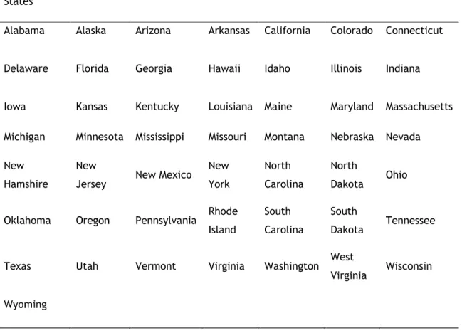
In this research, we are using a balanced annual panel data with the 50 states of the USA, from 2004 to 2012, with 450 observations and all the independent variables are in the form of natural logs.
This study focuses on the USA because there is more information and data compared to countries that have an identical higher education system like for example, the Australian and the English, that also suffer from the same problem in student loan default like the American but has a shortage of data on the subject. The period of study chosen was the most recent available and with most years possible but includes a period of recession caused by the financial crisis in 2007-2008.
As dependent variable we have the proportion of student loan borrowers with ninety or more days past due accounts including defaults by state (def), from the Federal Reserve Bank of New York and Equifax. The data was created from a 1% sample of US population with credit information and includes both federal student loans and private student loans.
As independent variables we use the average student debt balance per borrower (ln(adb)) by state also from the FRBNY and Equifax, from the 1% sample with credit information and including both federal and private student loans.
Another variable is the unemployment rate (ln(unem)) by state, with the US Bureau of Labor Statistics as source.
The last two variables are the University of Michigan: Consumer Sentiment Index (ln(cs)) and the St. Louis Fed Financial Stress Index (ln(fstress)), both on a federal level because there is no information about this data by state and both from Federal Reserve Economic Data. The University of Michigan: Consumer Sentiment Index is a consumer confidence Index used as a statistical measurement and economic indicator of consumers attitudes about their financial position and present situation as well as the health of the economy in short and long term, published by the University of Michigan.
The St. Louis Fed Financial Stress Index measures financial stress in the markets and is constructed with 18 data series: seven interest rate series, six yield spreads and other five indicators with each one of them capturing some aspect of financial stress. As the level of financial stress in the economy changes, these data series are likely to move together. In this index, zero is viewed as representing normal financial market conditions, with values below
14
zero proposing a below-average financial market stress and values above zero proposing above-average financial market stress.
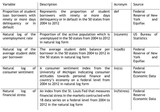
Table 1: Description, acronym and source of the variables
Variable Description Acronym Source
Proportion of student loan borrowers with ninety or more days delinquency or in default
Represents the proportion of student borrowers with ninety or more days delinquency or in default in the 50 states from 2004 to 2012
def Federal
Reserve of New
York and
Equifax
Natural log of the
unemployment rate Proportion of the active population which is unemployed in the 50 states from 2004 to 2012 in natural log form
ln(unem) US Bureau of
Statistics
Natural log of the average student debt per borrower
The average student debt balance per borrower in the 50 states from 2004 to 2012 in the 50 states in natural log form
ln(adb) Federal Reserve of New York and Equifax Natural log of consumer sentiment
A consumer sentiment index from the University of Michigan indicating consumer attitudes towards personal finance and country’s economy on a federal level from 2004 to 2012 in natural log form
ln(cs) Federal
Reserve Economic Data
Natural log of
financial stress
An index from the St. Louis Fed that measures financial stress in the markets contructed with 18 data series on a federal level from 2004 to 2012 in the natural log form
ln(fstress) Federal Reserve Economic Data
Table 2 shows the descriptive statistics on the proportion of borrowers who are ninety or more days delinquent or in default, and the explanatory variables in 50 states of the US. The average proportion of borrowers who are ninety or more days delinquent or in default is 8,1% between 2004 and 2012.
Table 2: Descriptive statistics
Variables Mean Std. Dev. Min Max Observations
def Overall .0810 .0249 .0320 .1780 N= 450 Between .0177 .0517 .1133 n= 50 Within .0176 .0220 .1492 T=9 ln(unem) Overall -2.823 .3548 -3.6497 -1.9805 N=450 Between .2091 -3.3790 -2.4326 n=50 Within .2880 -3.4853 -2.1854 T=9 ln(adb) Overall 9.8438 .1891 9.3326 10.2506 N=450 Between .0843 9.6405 10.0206 n=50 Within .1697 9.4917 10.1432 T=9 ln(cs) Overall 4.3479 .1384 4.1558 4.5560 N=450 Between 0 4.3479 4.3479 n=50 Within .1384 4.1558 4.5560 T=9 ln(fstress) Overall -0.2753 1.5593 -2.3026 1.6134 N=450 Between 0 -.2753 -.2753 n=50 Within 1.5593 -2.3026 1.6134 T=9
15
Figure 2 presents a graph with the progression of the proportion of student loan borrowers on ninety or more days delinquency or default in the 50 states from 2004-2012.
Figure 2: Proportion of student loan borrowers on ninety or more days delinquency or default, 2004-2012 Note: Own calculation - Graph generated by Stata
The proportion of students with delinquency or default started to rise in 2008 when the financial crisis began with lower levels in 2011 but rising its levels again in 2012.
Figure 3 represents the evolution of the natural log of unemployment rate in the 50 states from 2004 to 2012.
Figure 3: Natural log of unemployment rate, 2004-2012 Note: Own calculation - Graph generated by Stata
16
With the financial crisis, the unemployment rate started to grow noticing a significant disparity of the rate between 2008 and 2009 and decreasing slowly in the following years.
Figure 4 displays a graph with the expansion of the natural log of the average debt per student borrower in the 50 states from 2004 to 2012.
Figure 4: Natural log of the average debt per borrower, 2004-2012 Note: Own calculation - Graph generated by Stata
The amount of debt per borrower has been growing every year between 2004 and 2012. There were also some limitations in the data. We did not use variables like the cost of attendance in different types of institutions and the number of students with a loan because there were some missing observations making them not applicable to the study since the fractional probit model requires a complete and balanced dataset. Income per capita and effective federal funds rate are variables that were also not used because they did not fit for a good estimation in heterogenous panel.
We also wanted to include countries like England and Australia in this study, who have a Higher Education System similar to the American and a considerable proportion of student borrowers on default. But the data on student loan default in these countries is limited, making it impossible to add them to this investigation.
17
5. Tests and diagnostics for panel data
For a good estimation in a heterogenous panel, we tested for violations on assumptions like normality or homoskedasticity on residuals. Given the sensibility of panel estimator if some assumptions are violated, some treatment will be required.
5.1 Distribution of model errors
To check for the presence of heteroskedasticity was used the Breusch-Pagan (1979) test complemented by Wooldridge (2013) F-statistic version that drops normality assumption. Heteroskedasticity demand a robust errors estimation.
The Doornik-Hansen test (2008) checks the violation of normality of residual. Non-normality alters the p-values and confidence intervals.
Table 3: Breusch-Pagan and Doornik-Hansen Tests
Homoskedasticity Normality
Statistics F(1,448) 12.59***
𝜒
2(2) = 45.564***
Note: *** p<0.01. The Stata commands used were hettest and mvtest normality.
H0 of Breusch-Pagan Test: Constant variance. H0 of Doornik-Hansen Test: Normality of Residuals.
The Breusch-Pagan test indicates for the presence of heteroskedasticity and the Doornik-Hansen test shows normality in the residual.
5.2 Correlation of model errors
The Pesaran (2004) cross dependence test was performed for cross section dependence. The Woolridge (2002) test was performed to check for the presence of autocorrelation.
Table 4: Pesaran and Wooldridge Tests
Cross-section Independence No Serial Correlation
Statistics N(0,1) 56.07*** F(1,49) = .185
Note: *** p<0.01, ** p<0.05. The Stata commands used were xtcd and xtserial. H0 of Peseran Test: Cross-section independence. H0 of Wooldridge Test: No AR(1).
The Pesaran CD test reveal cross-sectional dependence causing some complications from omitted-variables bias when the regressors are correlated with unobserved common
18
factors (Pesaran, 2006). The test for the existence of AR(1) confirmed that there is no first order autocorrelation in the panel.
5.3 Omitted and Redundant Variable Bias
Ramsey (1969) Reset test analyzes if we omitted some relevant variable in the specification process.
Table 5: Ramsey Test
Omitted Variables
Statistics F(3,740) = 0.66
Note: The Stata commands used were ovtest.
H0 of Ramsey RESET test: model has no omitted variables.
The test reveals that we did not omit relevant variables.
5.4 Multicollinearity
To check for multicollinearity, we used the VIF test.
Table 6: VIF Variable VIF ln(fstress) 2.66 ln(unem) 2.25 ln(adb) 1.95 ln(cs) 1.90 Mean VIF 2.19
Note: The Stata commands used were vif
Multicollinearity can be a problem when the VIF is bigger than 10, meaning that some regressors are closely correlated to another distorting the standard errors, confidence intervals and providing less reliable probability values. The nonexistence of multicollinearity is sustained with the low value of VIF.
19
5.5 Random vs fixed effects model
The Breusch-Pagan (Breusch and Pagan, 1980) test for random effects was performed to know which effects are more appropriate for the linear model to compare with the fractional model.
Table 7: Breusch-Pagan test for random effects
Random vs Fixed effects
Statistics Chibar2(01) = 688.91***
Note: *** p<0.01. The Stata commands used were xttest0.
H0 of Breusch-Pagan test for random effects: random effects model is more appropriate
The test suggests that a random effects model should be adopted.
Being finished with tests and diagnostics we have the random effects model specification with equation (14):
𝑑𝑒𝑓𝑖𝑡= 𝛽1ln(𝑢𝑛𝑒𝑚)𝑖𝑡 + 𝛽2ln(𝑎𝑑𝑏)𝑖𝑡 + 𝛽3ln(𝑐𝑠)𝑖𝑡 + 𝛽4ln (𝑓𝑠𝑡𝑟𝑒𝑠𝑠)𝑖𝑡 + 𝛼 + 𝑢𝑖𝑡 + 𝜀𝑖𝑡 (14)
and the fractional probit model specification with equation (15):
𝐸(𝑑𝑒𝑓𝑖𝑡|𝑥𝑖𝑡, 𝑐𝑖) = 𝜓 + 𝛽𝑎1ln(𝑢𝑛𝑒𝑚)𝑖𝑡+ 𝛽𝑎2ln(𝑎𝑑𝑏)𝑖𝑡+ 𝛽𝑎3ln(𝑐𝑠)𝑖𝑡+ 𝛽𝑎4ln(𝑓𝑠𝑡𝑟𝑒𝑠𝑠)𝑖𝑡
+ 𝑥̅𝑖𝜉𝑎
(15)
These models will answer our investigation question which is to know the response of the proportion of student loan borrowers towards unemployment and the average loan debt per student borrower and can have the following hypothesis:
H1: higher unemployment and average debt per borrower will lead to a higher proportion of student borrowers’ delinquency or default;
H2: higher unemployment and average debt per borrower will lead to a lower proportion of student borrowers’ delinquency or default;
H3: higher unemployment will lead to higher proportion of delinquency or default and higher average debt per borrower will lead to a lower proportion;
H4: higher unemployment will lead to lower proportion of delinquency or default and higher average debt per borrower will lead to a higher proportion.
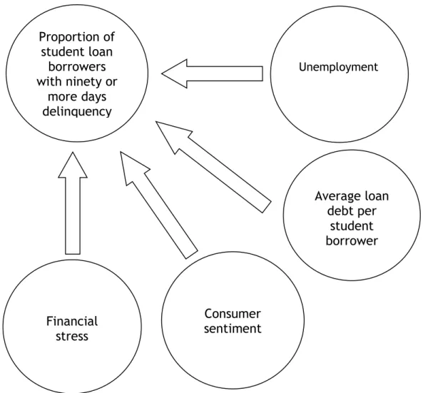
Figure 5 represents a possible response of the proportion of student borrowers with the different independent variables.
20
Figure 5: Representation of a possible response of the proportionof student borrowers with the different independent variables
In this figure, all the independent variables have positive impact in the proportion, meaning that all of them are responsible for higher delinquency or default.
Proportion of
student loan
borrowers
with ninety or
more days
delinquency
or in default
Unemployment
Average loan
debt per
student
borrower
Consumer
sentiment
Financial
stress
21
6. Empirical results
Table 8 reports the random effects linear model and the fractional probit model estimates of the proportion of borrower in ninety or more days delinquency or in default with robust standard errors for the presence of heteroskedasticity.
Table 8: Estimated results with robust standard errors
Dependent Variable is def Linear with random effects model Fractional probit model
Estimate
(Standard error) Estimate (Standard
error) Margin ln(unem) .0125* .0805** .0120 (.0068) (.0405) ln(adb) .0961*** .6524*** .0973 (.0056) (.0324) ln(cs) .0463*** .2735*** .0408 (.0041) (.0276) ln(fstress) .0009 .0092 .0014 (.0012) (.0071) Constant -1.0317*** -8.7882*** (.0587) (.3259) #Observations 450 450 #States 50 50
𝑅
2 .30 Wald𝜒
2 384.06 627.8Note: Dependent Variable is defined in the first row of the Table. Values in parentheses below coefficients are the robust standard errors. Level of significance: *** for p-value >0.01, ** for > 0.05, * for >0.1. The Stata commands xtreg, re vce(robust) and xtgee, family(bionomial) link(probit) corr(exchangeable)
vce(robust) were used.
The linear model has a 𝑅2 of 0.30, which indicates that 30 percent of the variation in
the independent variables is explained in the empirical model. The coefficient of the natural log of unemployment is statistically significant at the 10 percent level, a one percent increase in the natural log of unemployment would lead to an increase of 0.0125 percentage point in the proportion of student borrowers in ninety or more days of delinquency or default. The natural log of the average student debt per borrower is significant at the 1 percent level, and a 1 percent increase in the natural log of the average debt per borrower would lead to a raise of 0.0961 percentage point in the dependent variable. A one percentage point increase in the natural log of the consumer sentiment is associated with a 0.0463 percentage point raise in the dependent variable, and the coefficient is significant at the 1 percent level. The natural log of
22
financial stress has a coefficient of 0.0009 but it is not statistically significant at the 10 percent level.
Since our dependent variable, the proportion of student borrowers in ninety or more days delinquency or in default, is bounded between zero and one, linear models may not provide a rigorous perception for the impacts of some independent variables on the dependent variable throughout the entire distribution. So, for that issue we use the fractional probit model.
In this model, the natural log of unemployment remains positive and statistically significant but at a 5 percent level. The natural log of the average student debt per borrower and the natural log of consumer sentiment also remain positive and statistically significant at the 1 percent level and the natural log of financial stress is still not statistically significant at the 10 percent level. A comparison of the linear model estimates and the fractional probit marginal effects indicates that their order of magnitude is very much alike and the difference in parameter estimates are relatively sizable.
Table 9 reports the random effects linear model and the fractional probit estimates of the proportion of borrower in ninety or more days delinquency or in default with bootstrapped standard errors, with 500 replications used for the presence of heteroskedasticity. Bootstrapping is a nonparametric approach used for the precise estimation of coefficients, standard errors and confidence intervals revealing robust p-values (Guan,2003; Mooney and Duval, 1993).
23 Table 9: Estimated results with bootstrapped standard errors
Dependent Variable is def Linear with random effects
model Fractional probit model
Estimate Estimate Margin
(Standard Error) (Standard Error)
ln(unem) .0125* .0805* .0120 (.0072) (.0423) ln(adb) .0962*** .6524*** .0973 (.0057) (.0343) ln(cs) .0463*** .2735*** .0408 (.0042) (.0269) ln(fstress) .0009 .0092 .0014 (.0012) (.0076) Constant -1.0317*** -8.7881*** (.0587) (.3323) #Observations 450 450 #States 50 50
𝑅
2 .30 Wald𝜒
2 380.82 588.66Note: Dependent Variable is defined in the first row of the Table. Values in parentheses below coefficients are the bootstrapped standard errors. Level of significance: *** for p-value >0.01, ** for > 0.05, * for >0.1. The number of replications used was 500. A random seed was set for each regression. The Stata commands
xtreg, re vce(bootstrap) and xtgee, family(bionomial) link(probit) corr(exchangeable) vce(bootstrap)
were used.
Using the same models with bootstrapped standard errors we obtain the same coefficients and margins but different standard errors from the models with robust standard errors.
In the linear model, the natural log of unemployment is positive and statistically significant at the 10 percent level, the natural log of the average student debt per borrower and the natural log of consumer sentiment are statistically significant at 1 percent level. And the natural log of financial stress remains not statistically significant at the 10 percent level.
In the fractional probit model, the natural log of unemployment is only positive and statistically significant at the 10 percent level. The natural log of the average student debt and the natural log of consumer sentiment are still statistically significant at the 1 percent level and the natural log of financial stress is still not statistically at any level.
So, this sets, linear and fractional probit models, are coherent with prior studies and show us that unemployment (Looney and Yanellis, 2015; Woo, 2002) and the average debt per borrower (Lochner and Monge-Maranjo, 2015; Choy and Li, 2006; Dynarski, 1994) have a positive and statistically significant effect on the proportion of student borrowers on ninety days or more delinquency or in default, implicating when unemployment and average debt increases so does the number delinquencies or default.
25
7. Discussion
Our empirical study on the fractional response of the proportion of student borrowers with ninety days or more delinquency or in default generates the following results. First, there is a significant and positive relationship between unemployment, the average debt per borrower and consumer sentiment with the proportion of delinquent or in default student borrowers. Second, the estimated coefficients on the financial stress variable are not statistically significant. Third, we can see a difference in the estimated coefficients between the fractional probit model and the linear model. Fourth, this is the first attempt to use the fractional probit for a panel data on a student loan delinquency or default data analysis.
The positive relationship between unemployment and the proportion of delinquent or in default student borrowers suggests that, in these period, higher unemployment leads to a higher proportion of delinquent or in default borrowers, which is according to previous literature (Looney and Yanellis, 2015; Woo, 2002). This may occur more often among borrowers with degrees that have high unemployment rates, borrowers with high debt burden that just got unemployed without a considerable amount of savings to repay monthly their loans, and, according to Deming et al. (2012), borrowers from for-profit institutions, who have higher unemployment rates than other types of institutions.
The private and public lenders should be requiring, when lending these loans, higher interest payments to students who choose degrees with high unemployment rates, from for-profit institutions and students that borrow higher amount of loans, when compared to students who choose lower unemployment degrees, from public or non-profit institutions and low amounts of debt, since these represent less risk of default when borrowing a loan.
The positive response of the average debt per borrower and the proportion of delinquency or default indicates that, between these years, students incurring in higher debt have guide to more delinquency or default. This increase in the average debt burden is possibly driven by the raise in the cost of university tuition over the years (Haughwout et al., 2015).
The type of institution might also affect the average debt per borrower (Looney and Yanellis, 2015), but whatever the nature the nature of the institutions, higher debt means higher odds of default (Choy and Li, 2006; Lochner and Monge-Maranjo, 2004; Dynarski, 1994). Student borrowers with low income careers have more problems with unmanageable loan debt than student borrowers who have higher income careers, which have higher chances of repaying their debt (Choy and Li, 2006). The choice for degrees with higher income is also
26
key factor for some student borrowers who incur in high levels of student debt, being the exception in students with high debt level (Woo, 2002; Volkwein et al., 1992).
By other words, degrees that typically have higher wages, cost less to the borrower than degrees that lead to low wage income. Since low income borrowers have a higher risk of default than higher income borrowers, the solution for this problem could also be higher interest payments to cover the risk of default by the low-income borrowers, and also be applied to students from for profit institutes, who have higher level of debt average when compared to other type of institution, representing a bigger risk of default.
In this study, we also find a positive relationship between consumer sentiment and the proportion of student borrowers on delinquency or in default proposing that, in this period, when the consumer is feeling positive about his or her financial health on the short term and economy’s growth in long term causes the raise of the proportion of student borrowers in delinquency or default. The possible cause for this can be, in certain periods, when the consumer is feeling confident with the positive trend of the economy and with his or her financial situation, the consumer might start to think investing in education for better job opportunities and will probably use loans to pay their study costs. This might lead to more defaults, in case the chosen degrees have a high unemployment rate, or low income in a future job, making it unable financially for the borrower to continue the repayments to the lenders.
Other ways to decrease the proportion of delinquency or default can be using the endowment income received by universities from former students, to provide the new qualified students who, otherwise, are unable to possess the financial resources without having to take a loan and having an unmanageable debt.
There can also be a reduction in the number of vacancies or even finishing the existence of some degrees in case these have high unemployment rates and the labor market cannot absorb all these students, and degrees that give only access to low income careers, being higher the risk of not making the repayments on time.
The government can also adopt a higher education system identical to some countries in Europe, which consists in government partially paying the cost of tuitions and the rest is paid by the student. Or, like some other European countries, students don’t have to pay the cost of their education. This could probably lower the proportion of student borrowers in delinquency or default, but it would also mean an increase in the fiscal burden for the taxpayer
.
27
8. Conclusion
In this paper we investigate the response of the proportion of student borrowers with ninety or more days of delinquency or in default to variables such as unemployment and the average debt per borrower, in the United States, using a panel data of 50 states, from 2004 to 2012.
This study is the first experiment to use a fractional probit model for panel data for student borrower delinquency or default data analysis. The existing studies about the US student debt default use data from a specific university or region, in this study we use data of the 50 states.
The empirical evidence has found that unemployment, the average debt per borrower and consumer sentiment are significant in the contribution of ninety days or more delinquency or default, and financial stress is not statistically significant is this study.
Since, this paper shows that unemployment and average debt per borrower have a positive impact and represent a significant risk on delinquency or default, lenders must consider giving higher interest payments to borrowers who will have a higher risk of default, or universities could also limit the number vacancies to degrees with high unemployment rates. Other alternative is the government change its higher education system to one similar with some European countries, which tuitions are partially or fully paid by the state. This could have a significant effect on proportion of student borrowers on delinquency or default.
This study has a limitation of excluding data of the cost of attendance in different type of institutions and the number of student borrowers by state. This could be an area to examine in posterior studies. Future studies should also include countries like England and Australia to compare with the situation in the USA.
29
References
Avery, C., and Turner, S. (2012). Student loans: Do college students borrow too much—or not enough?. The Journal of Economic Perspectives, 26(1), 165-192.
Baum, S., and O'Malley, M. (2003). College on credit: How borrowers perceive their education debt. Journal of Student Financial Aid, 33(3), 1.
Breusch, T. S., and Pagan, A. R. (1979). A simple test for heteroscedasticity and random coefficient variation. Econometrica: Journal of the Econometric Society, 1287-1294. Breusch, T. S., and Pagan, A. R. (1980). The Lagrange multiplier test and its applications to
model specification in econometrics. The Review of Economic Studies, 47(1), 239-253. Cellini, S.R., and R. Darolia. (2015). "College costs and financial constraints: Student borrowing at for-profit institutions." In Student Loans and the Dynamics of Debt, Brad Hershbein and Kevin M. Hollenbeck, eds. Kalamazoo, MI: W.E. Upjohn Institute for Employment Research, 137-174.
Chakrabarti, R., Haughwout, A., Lee, D., Scally, J., and van der Klaauw, W. (2017). Press Briefing on Household Debt, with Focus on Student Debt. Federal Reserve Bank of New
York.
Chamberlain, G. (1982). Multivariate regression models for panel data. Journal of
econometrics, 18(1), 5-46.
Chamberlain, G. (1984). Panel data. Handbook of econometrics, 2, 1247-1318.
Choy, S. P., and Li, X. (2006). Dealing with debt: 1992-93 bachelor's degree recipients 10 years
later. US Department of Education, National Center for Education Statistics, Institute
of Education Sciences.
Christman, D. E. (2000). Multiple realities: Characteristics of loan defaulters at a two-year public institution. Community college review, 27(4), 16-32.
Deming, D. J., Goldin, C., and Katz, L. F. (2012). The for-profit postsecondary school sector: Nimble critters or agile predators?. Journal of Economic Perspectives, 26(1), 139-64. Doornik, J. A., and Hansen, H. (2008). An omnibus test for univariate and multivariate
normality. Oxford Bulletin of Economics and Statistics, 70(s1), 927-939.
Dynarski, M. (1994). Who defaults on student loans? Findings from the national postsecondary student aid study. Economics of Education Review, 13(1), 55-68.
30
Elliott, W., and Nam, I. (2013). Is student debt jeopardizing the short-term financial health of US households?. Federal Reserve Bank of St. Louis Review, 95(September/October 2013).
Federal Reserve Bank of St. Louis, St. Louis Fed Financial Stress Index [STLFSI], retrieved from FRED, Federal Reserve Bank of St. Louis; https://fred.stlouisfed.org/series/STLFSI, February 3, 2018.
Flint, T. A. (1997). Predicting student loan defaults. The Journal of Higher Education, 68(3), 322-354.
FRBNY Consumer Credit Panel / Equifax
Goodell, J. W. (2016). Do for-profit universities induce bad student loans?. The Quarterly
Review of Economics and Finance, 61, 173-184.
Greene, W. H. (2002). LIMDEP: Version 8.0: Econometric Modeling Guide. Econometric Software.
Guan, W. (2003). From the help desk: bootstrapped standard errors. The Stata Journal, 3(1), 71-80.
Han, B. S., Kang, H. G., and Jun, S. G. (2015). Student loan and credit risk in Korea. Economics
Letters, 135, 121-125.
Hardin, J. W., and J. M. Hilbe. (2013). Generalized Estimating Equations. 2nd ed. Boca Raton, FL: Chapman and Hall/CRC.
Harrast, S. A. (2004). Undergraduate Borrowing: A Study of Debtor Students and Their Ability to Retire Undergraduate Loans. Journal of Student Financial Aid, 34(1), 21-37.
Haughwout, A., Lee, D., Scally, J., and van der Klaauw, W. (2015). Student loan borrowing and repayment trends. Report, Federal Reserve Bank of New York.
Herr, E., and Burt, L. (2005). Predicting student loan default for the University of Texas at Austin. Journal of Student Financial Aid, 35(2), 2.
Ionescu, F. (2009). The federal student loan program: Quantitative implications for college enrollment and default rates. Review of Economic Dynamics, 12(1), 205-231.
Ionescu, F., and Simpson, N. (2016). Default risk and private student loans: Implications for higher education policies. Journal of Economic Dynamics and Control, 64, 119-147. Jeffrey, M. W. (2013). INTRODUCTORY ECONOMETRICS: A MODERN APPROACH. CENGAGE
LEARNING.
Knapp, L. G., & Seaks, T. G. (1992). An analysis of the probability of default on federally guranteed student loans. The review of economics and statistics, 404-411.
31
Krishnan, K., & Wang, P. (2018). The Cost of Financing Education: Can Student Debt Hinder Entrepreneurship?. Management Science.
Liang, K. Y., and Zeger, S. L. (1986). Longitudinal data analysis using generalized linear models. Biometrika, 73(1), 13-22.
Lochner, L., and Monge-Naranjo, A. (2004). Education and default incentives with government student loan programs. NBER working paper, 8815.
Looney, A., & Yannelis, C. (2018). Borrowers with Large Balances: Rising Student Debt and Falling Repayment Rates.
Looney, A., and Yannelis, C. (2015). A crisis in student loans?: How changes in the characteristics of borrowers and in the institutions they attended contributed to rising loan defaults. Brookings Papers on Economic Activity, 2015(2), 1-89.
Monge-Naranjo, A. (2014). Recent trends in student loans: more loans and higher balances. Federal Reserve Bank of St. Louis Economic Synopses, 2, 014.
Mooney, C. Z., Duval, R. D., and Duvall, R. (1993). Bootstrapping: A nonparametric approach
to statistical inference (No. 94-95). Sage.
Mundlak, Y. (1978). On the pooling of time series and cross section data. Econometrica: journal
of the Econometric Society, 69-85.
Papke, L. E., and Wooldridge, J. M. (2008). Panel data methods for fractional response variables with an application to test pass rates. Journal of Econometrics, 145(1-2), 121-133 Pesaran, M. H. (2004). General diagnostic tests for cross section dependence in panels. Pesaran, M. H. (2006). Estimation and inference in large heterogeneous panels with a
multifactor error structure. Econometrica, 74(4), 967-1012.
Pinto, M. B., and Mansfield, P. M. (2006). Financially at-risk college students: An exploratory investigation of student loan debt and prioritization of debt repayment. Journal of
student financial aid, 36(2), 2.
Podgursky, M., Ehlert, M., Monroe, R., Watson, D., and Wittstruck, J. (2002). Student loan defaults and enrollment persistence. Journal of Student Financial Aid, 32(3), 27-42. Ramsey, J. B. (1969). Tests for specification errors in classical linear least-squares regression
analysis. Journal of the Royal Statistical Society. Series B (Methodological), 350-371. Rothstein, J., and Rouse, C. E. (2011). Constrained after college: Student loans and early-career
occupational choices. Journal of Public Economics, 95(1), 149-163.
Sánchez, J. M., and Zhu, L. (2015). Student Loan Delinquency: A Big Problem Getting Worse?. Economic Synopses, 2015.