Rui Filipe de Jesus Cabeça

(1)

Rui Filipe de Jesus Cabeça

Licenciatura em Engenharia dos Materiais

Magnetic tweezers for captive disclination loops

Dissertação para obtenção do Grau de Mestre em

Engenharia dos Materiais

Orientadora:

Professora Doutora Maria Helena Godinho, Professora

Auxiliar com agregação,

Faculdade de Ciências e Tecnologia da Universidade

Nova de Lisboa

Júri

Presidente: Prof.Doutor João Paulo Borges Arguente: Prof.João Luis Maia Figueirinhas

(2)

(3)

Magnetic tweezers for captive disclination loops

Copyright cRui Filipe de Jesus Cabeça, 2017.

(4)

(5)

Acknowledgements

Agradeço profundamente à professora Helena Godinho, não só por ter sido a pessoa que me guiou durante todas as etapas deste projecto, mas também por todo o tempo e ajuda que me deu para conseguir ﬁnalizar esta dissertação. O compromisso demonstrado pela mesma foi inalcansável. De salientar também o enorme gosto e motivação com que encarou este projecto.

A very special thank you to Professor Pawel Pieranski, who gave me a lot of guidance and help during my stay in France. I’m grateful for all the help given to carrying out the research work, and for all the morning sessions of learning at the cafeteria.

Um agradecimento especial também ao Professor João Canejo, por toda a ajuda prestada no laboratório, e pelo tempo que dispensou para me ajudar. Devo salientar também a simpatia e alegria com que encara o dia-a-dia.

Uma palavra de apreço para a Ana Almeida, também pelo tempo que dispensou para me ajudar nas tarefas de laboratório, e por ter dispensado as folhas das plantas que utilizei neste projecto.

Quero agradecer ao Professor João Paulo Borges, principalmente pela disponibilidade e ajuda constante que me proporcionou durante todo o curso.

(6)

(7)

Abstract

It is known that Liquid crystals (LCs) are very sensitive to external ﬁelds, making them very desirable regarding technological applications. The uniaxial nematic phase, with long-range orienta-tional order, is widely studied, presenting molecular alignment singularities known as disinclination lines. The manipulation of these lines opens new perspectives in the LCs ﬁeld.

In fact recent studies showed that what appeared to be a point defect in a nematic liquid crystal, are actually nanometer-sized closed-loops[1], that can selectively trigger self-assemble molecular processes.[2]. The disclination loops appearance as well as position, when threaded on polymeric ﬁbers with axial anchoring, can be precisely controlled.

In this work, we present results concerning the generation and precise manipulation these disclination loops, on a micro-scale, threaded on nylon, micro plants cellulose-based filaments and electrospun fibers, immersed in homeotropic nematic cells, with the application of a magnetic field.

(8)

(9)

Resumo

É sabido que os Cristais líquidos são muito sensíveis à aplicação de campos externos, tornando-os assim muito desejáveis no que toca a aplicações tecnológicas. A fase nemática uniaxial, com ordem orientacional de longo alcance, está amplamente estudada, apresentando defeitos no alinhamento molecular denominados linhas de disclinação. A manipulação destas linhas abre novas perspectivas no que toca ao ramo dos cristais líquidos.

Estudos recentes mostram que o que aparenta ser um defeito pontual num cristais líquido nemático, são na realidade anéis de disclinação, à escala nanométrica[1], e estes podem desencadear processos de ordenamento molecular de forma bastante selectiva[2]. O aparecimento destas linhas de disclinação, bem como a sua posição, quando estão enroladas à volta de ﬁbras poliméricas com ancoragem planar, são condições que podem ser facilmente controladas.

Neste trabalho, apresentamos resultados tendo em conta a geração e manipulação precisas destes anéis, à escala micrométrica, quando enrolados em fibras de nylon, em micro filamentos de plantas à base de celulose e fibras de electrospinning, quando inseridas em células nemáticas com ancoragem homeotrópica, recorrendo à aplicação de campos magnéticos.

(10)

(11)

Abbreviations

LC(s) Liquid Crystals

POM Polarized optical microscope HPC Hydroxypropylcellulose 5CB 4’-n-pentyl-4-cyanobiphenyl

EN18 Nematic liquid crystal mixture (∆ξ<0) CCD Charge-coupled device

CA Cellulose acetate

DMac Dimethyllacetamide

(12)

(13)

Symbols

B Magnetic ﬁeld

Cg Chirogyral coeﬃcient

d Sample thickness

∆χ Diamagnetic anisotropy

f Resulting force per unit length

F Elastic energy per unit surface fd Frank’s free energy

fl Laplace force

fr Laplace opposite force

h Distance between the ﬁber and the disclination

K Frank elastic constant

K11 Splay elastic constant

K22 Twist elastic constan

K33 Bend elastic constant

M Magnetization

m Topological charge

m Molecule’s magnetization

Mn Average number molecular weight

ΓM Magnetic torque

n Director

R Fiber’s radius

S Order parameter

T Temperature

Te Disclination line tension

t Time

τ Time constant

ξ(B) Magnetic coherence length

(14)

(15)

Contents

Abbreviations xi

Symbols xiii

List of Figures xvi

1 Introduction 1

1.1 Aims of the present work . . . 1

1.2 Liquid Crystals: Nematic Phase. . . 1

1.2.1 Frank’s continuous elastic theory . . . 2

1.2.2 Surface Anchoring . . . 3

1.2.3 Topological Defects. . . 3

1.2.4 Captive disclination loops on ﬁbers . . . 5

1.2.5 External Fields . . . 5

2 Experimental and Characterization Techniques 7 3 Results and Discussion 9 3.1 Planar Axial Anchoring . . . 9

3.2 Tilted magnetic ﬁeld, translation of disclination loops . . . 10

3.3 Trap-like action of an inhomogeneous magnetic ﬁeld . . . 12

3.4 Captive disclination loops, the chirogyral eﬀect . . . 13

3.5 Generation of captive disclination loops by electrohydrodynamic turbulence . . . . 14

3.6 Magnetic Traps . . . 16

3.7 Field induced translation of disclination loops . . . 20

3.8 Horizontal magnetic ﬁelds on CA electrospinning ﬁbers. . . 22

3.9 Horizontal magnetic ﬁelds on natural ﬁbers . . . 26

4 Conclusions and Future Perspectives 29

Bibliography 30

(16)

List of Figures

1.1 a) POM picture of the nematic phase, between cross-polarizers; b) Schematic represen-tation of the director~n, showing the average orientation of the calamitic molecules, and θ, the deviation between an arbitrary nematic calamitic molecule and the director~n. . 2 1.2 Schematic representation of the diﬀerent types of elastic deformations in nematic liquid

crystal: a) Splay (K11); b) Twist (K22); c) Bend (K33)[9]. . . 3 1.3 POM pictures of: a) a positive integer point defect, under crossed polarizers; b) same

point defect as in a), between cross-polarizers with a 530nm retardation plate; c) same point defect as in a), between parallel polarizers, rotated anticlockwise. It should be noted that the four brushes also rotate counterclockwise, implying that this is a positive integer point defect; d) a Schlieren texture of a nematic liquid crystal, under crossed polarizers, showing positive and negative integer point defects. Schematic representation of some topological defects: e) negative semi-integer, m = −(1/2); f) positive semi-integer,m= +(1/2); g) negative integer,m=−1; h) positive integer,m= +1. . . 4

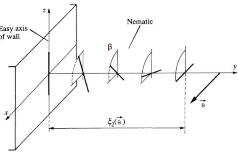
3.1 Schematic representation of a simple twist. The nematic molecules are parallel to thez axis near the wall, and parallel to_B~ _{far from the wall. The applied magnetic field}_B~ _is parallel to thexaxis. As the distance from the wall increases, the nematic molecules present an angleβ, going from0 near the wall, toπ/2far from the wall[8]. . . 10 3.2 Symmetries of the system ”cylinder + field”: a) Planar axial anchoring, no field: D∞h,

for simplicity only one mirror plane parallel to the cylinder axis and one twofold axis orthogonal to it are shown; b) Planar axial anchoring + field orthogonal to the cylinder: D2h; c) Planar axial anchoring + field oblique to the cylinder: C2v; d) Helical anchoring + field orthogonal to the cylinder: D2. . . 11 3.3 Fiber with axial anchoring in the magnetic field orthogonal to it: a) and b) are the two

ground states.. . . 12 3.4 Magnetic ﬁeld of a cylindrical magnet acting as a trap for disclination loops. . . 12 3.5 The chirogyral eﬀect: tilt of the captive disclination loops with respect to the axis of

the ﬁber with a planar helicoidal anchoring inserted in a nematic hoemotropic sample with the director ﬁeld oriented inzdirection. . . 14 3.6 Fiber of diameter D= 28µm, drawn by hand from an anisotropic63%HPC-in-water

(17)

L i s t o f F i g u r e s

3.7 Generation of captive disclination loops by the electrohydrodynamic turbulence: a) one disclination loop captive on a HPC fiber inserted in a homeotropic cell of the nematic EN18; b) stretching of the initial captive disclination loop leads to formation of the strongly light scattering domain DSM2 containing a finite density of disclinations; c) growth of the DSM2 domain; d-g) elastic relaxation after switching the AC field off unveils the existence of six new pairs of disclination loops generated by the turbulent flow. . . 16 3.8 Principle of the experiment. Captive disclination loops threaded on a Nylon fiber,

in-serted into a sample with homeotropic anchoring, ﬁlled with nematic liquid crystal 5CB, are submitted to an oblique and inhomogeneous magnetic ﬁeld created by cylindrical magnets: a) Photograph of setup; b) perspective view of the setup; c) closer view of the setup. . . 17 3.9 Determination of the relaxation timeτ characteristic of the magnetic trap: a) one frame

showing one position of the captive disclination loop around the ﬁber, and the magnet orthogonal to the ﬁber axis; b) reslice of the image sequence. . . 18 3.10 Variation of the shape of the disclination loop, with the increasing of the distance

between the magnets and the ﬁber. The distancedis expressed inµm.. . . 18 3.11 a) Plot of the position of the captive disclination loop versus the time of the movie;

b) Plot of the inverse of time constant versus the inverse of the distance between the disclination loop and the magnets; c) Plot of the time constant versus the distance between the disclination loop and the magnets, represented by the red crosses, and the tilt angle versus the distance between the disclination loop and the magnets, represented by the blue crosses.. . . 19 3.12 Principle of the experiment. Captive disclination loop threaded on a Nylon ﬁber, inserted

into sample with homeotropic anchoring, ﬁlled with nematic liquid crystal 5CB, are submitted to an horizontal homogeneous magnetic ﬁeld, created by two cylindrical magnets: a) Photograph of the setup; b) perspective view. . . 20 3.13 Reslice of the image sequence, showing the increasing of the velocity of the disclination

loop, with the increasing of the ﬁeld angle between the disclination loop and the magnets. 21 3.14 a) Plot of the velocity of the disclination loop versus the ﬁeld angleθ(θ=π−Φ)between

the fiber main axis and the horizontal homogeneous magnetic field created by the two magnets. The plain line in this graph represents the best linear fit to experimental results in the interval[−50◦_,₅₀◦_]_{; b) symmetry relationship explaining the odd dependence of} v onΦ. . . 22 3.15 a) Photograph of the electrospinning setup: 1- infusion pump KDS100; 2- syringe;

3- coaxial shield ring; 4- target. The ﬂow rate, the voltage used and the distance between the needle and the target were, respectively: 0.02mlh−1_,_20kV _and_15cm_{. b)} Photograph of the target, where we can see the plastic frame, coated with double sided adhesive tape, glued on top of the aluminum stripes separated by6mm. . . 23 3.16 Photograph of the setup: 1- magnet; 2- microscope lens; 3- sample; 4- microscope

(18)

L i s t o f F i g u r e s

3.17 POM pictures of cellulose acetate fibers, produced from a CA solution (12%w/w), in a homeotropic sample: a) under crossed polarizers; b) between cross-polarizers with a 530nm retardation plate. The different colors surrounding the fiber, yellow and blue, show us that there are different orientation of the director field~n along the fiber[27]. The average diameter of the fibers is4µm. These fibers induce disclination loops which can be seen easily in these two photographs, that are perpendicular to the fiber main axis, due to the planar anchoring on the fiber surface and the homeotropic anchoring of the sample walls. . . 24 3.18 Picture a captive disclination loop on a nylon fiber, where the equilibrium distanceh,

as well as R, fL and fr are schematically represented. The scale bar corresponds to 50µm. . . 25 3.19 POM pictures of the natural ﬁbers taken from the plant calledOrnithogalum thyrsoides,

(19)

C h a p t e r

1

Introduction

1.1 Aims of the present work

Liquid crystals (LCs) response to electric and magnetic fields enables their widespread tech-nological applications. The uniaxial nematic phase is the most studied and is characterized by a long-range orientational order and the appearance of dark, flexible filaments known as disclinations lines. The precise control of the presence and movement of these lines, corresponding to singulari-ties in the molecular alignment, opens news horizons to LCs applications and to man-made soft materials.

It has been show recently by Xiaoguang Wang et all.[1] that the cores of singular defects appearing optically as point defects are, in fact, nanometer-sized closed-loops. In addition, it was also shown by Xiaoguang Wang et all.[2] that these nanoscopic environments can trigger processes of molecular self-assembly in a very selective way.

In this work, micrometer-sized captive disclination loops will be manipulated by the application of magnetic fields. In particular, the behaviour of these loops, under the action of oblique and/or inhomogeneous magnetic fields, threaded on Nylon, natural and electrospun fibers immersed in homeotropic nematic cells will be addressed. More precisely, in the case of using nylon fibers two different setups will be built: the first one to study the behaviour of the captive disclination loops when submitted to an oblique and inhomogeneous magnetic field created by cylindrical magnets. The trajectory of the disclination loop as function of time, and also the time constant and the tilt angle of the loop, when the distance between the fiber and the magnets is changed, will be calculated; the second setup will allow to study the behaviour of these loops when an horizontal and homogeneous magnetic field, created by two cylindrical magnets is applied, and also the influence on the velocity of the disclination loop when the angle θ between the fiber main axis and the cylindrical magnets is changed.

When using electrospun and natural fibers, horizontal and homogeneous magnetic field will be applied, with the aim to determine the behaviour of the captive disclination loops while using fibers with 1-2µmdiameter, much smaller than the Nylon fiber diameter (∼60µm). Lastly, we will try

to determine the critical diameter from which the disclination loop doesn’t vanish throughout the medium.

1.2 Liquid Crystals: Nematic Phase

(20)

C H A P T E R 1 . I N T RO D U C T I O N

the shape of the container, characteristics from the second one[3]. Liquid crystals, or mesomorphic materials can be classiﬁed in three main groups, based on their structures: nematics, columnar and smetics[4, 5].

Regarding the nematic phase, represented in Figure 1.1 a), which is the most studied among liquid crystalline phases, the anisotropic molecules exhibit long-range orientational order, and no positional order[3, 4], deﬁned by the director~n, schematically represented in Figure 1.1 b)[5, 6, 7].

The deviation between an arbitrary molecule and the director~nis given byθ, schematically shown

in Figure 1.1 b). The fact that not all molecules point in the same direction is due to the existence of thermal ﬂuctuations. The orientational order is expressed by the order parameter[4], given by 1.1[8]:

hSi=1 2h3 cos

2₍_θ₎₋₁_i _(1.1)

Figure 1.1: a) POM picture of the nematic phase, between cross-polarizers; b) Schematic repre-sentation of the director~n, showing the average orientation of the calamitic molecules, andθ, the

deviation between an arbitrary nematic calamitic molecule and the director~n.

The order parameter is a thermodynamic parameter that decreases with increasing temperature, due to the fact that in the isotropic phase the molecules are randomly distributed,S= 0. For an

ideal crystal, the order parameter is equal to 1[6, 7, 9].

Nematics ( from Greek “vηµa” - thread) owes its name to disclination defects, which appeared as threads. These threads have been called "disclination lines" by Frank, and can be easily seen when a nematic phase is observed under polarized light. We will discuss this in more detail along section 1.2.3[4, 6, 10].

1.2.1 Frank’s continuous elastic theory

(21)

inﬂuence of a magnetic ﬁeld:

Fd= 1

2K11(divn)

2₊1

2K22(n·rotn)

2₊1

2K33(n×rotn)

2₋1

2ε0εa(n·B)

2 _(1.2)

Figure 1.2: Schematic representation of the diﬀerent types of elastic deformations in nematic liquid crystal: a) Splay (K11); b) Twist (K22); c) Bend (K33)[9].

Where−1

2ε0εa(n·B)

2_{is the magnetic ﬁeld component. Regarding this equation, the constants}

K11,K22 and K33 are called Frank elastic constants, and refers to the ability of the director to

prevent Splay, Twist and Bend deformations, respectively. These constants are dependent on the nematic temperature, being generally positive, to ensure the stability of the system[6, 7].

1.2.2 Surface Anchoring

Assuming that the Liquid Crystal (LC) is confined between two substrates, which can be subjected to different treatments, the LC’s director can be easily manipulated, depending on the different anchoring conditions of the sample substrates. Several types of molecular orientation can be promoted, where we can distinguish the following two: planar and homeotropic alignment. The first one can be achieved by rubbing the surfaces unidirectionally, which means that the director

nof the nematic liquid crystal stays parallel to the surface, Figure 1.2 a) and b). Regarding the

homeotropic anchoring that is more diﬃcult to achieve than the previous one, due to the fact that most surfaces, including glass, provide planar alignment. In this conﬁguration, the director nis

perpendicular to the surfaces, Figure 1.2 c). To induce this anchoring, usually the substrates are treated with lecithin[13, 15, 16].

1.2.3 Topological Defects

Defects in liquid crystals can be described as specific regions, within the sample, where the orientation of the molecules is ill-defined. They may be caused by a continuous symmetry breaking, when a phase transition occurs, or due to an application of an external field. The existence of these singularities can increase the free energy of the system[7, 17].

Previous studies indicate that defects in LCs can be classiﬁed based on their dimension: point defects, 0-dimensional structure, when the defect is at a point; line defects, or disclination lines, a 1-dimensional structure; and defect walls, a 2-dimensional structure[7, 18]. The topology and the location of these defects, as well as their distributions, may change with temperature, and also with the nematic anchoring conditions[15, 16].

(22)

spots are both point defects, and can have two or four brushes[20]. In the ﬁrst case, these point defects correspond to thin threads, and are associated with the end of singular stable disclinations. These defects are associated with the topological chargem=±(1/2)[21], due to a rotation of the

molecules main axis by±πaround the defect. The topological charge is given by the number of

brushes divided by 4. The positive sign is assigned to clockwise[3]. When there are four brushes, Figure 1.3 a), the topological charge associated is m=±1, due to a rotation of the director by ±2πaround the point[3, 20, 21], corresponding to point defects that are isolated.

Point defects are subdivided in boojums and hedgehogs. The ﬁrst one is a surface point defect, owing to the fact that they can only exist on the boundaries of the medium, and cannot move inside the bulk. On the other side, hedgehogs are called bulk point defects, due to the fact that they can exist either on the surface but also in the volume[10, 18, 20, 21]. They can also also exhibit radial or hyperbolic conﬁguration[17].

Given the equation1.2, we can use the one-constant approximation: K11=K22=K33=K,

and assuming that a disclination line is located in tin the xy plane, the director ﬁeld is given

by: n(r) = [cosθ(x, y), sinθ(x, y),0][22]. Therefore, this gives rise to the equation: fd(r) = 1

2K(θ

2

x+θ2y)[22]. Due to the fact that the system tends to minimize the free energy, we obtain:

▽2

xyθ= 0[3]. Using polar coordinates, and due to the relation betweenθandφ, the equation that describes the director’s conﬁguration around disclinations is given by1.3[3]:

θ(φ) =mφ+θ0 (1.3)

Whereφ= arctan(y/x),θ0 is a constant andmis a positive or negative integer or semi-integer.

Some possible conﬁgurations of~n are schematically represented in Figure 1.3 e)-h)[7].

Figure 1.3: POM pictures of: a) a positive integer point defect, under crossed polarizers; b) same point defect as in a), between cross-polarizers with a 530nm retardation plate; c) same point defect as in a), between parallel polarizers, rotated anticlockwise. It should be noted that the four brushes also rotate counterclockwise, implying that this is a positive integer point defect; d) a Schlieren texture of a nematic liquid crystal, under crossed polarizers, showing positive and negative integer point defects. Schematic representation of some topological defects: e) negative semi-integer,m=−(1/2); f) positive semi-integer,m= +(1/2); g) negative integer,m=−1; h)

(23)

1.2.4 Captive disclination loops on fibers

We have already introduced and discuss the existence of point defects and disclination lines, but regarding the ﬁrst ones, more precisely hedgehogs(m = ±1), they can be transformed into

disclination loops with m = ±(1/2), ﬁrst notice by Lavrentovich and Terentijev[23], when a

transition between radial and hyperbolic hedgehogs occurs[24, 25].

It has been generally admitted that due to their tension disclination loops in nematic liquid crystal inevitably collapse. It has been show recently by M.H. Godinho et all.[26] that this is not the case when disclination loops are threaded on fibers. In particular such captive disclination loops exist in nematic droplets suspended in cellulosic fibers. Later, the behaviour of these loops was studied using hydroxypropylcellulose(HPC) and Nylon fibers, both with planar anchoring, in homeotropic cells containing nematic liquid crystal[27]. In the case of using HPC, or even twisted nylon, the planar anchoring of the nematic becomes helicoidal near the fiber, resulting then, in an effect called Chirogyral Effect, wherein the disclination loop is tilted, instead of being perpendicular to the fiber[27].

1.2.5 External Fields

It is known that nematics are sensitive to external fields, due to the fact that the local orientation of the molecules and the thermal fluctuations of the director can be changed by the application of magnetic or electric fields, leading to changes in the bulk sample[28]. When a magnetic field is applied, the nematic sample tends to be parallel to the field when its diamagnetic anisotropy is positive(∆χ>0), and perpendicular when is negative(∆χ <0)[3, 11]. When a magnetic field(B) is applied, the acquired magnetization by each molecule(m) is given by1.4[4]:

m= 1

µ0

[χ⊥B+ ∆χ(B·n)n] (1.4)

Whereµ0 is the permittivity in free space.

(24)

(25)

C h a p t e r

2

Experimental and Characterization Techniques

Liquid crystal used during the experiments was the nematic liquid crystal 4’-n-pentyl cyanobiphenyl (5CB), exhibiting a nematic phase between 18◦ _{C and 34}◦ _{C, and also the nematic liquid crystal} EN18.

In the ﬁrst setup, the cell containing the nematic liquid crystal was made of two overlapping glass plates with10mmwidth,20mmlength and1mmof thickness. One plate was ﬁxed while the second one, supported by a simple mechanical system, was mobile. More precisely, the distance

hbetween the two plates as well as their parallelism can be controlled. The inner surfaces of the

two glass plates were treated with egg yolk with the aim to induce a homeotropic anchoring of the nematic liquid crystal. The cell was ﬁlled with the nematic liquid crystal 5CB.

The Nylon ﬁber (ﬁshing line0.2mmin diameter) was stretched between the collinear axes of

two stepping motors controlled independently. By this means the fiber can be twisted precisely. The nematic cell, fixed on axyz translation stage, was moved towards the fiber and by this means the Nylon fiber was introduced into the sample.

After this operation, usually one or more captive disclinations loops were formed on the fiber. Otherwise, we had to create a turbulent flow in the sample, by a vigorous motion of the fiber. Such a turbulent flow stretches disclination lines and results in generation of new captive loops. This is going to be explained in more detail in section 3.5. The sample was observed in transmission mode with an optical system made of a microscope objective and a CCD camera.

As shown in Figure 3.8 b), the inhomogeneous magnetic ﬁeld_B~ _{was created by a long cylindrical}

magnet, almost parallel to the z axis. The magnet was supported by a xyz translation stage,

allowing to control its position with respect to the ﬁber and to the disclination loop. We have made a series of experiments in which thezposition of the magnet was kept constant and only the xandy positions were modiﬁed.

When the captive disclination loop is located in the point O (see Figure 3.4) where the ﬁeld

~

B is orthogonal to the ﬁber, it does not move. But if it is located in positions 1 or 1’, where the

magnetic ﬁeld is oblique with respect to the ﬁber, the disclination loop will move in the −xorx

direction, respectively.

(26)

C H A P T E R 2 . E X P E R I M E N TA L A N D C H A R AC T E R I Z AT I O N T E C H N I Q U E S

In the experiment illustrated by the series of eight pictures in Figure 3.6, section 3.5, a ﬁber of diameterD= 28µm, drawn by hand from an anisotropic63%HPC-in-water solution, has been inserted in a homeotropic sample, also treated with egg yolk, of thicknessd= 100µm, through one

of its two free edges. The sample was ﬁlled with the nematic liquid crystal EN18.

In the second setup, as shown in Figure 3.12 a) and b), the liquid crystal cell was assembled from two glass plates separated by a plastic spacer of thickness 0.6mm. The cell was then ﬁxed

with an epoxy glue on the top of a cylindrical support conceived specially for the purpose of the experiment with horizontal magnetic fields. The plans of this support were drawn with the software SolidWorks, and printed using a 3D printer. In order to enable the application of an horizontal and homogeneous magnetic field, a second part - the magnet holder - was build by the same method. It had a shape of a ring equipped with radial cylindrical holes in which magnets were inserted. The inner diameter of the ring was identical with the outer diameter of the first part, so that magnets can be rotated around thez axis, see Figure 3.12 a). Like in the previous experiment, the Nylon fiber was stretched between the axes of stepping motors, and introduced into the sample, as shown in Figure 3.12 a).

The motion of the captive disclination loop driven by the horizontal and homogeneous magnetic ﬁeld was recorded, and analyzed in the same way as in the previous experiment.

The electrospinning ﬁbers were prepared from cellulose acetate (CA), obtained from12%CA (Mn= 50000gmol−1), in a homogeneous mixture of66.6%(w/w) acetone and33.3%(w/w) DMac. The viscous solution was poured into a2mlsyringe with4.5mmdiameter ﬁtted with a 27-gauge

needle, with0.2mlinner diameter. The syringe was then placed on a infusion pump (KDS100), to

control the ﬂow. The conducting ring with 15 cm in diameter was held coaxially with the needle tip, and electrically connected to it. Then they were both connected with a positive output of a high voltage supply (Glassman EL 30kV). After applying the electric potential, the highly viscous CA solution was fed to the syringe-tip as a constant ﬂow rate of0.02mlh−1_{. The voltage used was}

20kV, and the distance between the nozzle and the collector was 15cm. The setup is illustrated in Figure 3.15 a). The ﬁber collectors was made of a plastic frame (6×22mm), coated with double

sided adhesive tape, glued on top of two aluminum stripes distanced 0.6cmfrom each other, see

Figure 3.15 b). During the process the humidity was around 50%at room temperature, 24◦ C. The samples were made of two overlapping glass plates (10mm × 20mm2_),₁_mm_{of thickness,}

threated with lecithin as well, and the plastic support containing the suspended ﬁbers was placed in the middle. An epoxy glue was used to seal the sample. The samples were then ﬁlled with nematic 5CB.

The natural ﬁbers used in the experiments were taken from the plant called Ornithogalum thyrsoides[29], and they were suspended in the same plastic support. The samples were prepared

(27)

C h a p t e r

3

Results and Discussion

3.1 Planar Axial Anchoring

Let us consider ﬁrst a cylinder with planar axial anchoring~a//~x (see Figure 3.2) , immersed in

a nematic. In the absence of ﬁelds and other surface conditions the director ﬁeld~nwould take the

direction parallel to the cylinder axis~x. The symmetry of this ground state is D∞h (see Figure 3.2 a)).

When a magnetic field_B~ _{is applied in the direction}_~z_{orthogonal to the cylinder, the symmetry} D∞h is broken into D2h (see Figure 3.2 b)) and the director field will be distorted: far from the cylinder it will take the direction of the field while on the cylinder surface it will remain parallel to

~x.

As shown in Figure 3.3 two distorted ground states a) and b) are possible. Taken separately they are symmetrical only with respect to the longitudinal mirror planexz and to the twofold axis

C2//~yorthogonal the ﬁeld. All other symmetry operations of the groupD2h(mirror planesxyand

yz and the two-fold axisC2// ~B) exchange the two ground states.

The same symmetry breaking occurs when the cylinder immersed in a nematic is submitted to the action of glass plates with homeotropic anchoring[30].

In the two ground states generated by the magnetic ﬁeld, the distorsion is localized in a cylindrical shell whose thickness is given by the so-called magnetic coherence length ξ[8], which

due to its importance must be explained in more detail, starting with the case of a simple twist. First, we have to take into account the effects of a magnetic field and a wall on the alignment of the nematic molecules, in the case where the wall is in the xoyplane, and the magnetic fieldB~ is

applied in parallel to the xaxis, as shown in Figure 3.1. We can observe that near the wall the

nematic molecules are parallel to thez axis, and far from the wall they are parallel toB~[8]. This

means that there is a transition layer, near the wall, where the molecules are parallel to it, with the addition of presenting an angleβ(y)with the z direction, as represented in Figure 3.1. This

can be classiﬁed as a distorted state, where the magnetic torque ΓM acting on the magnetization M is given by3.1[8]:

ΓM=χa(n·B)n×B (3.1)

Taking that into account, in this case,ΓMis parallel to theyaxis, and considering a section(1×1cm)

in the xoyplane, from y to y+dy, the section experiences a surface and a bulk torque. Adding

these torques, the equilibrium equation is given by 3.2:

K2d 2_β

dy2 +χaB

(28)

C H A P T E R 3 . R E S U LT S A N D D I S C U S S I O N

Figure 3.1: Schematic representation of a simple twist. The nematic molecules are parallel to the

z axis near the wall, and parallel toB~ far from the wall. The applied magnetic ﬁeldB~ is parallel

to the xaxis. As the distance from the wall increases, the nematic molecules present an angle β, going from 0near the wall, toπ/2 far from the wall[8].

Whereξ2(B~)is a length deﬁned by3.3:

ξ2(B) = (K2χa)1/2/B (3.3)

Substituting in the equation3.2and integrating, and due to the fact that far from the wallβ =π/2,

we come to the equation3.4:

ξ2

dβ

dy =±cosβ (3.4)

Where both solutions are possible. Choosing one of them, and resolving the equation by using a change of variable[8], the result is given by3.5:

t=exp(−y/ξ2) (3.5)

Wheret= tan(π/2)₂−β. This shows thatξ2(B)can be considered as the transition layer.

Regarding a diﬀerent case, where the applied magnetic ﬁeld_B~ _{is parallel to the}_y _{axis, it is not}

just a case of a simple twist, but a combination of splay and bend[8]. These distortions are associated with the elastic constants K11and K33, respectively, where their lengths (ξi) are similar. Thus, using the one-constant approximation already discussed in section 1.2.3 (K11=K22=K33=K),

the magnetic coherence length is given by 3.6[8]:

ξ(B) =

s µ0K

χa 1

B (3.6)

and the elastic energy per unit surface of the distorted boundary layer is given by:

F =1 2

K

ξ (3.7)

3.2 Tilted magnetic field, translation of disclination loops

When the magnetic ﬁeld is oblique to the cylinder (for example tilted in the direction of thex

(29)

Figure 3.2: Symmetries of the system ”cylinder + field”: a) Planar axial anchoring, no field: D∞h, for simplicity only one mirror plane parallel to the cylinder axis and one twofold axis orthogonal to it are shown; b) Planar axial anchoring + field orthogonal to the cylinder: D2h; c) Planar axial anchoring + field oblique to the cylinder: C2v; d) Helical anchoring + field orthogonal to the cylinder: D2.

no more related by any symmetry operation. If the angle between the magnetic ﬁeld and cylinder is writen as:

π

2 −Φ =

π

2(1−ǫ) (3.8)

whereǫ <<1, then the distortion energy of statesa andbbecomes:

Fa/b = (1±ǫ)2

K

2ξ (3.9)

When the two possible statesaand b coexist on the ﬁber, there must be a disclination loop at the

junction between them. This can be easily checked by following the director orientation on the circuit 12341 drawn with dashed line in Figure 3.3. At the starting point 1 the director is (0,0,1) while after the whole turn of the circuit it becomes (0,0,-1).

The energies per unit surface of the boundary layers adjacent to the disclination loopFa and

Fb can be seen as forces per unit length pulling on the loop, respectively, in−~xand~xdirections. The resultant force

f =Fb−Fa =−2K

ξ

2

πΦ (3.10)

will pull the loop in the~xdirection when the tilt angle of the magnetic ﬁeld~Φis positive. As a result, the disclination loop will move in the~xdirection, as observed in experiments.

When other disclination loops coexist on the ﬁber then their sequence can represented as:

a−DL1−b−DL2−a−DL3−b... (3.11)

In this sequence, the ground statesaandbare located respectively on left and right sides of loops

DL1 andDL3. In the case of the loopDL2 the positions of the ground states are inverted so that

(30)

Figure 3.3: Fiber with axial anchoring in the magnetic ﬁeld orthogonal to it: a) and b) are the two ground states.

3.3 Trap-like action of an inhomogeneous magnetic field

Knowing that the magnetic field oblique with respect to the fiber generates the forcef propor-tional to the field angleΦ (see equations3.8 and 3.10) we are prepared to analyse the action of inhomogeneous magnetic fields such as the one of the cylindrical magnet used in our experiments.

As shown in Figure 3.4, the magnetic ﬁeld of a cylindrical magnet has the axial symmetry with respect to the magnet axis~z.

Figure 3.4: Magnetic ﬁeld of a cylindrical magnet acting as a trap for disclination loops.

In this geometry, the angleΦbetween the field and the axisy normal to the fiber varies as a function of the position xof the loop. In the first approximation, we can write:

(31)

Then, using the equations3.8and3.10we obtain:

f =−Bx (3.13)

with

B= 2K

ξ

2

π (3.14)

Upon the action of the force f the dislocation loop with move with the velocity v given by:

B=v= dx

dt =µf (3.15)

whereµis the mobility.

Finally using equation3.13and3.15we obtain the equation of motion:

dx

dt =−µBx (3.16)

Its solution:

x(t) =x0e−t/τ (3.17)

3.4 Captive disclination loops, the chirogyral effect

As already introduced in section 1.2.4, the ﬁrst observations of captive disclination loops were made in experiments with nematic[31] and cholesteric droplets[26] threaded on HPC ﬁbers with planar anchoring. When the anchoring at the nematic (cholesteric)/air is homeotropic, each droplet must contain, for topological reasons, a defect with the topological charge m= 1: a disclination loop equivalent to a radial hedgehog.

Captive disclination loops were also observed on glass ﬁbers with homeotropic anchoring im-mersed in planar nematic samples[32, 33]. In this geometry, disclination loops were generated in a controlled manner by the KibbleZurek mechanism during quenching from the isotropic into the nematic phase.

Recently, captive disclination loops were created and studied using HPC and Nylon fibers with a planar anchoring immersed in homeotropic nematic samples[27]. In the case when the planar anchoring on the fiber surface was helicoidal, due to the chirality of the polymer (HPC) or to the mechanical torsion of the fiber, the so-called chirogyral effect was observed (see Figure 3.5): the captive disclination loops are tilted with respect to the fiber axis by the angle η which is proportional in the first approximation to the helix angleα:

η=Cg(D/d)α (3.18)

The chirogyral coefficientCg(D/d)occurring in this formula, is a function of the ratioD/dbetween the fiber diameterD and the sample thicknessd. In these first experiments, for symmetry reasons,

disclination loop were rotating around the axis z parallel to the homeotropic anchoring on the sample surfaces.

(32)

Figure 3.5: The chirogyral effect: tilt of the captive disclination loops with respect to the axis of the fiber with a planar helicoidal anchoring inserted in a nematic hoemotropic sample with the director field oriented in zdirection.

3.5 Generation of captive disclination loops by electrohydrodynamic

turbulence

In the experiment illustrated by the series of eight pictures in Figure 3.6, and already intro-duced in section 2, the sample contained, initially, one disclination loop threaded on the ﬁber. Subsequently, we applied a 100Hz, 50V, AC voltage to this EN18 sample with the negative

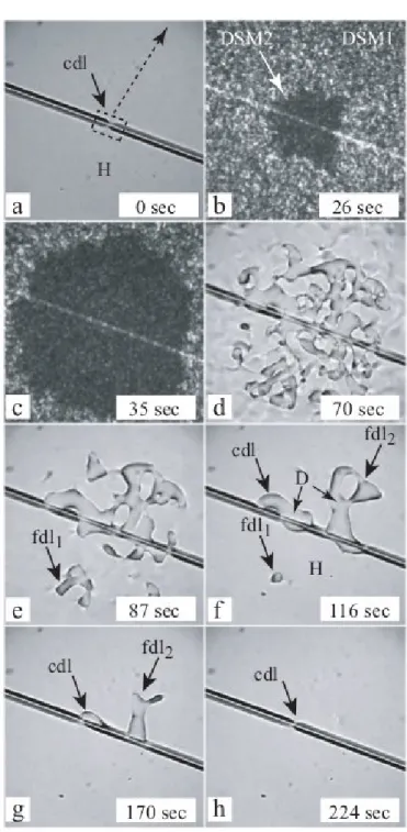
di-electric anisotropy drove the electrohydrodynamic turbulence which stretched progressively the initial disclination loop and created the strongly light scattering area labelled DSM2 whose size is growing with time[35] as shown in Figures 3.6 b) and c). After switching the excitation oﬀ, due to the elastic relaxation, the density of disclination (length/unit volume) is rapidly falling down and a tangle of individual disclination can be distinguished in Figure 3.6 d). In Figure 3.6 f) only three loops are left. Their evolution in Figures 3.6 g) and h) shows that the one labeled cdlis captive

and while the other two, f dl1 andf dl2, are free and can collapse.

(33)

Figure 3.6: Fiber of diameter D= 28µm, drawn by hand from an anisotropic63%HPC-in-water solution, has been inserted in a homeotropic sample, treated with egg yolk, of thicknessd= 100µm,

(34)

Figure 3.7: Generation of captive disclination loops by the electrohydrodynamic turbulence: a) one disclination loop captive on a HPC fiber inserted in a homeotropic cell of the nematic EN18; b) stretching of the initial captive disclination loop leads to formation of the strongly light scattering domain DSM2 containing a finite density of disclinations; c) growth of the DSM2 domain; d-g) elastic relaxation after switching the AC field off unveils the existence of six new pairs of disclination loops generated by the turbulent flow.

3.6 Magnetic Traps

With the purpose of studying the behavior of the captive disclinations loops threaded on nylon ﬁbers, inserted in a sample with homeotropic anchoring, when an oblique and inhomogeneous magnetic ﬁeld _B~ _{is applied, we build a setup, illustrated in Figure 3.8, and already explained in}

the beginning of section 2.

(35)

is now oblique with respect to the ﬁber, and will move in the−x~ direction, toward the positionO,

with a velocityv. The same will happen if the disclination loop is positioned in the1′ _position, and the magnets near the position 1, resulting in the movement of the disclination loop in the~x

direction, toward the position O. In this case, the position of the magnets was only changed in

the~xdirection. For each position of the magnets, a sequence of images was recorded, usually with

a rate of one image every twenty seconds. The positions of the captive disclination loop versus the time of the movies are plotted in Figure 3.11 a). After that, we moved the magnets in the

~xdirection, but also in the−~y direction, increasing the distance dbetween the magnets and the

ﬁber. A sequence of images was recorded in the same way, for increasing distances.

Figure 3.8: Principle of the experiment. Captive disclination loops threaded on a Nylon fiber, inserted into a sample with homeotropic anchoring, filled with nematic liquid crystal 5CB, are submitted to an oblique and inhomogeneous magnetic field created by cylindrical magnets: a) Photograph of setup; b) perspective view of the setup; c) closer view of the setup.

The image sequences recorded were analyzed using the software ImageJ. They were converted to grayscale, and imported as stacks. A typical image from one stack is shown in Figure 3.9 a). The segment AB visible here is parallel to the ﬁber, and crosses the disclination loop. Using the “reslice” command this segment was extracted from each image of the stack and the set of all segments was assembled into the image shown in Figure 3.9 b). Let us note that the segment AB is rotated by 90 degrees with respect to the Figure 3.9 a). It is obvious that the reslice image represents the trajectory x(t) of the loop as a function of time. At the ﬁrst sight, the shape of this trajectory seems to be exponential.

(36)

adjustable parameters coeﬃcientsx0 andτ.

x(t) =x0e−t/τ (3.19)

The inverse of the relaxation time1/τ was then plotted in Figure 3.11 b) as a function of the

inverse of the distancedbetween the magnet and the ﬁber. Let us emphasize that both axes of the

plot in Figure 3.11 b) are logarithmic. The reason for such a choice is that the expected dependence between1/τ and1/dis approximatively given by the power low3.20:

1

τ =a

1

d α

(3.20)

In such a log-log plot the exponent α corresponds to the slope of a straight line ﬁtting the

experimental points. The time constant τ and the tilt angleη versus the distance between the

disclination loop and the magnets are represented in Figure 3.11 c). The shape of the disclination loop with the increasing of the distance between the magnet and the ﬁber is represented in Figure 3.10.

Figure 3.9: Determination of the relaxation timeτcharacteristic of the magnetic trap: a) one frame

showing one position of the captive disclination loop around the ﬁber, and the magnet orthogonal to the ﬁber axis; b) reslice of the image sequence.

(37)

(38)

The Figure 3.11 b) shows clearly that the increasing of the distance between the disclination loop and the magnets translates into a increasing of the time constant. There is also a decreasing of the tilt angle of the disclination loops with the increasing ofd, represented in Figure 3.11 c) and

Figure 3.10.

These results are in agreement with the theoretical analysis in sections 3.1, 3.2 and 3.3.

3.7 Field induced translation of disclination loops

In this section, we studied the behavior of the captive disclination loops threaded on nylon ﬁbers, inserted in a sample with homeotropic anchoring, when subjected to an horizontal and homogeneous magnetic ﬁeld _B~_{, created by two cylindrical magnets. For this purpose, a second}

setup was build, already described in section 2, and illustrated in Figure 3.12.

After inserting the nylon ﬁber into the sample, the magnets were initially placed in the magnet holder with an angle θ = 0, wherein θ = π−Φ. This means that, in the beginning of the

experience,the magnets were parallel to the ﬁber main axis (see Figure 3.12 b)). The angle θ

ranged from0to2π, every 5 degrees, around thezaxis, clockwise, with the help of a circumference

made of paper with lines drawn every 5 degrees. We recorded sequences of images of a loop moving upon the action of an horizontal and homogeneous magnetic ﬁeld for each angle θ.

(39)

The analysis of the image sequences was then identical to what was done in section 3.5. For example, on the spatio-temporal cross section obtained by the reslice command (see Figure 3.13) the velocity of the disclination loop is given by the slope of the trajectory x(t). As we can see

here, there are discontinuous changes of the slope because during this experiment the angle θhas

been changed several times. For a better accuracy the velocity as a function of θ was obtained

from a series of movies recorded at diﬀerent angles θ. The results are plotted in Figure 3.14 a).

Obviously there is a wide range of angles Φ, whereΦ =π−θ, in which velocity is proportional

to Φ. We noticed a linear behavior of v(Φ) in the vicinity ofΦ = 0, due to symmetry reasons represented in Figure 3.14 b). The scheme on the right represents the distortion of the director field in the presence of the magnetic field withΦ>0. When the field is strong enough the distortion

is localized in a cylindrical shell whose thickness is given by the magnetic coherence length ξ(B).

The energy per unit length (in x direction) of this cylindrical shell can be seen as a force pulling on the disclination loop. Clearly, as the distorsion on the left side of the disclination loop (labeled

▽) is larger then on its right side (labeled△), the resulting force drives the motion of the loop to the left as shown. Upon the reversal of the sign of the director field is transformed by reflection in the mirror orthogonal to the fiber and the sign of the loop’s velocityv is reversed too.

Analytically, for this symmetry reason, in the expansion ofv(Φ) into a Fourier series only sine terms sin(mΦ)can occur. Moreover, as the distorsion should not depend on the sign of Bmust

be pair so that ﬁnally one gets the expression:

v(Φ) =asin(2Φ) +bsin(4Φ) +... (3.21)

which in the limit of small anglesΦleads to a linear dependence ofv onΦ:

v=dx

dt ≈αΦ (3.22)

Remarkably, the experimentally observed linear dependence ofv onΦ(see Figure 3.14 a)) is not limited to the vicinity ofΦ = 0but holds in a wide interval of angles−60◦_<_Φ_<₆₀◦_.

The ﬁt of this linear dependence to experimental results in Figure 3.14 a) leads to a positive coeﬃcientα.

(40)

Figure 3.14: a) Plot of the velocity of the disclination loop versus the field angle θ(θ = π−Φ) between the fiber main axis and the horizontal homogeneous magnetic field created by the two magnets. The plain line in this graph represents the best linear fit to experimental results in the interval[−50◦_,₅₀◦_{]; b) symmetry relationship explaining the odd dependence of}_v _on_Φ.

Let us emphasize that these results are in agreement with the theoretical analysis in sections 3.1, 3.2 and 3.3.

3.8 Horizontal magnetic fields on CA electrospinning fibers

As previously mentioned in section 2, the ﬁbers used in this experiment were produced by electrospinning, which due to its importance must be detailed. The process begins whit the placement of the syringe containing a polymeric solution on the pump. In our experiment we used a CA solution. The pump forces the solution to come out at a constant rate of0.02mlh−1_{, and}

due to the application of an high potential to the nozzle (20kV), a drop is formed. The charged

(41)

well as the target, can be observed in Figure 3.15 a) and Figure 3.15 b), respectively.

During the process is necessary to control not only the distance between the needle and the target, but also other critical parameters, such as the humidity and the temperature of the room, as well as the concentration and the viscosity of the polymeric solution[38].

Figure 3.15: a) Photograph of the electrospinning setup: 1- infusion pump KDS100; 2- syringe; 3-coaxial shield ring; 4- target. The ﬂow rate, the voltage used and the distance between the needle and the target were, respectively: 0.02mlh−1_,₂₀_kV _and₁₅_cm_{. b) Photograph of the target, where}

we can see the plastic frame, coated with double sided adhesive tape, glued on top of the aluminum stripes separated by6mm.

As already explained, the samples were prepared by overlapping two glass plates, previously treated with egg yolk, and the support with the suspended fibers was placed in the middle. To study the presence of disclination loops on these fibers, and their behavior when a horizontal and homogeneous magnetic field is applied, we used a different setup from the first two, illustrated in Figure 3.16. For this purpose, a regular polarized light microscope was used. First, without applying the magnetic field, the sample was simply placed in the microscope platinum, to see the presence of the disclination loops, and several pictures were taken with the following microscope lenses: 10x, 20x and 50x. The sample was observed using the transmission mode of the microscope. Some POM pictures are illustrated in Figure 3.17, where we can easily see the presence of these disclination loops.

(42)

the sample was heated by conduction. We used a high heating value due to the energy losses that occur due to the size of the strip.

Figure 3.16: Photograph of the setup: 1- magnet; 2- microscope lens; 3- sample; 4- microscope platinum; 5- magnet holder. Electrospinning fibers inserted in a sample with homeotropic anchoring, and filled with the nematic liquid crystal 5CB, are submitted to an horizontal and homogeneous magnetic field, created by two cylindrical magnets. The angle between the fibers main axis and the magnets is controlled by the angles marked in the platinum. The microscope used is a polarized light microscope.

Figure 3.17: POM pictures of cellulose acetate ﬁbers, produced from a CA solution (12%w/w),

in a homeotropic sample: a) under crossed polarizers; b) between cross-polarizers with a530nm

retardation plate. The different colors surrounding the fiber, yellow and blue, show us that there are different orientation of the director field~nalong the fiber[27]. The average diameter of the fibers

is4µm. These ﬁbers induce disclination loops which can be seen easily in these two photographs,

that are perpendicular to the ﬁber main axis, due to the planar anchoring on the ﬁber surface and the homeotropic anchoring of the sample walls.

After applying the horizontal and homogeneous magnetic ﬁeld to the sample, varying the angle

θ, the image sequences recorded were analyzed using the software VLC media player. Unlike what

(43)

across the ﬁber with a velocityv, in this case the captive disclinations loops remained in the same

place, not showing any movement. This occurred in both phases, and for both values of θ. The cause for such an occurrence could be explained by the fiber diameter. In the case of the nylon fiber, the diameter was200µm(see Figure 3.18). In this case, we have fibers of smaller dimensions,

with approximately4µm, see Figure 3.17. This can indicate that there is a critical diameter from

which the disclination loop does not move, due to the attraction forcefL (see Figure 3.18) that the ﬁber exerts on the disclination loop.

We also noticed that although the disclination loops did not move, the fibers showed slight fluctuations when the field was applied in the liquid crystalline phase and in the isotropic phase. The fact that they have moved in the isotropic phase shows us that the nematic liquid crystal does not interfere with the fiber movement, being only due to the action of the magnetic forces created by the two magnets[39].

In order to know the critical diameter from which the disclination loop doesn’t vanish throughout the medium, it is necessary to do some calculations. It is known that there are two forces acting on a disclination loop, the Laplace force (fL),3.23, andfrwhich is opposed to the ﬁrst one, 3.24, respectively[4]:

fL=

Te

R+h (3.23)

fr= 2πK

m2

2h (3.24)

Wherehis the distance between the ﬁber and the disclination;Ris the ﬁber’s diameter; Kis the

isotropic elasticity;mis the disclinations line strength andTeis the disclinations line tension. The parameters hand R, as well as the two forces fL and fr are schematically represented in Figure 3.18.

Figure 3.18: Picture a captive disclination loop on a nylon ﬁber, where the equilibrium distance h,

(44)

Taking into account that the radius of the ﬁber is much larger thanh(R >> h), comes that:

fL≈

Te

R (3.25)

Due to the fact that the disclination ring is in equilibrium and doesn’t move across the ﬁber, it comes:

fr=fL=

Te

R = 2πK m2

2h (3.26)

Finally, and knowing thatm= +1/2, the ﬁnal expression to the equilibrium distancehis given

by[6]:

h=RπK

4Te

≈RK Te

(3.27)

3.9 Horizontal magnetic fields on natural fibers

After preparing the samples in the same way as the previous ones, they were observed also using a transmission mode microscope. The POM pictures are represented in Figure 3.19. The samples were also submitted to an horizontal and homogeneous magnetic ﬁeld, using the same setup and conditions as already explained in section 3.7.

Figure 3.19: POM pictures of the natural ﬁbers taken from the plant calledOrnithogalum thyrsoides,

in a homeotropic sample: a) under crossed polarizers; b) between cross-polarizers with a530nm

retardation plate; c) between parallel polarizers. We can easily see that these ﬁbers also induce disclination loops. Through a close observation of the picture b), we noticed that the direction of the nematic molecules in the regions near the disclination loops varies. This could be seen by the change of colors between yellow and blue[27]. The average diameter of the ﬁbers is2µm.

In a first analysis, we can say that these disclination loops do not exist only in synthetic fibers, like the previous ones, but also in fibers extracted from natural plants.

After applying the horizontal and homogeneous magnetic ﬁeld to the sample, givingθthe same

(45)

(46)

(47)

C h a p t e r

4

Conclusions and Future Perspectives

While topological defects should be avoided in nematic liquid crystal electro-optical sensors and displays this work demonstrates that 1D defects, i.e. disclination lines, can have some use if precisely designed and manipulated. In particular, it is possible to generate the so-called captive disclination loops threaded on ﬁbers immersed in nematic cells.

It has been pointed out that such captive disclination loops can be manipulated, i.e. translated and tilted, by electric and magnetic ﬁelds.

Tilting captive disclination loops in electric or magnetic fields was found to be a source of information about the fibers morphologies. Indeed, the field-induced tilt of a disclination loop with respect to the fiber axis is correlated with the fibers’ chirality (for fibers with diameters ranging from hundred to few micrometers).

Captive disclination loops have also been put in a translational motion by the action of a magnetic field oblique to fibers and their velocities were found to vary as a function of the field intensity and orientation as well as of the fibers’ diameters. While velocities of 2µm s−1 _were

achieved for rings moving along ﬁbers with diameters of200µm driven by the action of an oblique

magnetic ﬁeld, no motion was observed, using the same drive driving conditions, if ﬁbers with diameters of the order of1−1.5µm were used. A reason for this behavior was given considering

the disclination tension line, which is highly dependent on the radius of the ﬁber: h=RπK

4Te.

(48)

Bibliography

[1] X. Wang, Y.-K. Kim, E. Bukusoglu, B. Zhang, D. S. Miller, and N. L. Abbott. “Experimental Insights into the Nanostructure of the Cores of Topological Defects in Liquid Crystals”. In:

Physical review letters116.14 (2016), p. 147801.

[2] X. Wang, D. S. Miller, E. Bukusoglu, J. J. de Pablo, and N. L. Abbott. “Topological defects in liquid crystals as templates for molecular self-assembly”. In: Nature materials 15.1 (2016),

pp. 106–112.

[3] F. J. Antonio. “Estudo de Defeitos Topológicos em Cristais Líquidos do Ponto de Vista Cosmológico”. Master’s Thesis. Universidade Estadual de Maringá, 2009, p. 121.

[4] P. Pieranski, Pawel, Oswald. Nematic and Cholesteric Liquid Crystals. Taylor & Francis,

2005, p. 616.

[5] M. Cardoso. “Contribuição para o Estudo da Fase Nemática Biaxial em Dendrímeros Líquido-Cristalinos Termotrópicos”. Master’s Thesis. Instituto Superior Técnico, 2007, p. 68. [6] A. de Oliveira. “Cellulose micro/nano ﬁbers conformational eﬀects probed by nematic liquid

crystal droplets”. Master’s Thesis. FCT, 2014, p. 38.

[7] A. Sengupta. Topological microfluidics: nematic liquid crystals and nematic colloids in microfluidic environment. Springer Science & Business Media, 2013.

[8] J. de Gennes and J Prost. The physics of liquid crystals. 83. Oxford University Press, 1995.

[9] S. Čopar. “Topology and geometry of nematic braids”. In: Physics Reports 538.1 (2014),

pp. 1–37.

[10] G. Volovik and O. Lavrentovich. “Topological dynamics of defects: boojums in nematic drops”. In: Zh Eksp Teor Fiz 85.6 (1983), pp. 1997–2010.

[11] D. D. Luders. “Estudo de propriedades ópticas de uma fase nemática calamítica”. PhD Thesis. Universidade Estadual de Maringá, 2014, p. 123.

[12] D. Andrienko. “Introduction to liquid crystals”. In: IMPRS school, Bad Marienberg(2006).

[13] R. A. Alla. “On the Control of Nematic Liquid Crystal Alignment”. PhD Thesis. University of Gothenburg, 2013, p. 49.

[14] F. C. Frank. “I. Liquid crystals. On the theory of liquid crystals”. In: Discussions of the Faraday Society 25 (1958), pp. 19–28.

[15] C. M. Tone, M. P. De Santo, M. G. Buonomenna, G. Golemme, and F. Ciuchi. “Dynamical homeotropic and planar alignments of chromonic liquid crystals”. In: Soft Matter 8.32 (2012),

pp. 8478–8482.

[16] C. Tone, M. De Santo, and F Ciuchi. “Alignment of chromonic liquid crystals: A diﬃcult

(49)

B I B L I O G R A P H Y

[17] T. Lubensky, D. Pettey, N. Currier, and H. Stark. “Topological defects and interactions in nematic emulsions”. In: Physical Review E 57.1 (1998), p. 610.

[18] M. Kleman and O. D. Lavrentovich. “Topological point defects in nematic liquid crystals”. In: Philosophical Magazine 86.25-26 (2006), pp. 4117–4137.

[19] J. Nehring and A. Saupe. “On the schlieren texture in nematic and smectic liquid crystals”. In:

Journal of the Chemical Society, Faraday Transactions 2: Molecular and Chemical Physics

68 (1972), pp. 1–15.

[20] J. de Gennes. “Nematic Liquid Crystals: Defects”. In: I (1993), pp. 1–5.

[21] O. Lavrentovich. “Defects in liquid crystals: surface and interfacial anchoring eﬀects”. In:

Patterns of Symmetry Breaking. Springer, 2003, pp. 161–195.

[22] G. Vertogen and W. H. de Jeu. Thermotropic liquid crystals, fundamentals. Vol. 45. Springer

Science & Business Media, 2012.

[23] O. D. Lavrentovich and E. M. Terentjev. “Phase transition altering the symmetry of topo-logical point defects (hedgehogs) in a nematic liquid crystal”. In: Soviet Physics JETP

64.December 1986 (1986), pp. 1237–1244.

[24] Y.-S. Wang, B.-H. Yuan, and G.-H. Yang. “Eﬀect of Saddle-Splay Elasticity on Stability of Disclination Rings in Nematic Liquid Crystals”. In: Communications in Theoretical Physics

50.4 (2008), pp. 847–850.

[25] G. P. Alexander, B. G. G. Chen, E. A. Matsumoto, and R. D. Kamien. “Colloquium: Disclination loops, point defects, and all that in nematic liquid crystals”. In: Reviews of Modern Physics84.2 (2012), pp. 497–514.

[26] Y Geng, D Seč, P. L. Almeida, O. D. Lavrentovich, S Žumer, and M. H. Godinho. “Liquid crystal necklaces: Cholesteric drops threaded by thin cellulose ﬁbres”. In: Soft Matter 9.33

(2013), pp. 7928–7933.

[27] S. Čopar, D. Seč, L. E. Aguirre, P. L. Almeida, M. Dazza, M. Ravnik, M. H. Godinho, P. Pieranski, and S. Žumer. “Sensing and tuning microﬁber chirality with nematic chirogyral eﬀect”. In: Physical Review E 93.3 (2016), p. 032703.

[28] B. J. Frisken. “Nematic liquid crystals in electric and magnetic ﬁelds”. PhD thesis. University of British Columbia, 1989.

[29] M. S. Roh, A. K. Lee, and J. K. Suh. “Induction of bulb maturity of Ornithogalum thyrsoides”. In: Scientia horticulturae 114.2 (2007), pp. 138–141.

[30] M. Nikkhou, M. Škarabot, S. Čopar, M. Ravnik, S. Žumer, and I. Muševič. “Light-controlled topological charge in a nematic liquid crystal”. In: Nature physics 11.2 (2015), pp. 183–187.

[31] Y. Geng, P. L. Almeida, J. L. Figueirinhas, E. M. Terentjev, and M. H. Godinho. “Liquid crystal beads constrained on thin cellulosic ﬁbers: electric ﬁeld induced microrotors and N–I transition”. In: Soft Matter 8.13 (2012), pp. 3634–3640.

[32] M. Nikkhou, M. Škarabot, S. Čopar, M. Ravnik, S. Žumer, and I. Muševič. “Light-controlled topological charge in a nematic liquid crystal”. In: Nature physics 11.2 (2015), pp. 183–187.

[33] M Nikkhou, M Škarabot, and I Muševič. “Topological binding and elastic interactions of microspheres and ﬁbres in a nematic liquid crystal”. In: The European Physical Journal E

(50)

B I B L I O G R A P H Y

[34] L. E. Aguirre, A. de Oliveira, D. Seč, S. Čopar, P. L. Almeida, M. Ravnik, M. H. Godinho, and S. Žumer. “Sensing surface morphology of bioﬁbers by decorating spider silk and cellulosic ﬁlaments with nematic microdroplets”. In: Proceedings of the National Academy of Sciences

113.5 (2016), pp. 1174–1179.

[35] K. A. Takeuchi and M. Sano. “Universal ﬂuctuations of growing interfaces: evidence in turbulent liquid crystals”. In: Physical review letters 104.23 (2010), p. 230601.

[36] E. Jentzsch, Ö. Gül, and E. Öznergiz. “A comprehensive electric ﬁeld analysis of a mul-tifunctional electrospinning platform”. In: Journal of Electrostatics 71.3 (2013), pp. 294–

298.

[37] S. Ramakrishna, K. Fujihara, W.-E. Teo, T.-C. Lim, and Z. Ma. An introduction to electro-spinning and nanofibers. Vol. 90. World Scientiﬁc, 2005.

[38] L. G. Soares. “Obtenção por electrospinning e caracterização de ﬁbras nanoestruturadas de TiO2 e sua aplicação fotocatalítica”. In: (2013).

[39] C Lapointe, A Hultgren, D. Silevitch, E. Felton, D. Reich, and R. Leheny. “Elastic torque and the levitation of metal wires by a nematic liquid crystal”. In: Science 303.5658 (2004),

(51)

A p p e n d i x

A

Appendix

Taking into account the Figure 3.1, the orientation of the molecules~n in the transition layer is

given by:

nx= sinβ(y);ny = 0;nz= cosβ(y)

The magnetic ﬁeld_B~ _{is given by:}

Bx=B;By= 0;Bz= 0

. Using the Frank energy density equation:

Fd= 1

2K11(div ~n)

2₊1

2K22(~n·rot ~n)

2₊1

2K33(~n×rot ~n)

2₋1

2ε0εa(~n·B~)

2 _(A.1)

Where−1

2ε0εa(~n·B~)

2 _{is the magnetic ﬁeld component.}

To resolve the equation it is necessary to do some calculations ﬁrst:

div ~n= ∂nx

∂x + ∂ny

∂y + ∂nz

∂z = 0

rot ~n=

~e1 ~e2 ~e3

∂ ∂x ∂ ∂y ∂ ∂z nx 0 nz

=~e1

∂nz

∂y

+~e3

−∂nx

∂y

~n·rot ~n= (nx~e1+nz~e3)·

∂nz

∂y

~e1−

∂nx ∂y ~e3

=nx∂nz

∂y −nz ∂nx

∂y =

= sinβ∂cosβ ∂β

∂β

∂y −cosβ ∂sinβ

∂β ∂β

∂y =−sinβ

2∂β

∂y −cosβ

2∂β ∂y = −∂β ∂y

(~n·rot ~n)2=

_∂β

∂y 2

~n×rot ~n=

~e1 ~e2 ~e3

nx 0 nz

∂nz

∂y 0 −

∂nx ∂y

=−~e2

−nx

∂nx

∂y −nz ∂nz

∂y

(52)

A P P E N D I X A . A P P E N D I X

=nx

∂nx

∂β ∂β ∂y −nz

∂nz

∂β ∂β

∂y =−sinβcosβ ∂β

∂y + cosβsinβ ∂β ∂y = 0

~n·B~ = (sinβ~e1+ cosβ~e3)·(Bx~e1+By~e2+Bz~e3) =Bsinβ

(~n·B~)2₌_B2_sin2_β

replacing in the equation A.1:

Fd= 1 2K22

∂β ∂y

2 −1

2χaB

2_sin2_β _(A.2)

Whereχa=χ||−χ⊥

Taking into account the minimum condition:

−∂fd ∂ni + d dnj ∂fd ∂ni,j We have: ∂ ∂nx ₁

2χaB

2_sinβ

=χaB2cosβsinβ

d dy      1 2K22

_∂β

∂y 2

∂∂β_∂y 

   

=K22

∂2_β

∂y2

Coming to the equationA.3:

K22

∂2_β

∂y2 +χaB

2_cos_βsinβ_{= 0} _(A.3)

Considering now the equationA.4:

ξ(B) =

_K

22

χa

1/2

B (A.4)

Whereξ(B)is the persistence length.

replacing in the equationA.4it comes:

ξ2∂

2_β

∂y2 +sinβcosβ= 0

(53)

dβ dyξ

2d2β

dy2 +

dβ

dysinβcosβ= 0

d dy

"

ξ21

2 _dβ dy 2# + d dy −1 2cos 2_β = 0 Because: d dy " 1 2 _dβ dy 2#

= 2×1

2

dβ dy

d2_β

dy2 =

dβ dy

d2_β

dy2 and d dy −1 2cos 2_β

=−1

2 ×2 cosβ(−sinβ)

dβ

dy = cosβsinβ dβ dy

So we have:

d dy

"

ξ21

2 _dβ dy 2 −1 2cos 2_β # = 0

ξ21

2 dβ dy 2 −1 2cos

2_β₌_c

So we have:

ξ2

dβ dy

2

= cos2β+c

Far from the wall, the conditions are: y→ ∞,β=π/2anddβ/dy= 0, beingc= 0.

Therefore: ξ2 dβ dy 2

= cos2β

ξdβ

dy =±cosβ

Where both options are possible, due to the possibility of rotating to both sides. Considering the positive sign:

ξdβ

dy = cosβ

dy ξ =

dβ

cosβ

If:

u=π 2 −β⇒

dy ξ =

dβ

(54)

To resolve the equation, we have to do a change of variable:

t=tan(u/z)

Getting:

sinu= 2t 1 +t2

and

du= 2dt 1 +t2

So we get that:

dy ξ =

−2dt

(1 +t2₎

2t

(1 +t2₎

=−dt t

dy ξ =−

dt

t ⇒ln(t) =− y ξ +c1

t=exp

−ξ y +c1

=c2exp

−y

ξ

The conditions near the wall are: y= 0andβ = 0

So we have:

u=π 2

t= tanπ 4

= 1

1 =c2exp(0) =c2→c2= 1

Therefore:

t=exp y ξ ≡tg

(π/2)−β

2 =exp −y ξ

Whereξ is the magnetic coherence length.

Considering:

t=exp _y

ξ