Learning and testing stochastic discrete event

(1)

Learning and testing stochastic discrete event

systems

Andr´e de Matos Pedro

January 2012

School of Engineering University of Minho

Braga, Portugal

Supervisors Sim˜ao Melo de Sousa

Maria Jo˜ao Frade

Thesis submitted in partial fulfillment of the requirements for the degree of Master of Computer Engineering

c

(2)

(3)

Abstract

Discrete event systems (DES) are an important subclass of systems (in systems theory). They have been used, particularly in industry, to analyze and model a wide variety of real systems, such as production systems, computer systems, traffic systems, and hybrid systems. Our work explores an extension of DES with an emphasis on stochastic pro-cesses, commonly called stochastic discrete event systems (SDES). There was a need to establish a stochastic abstraction for SDES through a generalized semi-Markov processes (GSMP). Thus, the aim of our work is to propose a methodology and a set of algorithms for GSMP learning, using model checking techniques for verification, and to propose two new approaches for testing DES and SDES (non-stochastically and stochastically). This work also introduces a notion of modeling, analysis, and verification of continuous systems and disturbance models in the context of verifiable statistical model checking.

(4)

(5)

Acknowledgments

Foremost, I would like to express my sincere gratitude to my supervisor Prof. Sim˜ao Melo de Sousa for the continuous support of my MSc study and research, for his patience, motivation, enthusiasm, and immense knowledge. His guidance helped me in all the time of research and writing of this thesis. I could not have imagined having a better supervisor and mentor for my MSc study.

I would like to express also my sincere gratitude to my second supervisor Prof. Maria Jo˜ao Frade, for her encouragement, insightful comments, and hard questions.

My sincere thanks also go to Prof. Ana Paula Martins, Prof. Paul Andrew Crocker, Prof. Kouamana Bousson, and Prof. Thierry Brouard, by very constructive talks and very interesting explanations.

I thank my fellow labmates of the RELEASE, NMCG, and SOCIALAB: Angelo Ar-rifano, Silvio Filipe, Gil Santos, Jo˜ao Vasco, M´ario Pereira, Luis Pedro, and Rui Pedro by the stimulating discussions, for the sleepless nights we were working together before deadlines, and for all the fun we have had in the lab in the last year. Also I thank my friends in University of Minho.

In particular, I am grateful to Dr. Jo˜ao Paulo Patricio for enlightening me the first glance of hard programing at the high school.

Last but not the least, I would like to thank my family: my parents Jos´e Pedro and Eug´enia Pedro, for giving birth to me at the first place and supporting me spiritually throughout my life, and to my brother Eduardo.

In the past few years, however, the person closest to my heart has been my beloved Sara. Her love is the inspiration for my professional achievements.

(6)

(7)

List of Figures

2.1 Diagram of a warehouse manager system . . . 9

2.2 Sample path of a warehouse . . . 10

2.3 Timeline diagram of discrete event system . . . 12

2.4 Discrete event system of a D/D/1/n stack . . . 13

2.5 Stochastic discrete event system of a M/M/1/n stack . . . 20

2.6 Stochastic timeline of a M/M/1/n stack . . . 20

3.1 Example of prefix tree constructed from three sample paths . . . 25

4.1 Example of discrete event system scheduling . . . 38

4.2 Graphical comparison between empirical CDF and estimated CDF . . . 44

4.3 General diagram for the injection of disturbances in dynamical systems . . 49

4.4 Second-order differential equation simulation and its abstraction . . . 50

4.5 Discrete event system specifying the second-order differential equation . . . 51

4.6 The coefficients table composed by a 3-tuple . . . 51

4.7 Diagram of the sketch for testing stochastic model using GSMP . . . 53

4.8 Screen-shot of SDES toolbox for Matlab . . . 54

4.9 Practical diagram of learning GSMP from sample executions . . . 55

4.10 Diagram of the high-level process to learn deterministic and stochastic con-tinuous systems as SDES . . . 55

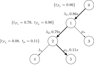
5.1 Example of a empirical generalized semi-Markov process . . . 58

5.2 Empirical generalized semi-Markov process of a task scheduler with uncer-tainty . . . 58

5.3 Performance and convergence evaluation of our method . . . 60

5.4 Statistical analysis of a land-satellite mobile communication for a high speed train . . . 61

5.5 Probabilistic distributions of high speed train fading and non-fading of satel-lite communication . . . 62

(12)

5.6 Event language specification of learned model of a high speed train . . . 63 5.7 Discrete state space partition of 11 second-order differential equations . . . 64 5.8 Stochastic automaton learned with our proposed method . . . 65 C.1 Examples of using SDES toolbox in Matlab . . . 76

(13)

List of Tables

4.1 Code lines analysis of SDES toolbox for Matlab . . . 53 5.1 The boundary values of discretization of several second-order equation

sim-ulations . . . 65 5.2 Estimated parameters of the learned (hundred) second-order simulations . . 65 A.1 Relations between truth/falseness of the null hypothesis and outcomes of

the test. . . 70

(14)

(15)

List of Algorithms

1 Scheduler estimator (SE) . . . 36

2 Probabilistic similarity of states (PSS) . . . 39

3 Similar function . . . 40

4 Deterministic mergefunction . . . 41

5 Estimation function . . . 43

(16)

(17)

Chapter 1

Introduction

Discrete event systems (DES) are actually a wide class of systems that are encountered daily. The canonical example is a simple queuing system with a single server. For ex-ample, consider a post office with only one employer, and therefore one queue for letters, packages, etc. The customers arrive the post office, deposit the goods in the queue, are attended by the postal worker, and then leave the post office. We can think of the ar-rival and departure of a customer as two separate events. There is no synchronization between the arrival and departure of customers, i.e. the two events just introduced are asynchronous and do not occur at the same time so this is clearly an example of a DES. Coping with asynchronous events is the major advantage of DES. Other examples of DES besides queuing systems include, computer systems, communication systems, manufactur-ing systems, traffic systems, database systems, software systems - telephony, and hybrid systems (hybrids between DES and continuous-variable dynamic systems (CVDS)).

This thesis explores an extension of DES with an emphasis on stochastic processes. This type of system is commonly called a stochastic discrete event system (SDES). When we talk about stochastic processes, we have to know that the dynamics of DES is described by a set of random variables (i.e., a stochastic process). For example, the arrival rate of customers at the post office or the risk that the post office is closed for some reason. These random variables have certain probabilistic distributions that can model the system behavior. We concern ourselves with how these probability distributions are obtained. These distributions are given by a collection of realistic measures to which we fit an analytic distribution function. This will be made due to a well established learning algorithm that accurately captures the timing of events from the real world, therefore there are no empirical assumptions.

(18)

1.1 The Problems

In this thesis, we consider one main problem and three secondary problems. The main problem is the learning of generalized semi-Markov processes (GSMP). The next prob-lem is to establish a relation between GSMP and SDES in order to verify them. The second secondary problem is to establish abstractions for continuous systems in order to be modeled as DES or SDES (respectively, non-stochastic and stochastically). The last problem is to apply stochastic and non-stochastic testing generation for the SDES such as perturbation model or classical unit testing suite. In the following lines, we shall describe these four problems in a more detailed manner.

− The learning of well defined stochastic processes has always been a great challenge. Although there exist complex models that are analytically intractable, actually there is a set of problems that were solved by the technique of model checking (more precisely statistical model checking). However, existing solutions assume that the acquisition of empirical models is enough. Today, we could safely say that they are not enough for most real systems like critical systems, due to its growing complexity. In this case, for the verification, only a model and a set of properties are needed to be able to determine whether the system satisfies some given property. Thus, verifying empirical models may not make sense. Solving the learning problem for a class of stochastic processes allows us to verify not only the model but to ensure some guaranties about the implementation and allows us to use that model for test generation.

− The relation between SDES and GSMP must be compatible (coincident). Thus, the GSMP has to be established as a more abstract model for SDES. With this, we can verify statistically SDES.

− Continuous variable dynamic systems are a class of systems that include all known dynamic systems defined by differential or difference equations. As we know, this type of systems require in many cases a lot of computational resources. At present, continuous systems run in discrete event platforms like a computer, for example, a satellite calculates its perturbations and corrections to maintain its trajectory. So, if a continuous system is executed as a discrete system, we can model it with some abstractions as a DES. There are many advantages. First, we can simulate systems with much less resources than those that are needed for continuous cases. Second, we can simplify (with abstractions) with a minor loss of precision. This is a vast problem that would require another new thesis. In this thesis we will address only

(19)

1.2. SUMMARY OF RESEARCH CONTRIBUTION 3

the preliminaries of the problem by defining and identifying the challenges to be addressed. Third, we can use DES easily to make its verification through the model checking technique and for test generation. Fourth, we can also use it for generation of perturbation models, for dynamic systems. Lastly, there exists a lot of simulators for discrete event systems, including parallel simulation.

− Testing is an essential methodology to target some parts of one system to find a set of problems/defects (bugs). The original challenge of this thesis was to derive a new methodology for test generation from stochastic models. The complex systems are not traceable to test all possible inputs. So, model testing generation requires a set of realistic models, otherwise we are running the risk of create many tests that are not time feasible (time-consuming and potentially expensive procedures). We shall discuss, in the next chapters, the problem of generating excessive test sets. A method to reduce it is using test generation based on realistic inputs, some that occurs in a realistic scenario shall also be discussed in this thesis.

1.2 Summary of research contribution

SDES are a large class of known stochastic systems with a good intuitive basis. At present, there are several learning algorithms that can be adopted for SDES. For instance, Sen et al. [2004b] has proposed learning the continuous-time Markov processes, but other processes or algorithms for a more general approach do not exist. However, there is no learning algorithm for stochastic systems that does not hold the Markov property. The generalized semi-Markov processes are a large class of stochastic processes that does not hold it. Obviously, this made this type of model more complex and analytically intractable. Hence, learning GSMP is statistically an ambitious due to its potentialities in this area.

We propose in this thesis a new and unique methodology for learning generalized semi-Markov processes that is the most extensive model when lifetimes can be governed by any continuous probabilistic distributions. As we know from classical Markov processes, the exponential distributions are not enough to model the lifetime of a product (e.g., a electronic component life) [Lu and Wang, 2008] or even a computer process [Harchol-Balter and Downey, 1997, Leland and Ott, 1986].

We propose an algorithm to learn generalized semi-Markov processes, that can be used for stochastic discrete event systems. We show with our experiments that this type of model is really capable and scalable. We can use it for analysis of an industrial system but also to verify or testing it.

(20)

have come out of our research efforts and is now available to the public 1_.

1.3 Overview of this thesis

This thesis is concerned with discrete event systems, in particular on stochastic extensions. Furthermore, it introduces the concept of a perturbation model for continuous systems. A comprehensive introduction to terminology, notation, and techniques that are used extensively throughout the thesis is given in chapter 2. It contains a brief overview on DES, stochastic processes, and SDES. Moreover, it presents some known common examples.

Chapter 3 provides the context for our research contribution with a discussion of related work in learning generalized semi-Markov processes, abstractions for continuous systems using the discrete event specification (DEVS) approach, probabilistic/statistical model checking, and test generation for stochastic processes.

We start in chapter 4 by introducing the notion of learning generalized semi-Markov processes. Some preliminary definitions are made in order to understand the terminologies that are made there. This work originated in an effort to develop a learning approach for SDES [de Matos Pedro et al., 2011]. We also describe the notion of abstraction for continuous systems and two approaches for statistical model-base test generation.

The evaluation of the learning algorithm is described in chapter 5. Three case stud-ies are studied. The first, consists on an empirical evaluation of the generalized-semi Markov processes learning algorithm. The second, a realistic case study for the analysis of availability from a communication between a satellite and a high-speed train. Lastly, an abstraction of a continuous system is made in order to be described and simulated as DES.

Finally, chapter 6 discusses directions for future work in continuous systems abstrac-tions and stochastic testing. For abstracabstrac-tions of continuous systems there is a need for applying this approach to stochastic polynomials or polynomial chaos. For testing it shall be adopted a full stochastic approach for creating a toolbox to test generation for SDES.

(21)

Chapter 2

Systems and models

In this chapter some basic concepts of system’s theory based on the definitions of Cassan-dras and Lafortune [2006] and Zimmermann [2007] shall be given. No detailed explana-tions about the concepts of state space, sample equation, sample path and feedback shall be given. We suppose that the reader is familiarized with those concepts, nevertheless, it should be suficient for the reader to use their intuition in order to understand them.

We begin our description of discrete event systems (DES’s) by first identifying their fundamental characteristics, and by presenting a few familiar examples of such systems. Lastly, we describe two extensions (deterministic and stochastic) of DES’s that will be used in the next chapters.

2.1 An introduction to discrete event systems

We shall now describe system in terms of a primitive concept like a set or a mapping. We provide three definitions about ”What is a system” as found in Cassandras and Lafortune [2006]:

− An aggregation or assemblage of things so combined by nature or man as to form an integral or complex whole.

− A regularly interacting or interdependent group of items forming a unified whole. − A combination of components that act together to perform a function not possible

with any of the individual parts.

In these definitions there are two salient features. First, a system is composed of a set of components, and second a system is associated with one function that presumably intends to perform something.

DES’s are a particular class of systems that are largely used in industry as pattern model Cassandras and Lafortune [2006]. So, when the state space of a system is naturally described by a discrete set like _{{0, 1, 2, ...}, and state transitions are only observed at}

(22)

discrete points in time, we associate these state transitions with events and talk about a DES.

Usually DES’s can be used as an hybrid model combined with continuous-variable dynamic systems (CVDS). The CVDS changes with measured quantities such as temper-ature, pressure and acceleration, which are continuous variables evolving over time. It is usually characterized by a continuous state space. So, in contrast to CVDS, DES’s evolves in a discrete state space, where at each transition there exists an associated event (i.e., an event-driven system).

2.1.1 The concept of event

The event is a primitive concept with a good intuitive basis. As Cassandras and Lafortune [2006] say we need to ”... emphasize that an event should be thought of as occurring instantaneously and causing transitions from one state value to another.”.

An event can be identified when a specific action occurs (e.g., a package arrived at a warehouse or a button is pressed), or it can be viewed as a spontaneous occurrence dictated by nature (e.g., a computer crash for whatever reason too complicated to figure out or a set of sensors that are unstable when temperature changes), or it can be viewed as a result of several conditions which are suddenly all met (e.g, the fluid level in a tank has just exceeded a given value or a warehouse that suddenly is full).

At this point, it is clear for us that DES’s are event-driven systems, they depend on discrete occurrences (i.e., something occurs due to an action, an event or something not well defined). Thus, we will introduce the informal definition of these systems and compare it with continuous systems which are guided by the time.

Event-driven systems and time-driven systems. In continuous-state systems the state generally changes as time changes. This is particularly evident in discrete-time models, where the clock is what drives a typical sample path. With every clock tick the state is expected to change, since continuous state variables continuously change with time. It is because of this property that we refer to such systems as time-driven systems. In this case, the time variable (t in continuous time or k in discrete time) is a natural independent variable which appears as the argument of all input, state, and output functions.

In discrete-state systems, we say that the state changes only at certain points in time through instantaneous transitions. To each such transition we can associate an event. However, the description of the timing mechanisms based on which events take place before it can be triggered is missing. We describe it in detail in section 2.2.

(23)

2.1. AN INTRODUCTION TO DISCRETE EVENT SYSTEMS 7

2.1.2 The model characterization and its abstractions

The event-driven property of DES was discussed in the previous section. It refers to the fact that the state can only change at discrete points in time, which physically correspond to occurrences of asynchronously generated discrete events. From a modeling point of view, this has the following implication. If we can identify a set of events any one of which can cause a state transition, then time no longer serves the purpose of driving such a system and may no longer be an appropriate independent variable. Thus, the DES satisfies the following two properties:

1. The state space is a discrete set.

2. The state transition mechanism is event-driven.

However, according to these properties and as described by Cassandras and Lafortune [2006] DES’s are informally described by the definition 1. So, the state space is some discrete set X ={s1, s2, ..., sn}, where X is a set of finite states that have the state s1, s2,

..., snand n is a finite size of state space (see definition 2).

Definition 1. A Discrete Event System (DES) is a discrete-state, event-driven system, that is, its state evolution depends entirely on the occurrence of asynchronous discrete events over time.

Definition 2. The state space of a system, usually denoted by X, is the set of all possible states that the system may take.

The sample path1 _{can only transiting from one state to another whenever an event occurs.}

Note that an event may take place, but not cause a state transition. For example when one event occurs at state s2 and goes to the same s2state (i.e., an arc or a loop transition).

It is often convenient to represent a DES sample path as a timing diagram (timeline) with events identified by vertical dashed lines at the times they occur, and states shown in between events like the figure 2.3.

DES’s have a set of models available for the most diverse systems. So, due to this, we describe below some abstractions for different DES’s. Note that DES’s may be viewed as an event-language or even just a language.

The abstractions of DES’s. Languages, timed languages, and stochastic timed lan-guages represent the three levels of abstraction at which DES’s are modeled and studied: untimed (or logical), timed, and stochastic. We describe in the following sections (see

1_{The sample path is one simulation (sample execution) of a DES; It identifies the behavior of DES’s} over time, where the time instants are discrete steps in the state space.

(24)

sections 2.2 and 2.4) the timed automaton and stochastic timed automaton, which are two abstract models for describing DES’s.

Remark 2.1. One should not confuse discrete event systems with discrete-time systems. The class of discrete-time systems contains both CVDS and DES’s. In other words, a DES may be modeled in continuous or in discrete time, just like a CVDS can.

2.1.3 Hybrid models

Systems that combine time-driven with event-driven dynamics are referred to as hybrid systems. Recent years have seen a proliferation of hybrid systems largely due to the embedding of microprocessors (operating in event-driven mode) in complex automated environments with time-driven dynamics; examples arise in automobiles, aircraft, chemical processes, heating, ventilation, and air-conditioning units in large buildings, etc.

We do not describe here formally any definition for a hybrid model, therefore, we will try to deduce one perturbation model from a continuous variable system based on other abstractions such as differential equations and difference equations.

A more close example of a hybrid system will be shown later in section 4.4, where a perturbation model from an inverted pendulum is described and modeled.

2.1.4 Examples

The subtleties of DES’s were described in the previous sections. There are many common examples such as: a computer system crashing due to periodical bugs that obligate its watchdog to reboot it or even a bottle filling line of an industry (a hybrid industrial system). Here we shall discuss in detail one practical example of a warehouse system manager.

The model that we will describe is quite misunderstood from a mathematics point of view principally due to discontinuities (there is more time when nothing occurs than when sometimes does occurs). Now, in this sense what we need to explain is that there are other models with better abstractions, which we will explain in the next sections. They are timed automata (see section 2.2) and stochastic timed automata (see section 2.4).

Example 2.2. Consider a warehouse containing packages of goods from a shipping company (a particular case of the example provided by Cassandras and Lafortune [2006]). When a new package is received by the shipping company, this represents an arrival event at the warehouse and when the shipping company dispatches the package it is a departure event. So, a truck periodically delivers and loads up a certain number of products, which are thought of as departures from the warehouse (figure 2.1). With this model we can

(25)

2.1. AN INTRODUCTION TO DISCRETE EVENT SYSTEMS 9

Arrival

Departure

Figure 2.1: A warehouse of a shipping company depicted in a simple diagram of input of goods and the output of packages. The packages arrive at the warehouse as arrival events and the departures of packages from warehouse as departure events. Thus, the DES is defined by the number of packages at the warehouse (the state space) and the actions triggered by this two events.

check if the storage capacity of a particular warehouse located in Lisbon is enough or not. We can analyze how many packages have arrived and departed at one time instant of the system or also over a long run execution.

We can analyze the warehouse system as a queuing system. This system can be modeled as a DES where the number of packages is determined by the state space of the system. Thus, we define x(t) to be the number of products at time t, and define an output equation for our model to be y(t) = x(t). For instance supposing that at most ten packages can be stored, we will have a system with discrete state space X =_{{1, 2, 3, 4, ..., 10}.}

We define two binary functions u1 and u2 that correspond to the arrival event and

departure event to indicate that in time t an event has occurred,

u1(t) =

 



1 If a package arrives at time t

0 otherwise (2.1) and u2(t) =   

1 If a package departs at time t

0 otherwise (2.2)

The sequence of time instants when u1(t) = 1 defines the schedule of package arrivals

at the warehouse. Similarly, the sequence of time instants when u2(t) = 1 defines the

schedule of package departures from the warehouse.

We next describe the simplifications that we have assumed for the model. First, the warehouse have space for at most of ten packages and its storage capacity is reached at ten packages. Next, the loading of the truck takes zero time. Then, the truck can only take away a single product at a time. Lastly, a package arrival and a package departure never take place at exactly the same instant, that is, there is no t such that u1(t) = u2(t) = 1. In

order to derive a state equation for this model, let us examine all possible state transitions we can think of:

(26)

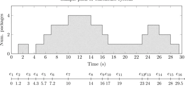
0 2 4 6 8 10 12 14 16 18 20 22 24 26 28 30 0 2 4 Time (s) Num. pac kages

Sample path of warehouse system

0 e1 1.2 e2 3 e3 4.3 e4 5.7 e5 7.2 e6 10 e7 14 e8 16 e9 17 e10 19 e11 23 e12 24 e13 26 e14 28 e15 29.5 e16

Figure 2.2: A sample path of the warehouse system with an event timeline on bottom.

1. u1(t) = 1, u2(t) = 0. This simply indicates an arrival at the warehouse at time

instant t. As a result, x(t) should experience a jump of +1, if x(t)≤ 10.

2. u1(t) = 0, u2(t) = 1. This means a truck is present at time t, and we should reduce

the warehouse content by 1. However, there are two sub-cases. If x(t) > 0, then the state change is indeed−1. But if x(t) = 0, the truck finds the warehouse empty and the state does not change.

3. u1(t) = 0, u2(t) = 0. Clearly, no change occurs at time t.

Let t+ _{denote the time instant just after t. With this notation, based on the}

observa-tions above we can describe it with the following state equation:

x(t+) =        x(t) + 1 if (u1(t) = 1, u2(t) = 0, x(t)≤ 10) x(t)_{− 1} if(u1(t) = 0, u2(t) = 1, x(t) > 0) x(t) otherwise (2.3)

A typical sample path of this system is shown in figure 2.2. In this case, u1(t) = 1 (i.e.,

packages arrive) at time instants t1, t2, t3, t5, t6, t12, and t13, and u2(t) = 1 (i.e., a truck

arrives) at time instants t4, t7, t8, t9, t10, and t11. Note that even though a truck arrival

takes place at time t11, the state x(t) = 0 does not change, in accordance with figure 2.2.

Remark 2.3. The equation 2.3 is an illustration of many situations we could be encoun-tering on the common DES. This warehouse system is modeled as a stack, therefore the mathematical model is rather informal and it is not the most interesting model. In most of the time nothing happens due to the discontinuities of the functions u1 and u2.

(27)

2.2. TIMED AUTOMATA 11

2.2 Timed automata

An automaton is a model that is capable of representing a language (i.e., a sequence of input symbols) according to well-defined rules. The simplest way to present the notion of automaton is to consider its representation as a directed graph, or state transition diagram. So, we present here the definitions of the deterministic timed automaton (DTA) followed by the definition of the clock structure. Lastly, we expose a practical example of a simple DTA.

Definition 3. The deterministic timed automaton is a six-tuple M = (_{X , E, f, Γ , x}0, V ),

where

X is a countable state space,

E is a countable event set,

f :_{X × E → X} is a state transition function and is generally a partial function on its domain,

Γ :_{X → 2}E is the active event function (or feasible event function); Γ (x ) is the set of all events e for which f (x, e) is defined and it is called the active event set (or feasible event set),

x0 is the initial state, and

V =_{vi : i∈ E} is a clock structure.

Having presented the definition of DTA we can make some remarks about it, however we focus here only on the essential. Our remarks (see Cassandras and Lafortune [2006]) are: − The functions f and Γ are completely described by the state transition diagram of

the automaton.

− The automaton is said to be deterministic because f is a function from X × E to X , namely, there cannot be two transitions with the same event label out of a state. − The fact that we allow the transition function f to be partially defined over its

domain _{X × E is a variation over the usual definition of automaton in computer} science literature that is quite important in DES’s theory.

− Formally speaking, the inclusion of Γ in the definition of M is superfluous in the sense that Γ is derived from f . One of the reasons why we care about the contents of Γ (x ) for state x is to help distinguish between events e that are feasible at x but cause no state transition, that is, f (x, e) = x, and events e0 that are not feasible at x, that is, f (x, e0) is not defined.

− The event set E includes all events that appear as transition labels in the state tran-sition diagram of automaton M . In general, the set _{E might also include additional} events, since it is a parameter in the definition of M . In other words, this can be composed by a parallel composition.

(28)

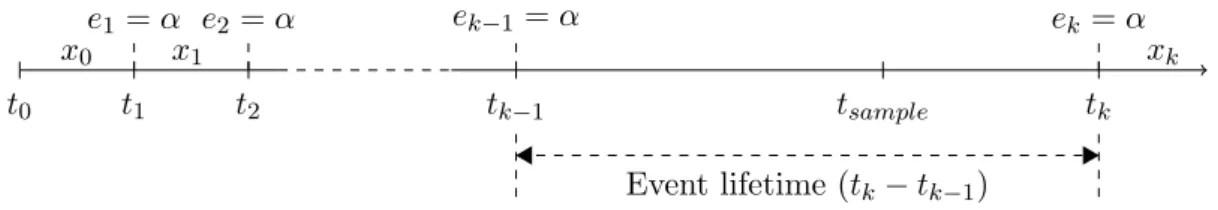
t0 t1 e1 = α t2 e2= α x0 x1 xk t_k−1 ek−1 = α tk ek= α tsample Event lifetime (tk− tk−1)

Figure 2.3: The timeline of a simple DES with one α event is depicted. The lifetime of an event

of one DES is the time between two consecutive identical events, in this example, around tsample

have a lifetime of tk− tk−1.

− The V clock structure has one clock associated for each event. Each clock is made by a composition of an ordered set of fixed clock values. We formally describe it in the following section.

2.2.1 The clock structure

We introduce here the key ideas of timed DES’s. As we have previously seen a simplified DES is a system composed of a finite set of statesX , and a finite set of events E. It has one transition function f , that given an event knows what is the next state and an activation function Γ that knows what events are active in a given state. So, knowing all of this a clock structure is needed in order to drive the time of each event.

Example 2.4. (A DES with a single α event.) LetE = {α}, and Γ (x ) = {α} for all x ∈ X . A simulation of this system always produces the same output. So, the generated path, an event sequence, is denoted by p = (e1, e2, e3, ..., en), ek = α, for each k = {1, ..., n}.

The time instant associated with the kth _{event is denoted by t}

k, k = {1, 2, ..., n}. The

length of the time interval defined by two successive occurrences of the event is called a lifetime as we can see in the timeline of the figure 2.3. We denote vk, the lifetime of the

kth event. Thus, we define vk= tk− tk−1 ∈ R+, for each k.

The evolution of this system over time can be described as follows. At time tk−1, the

kth event is said to be activated or enabled, and is given a lifetime vk. A clock associated

with the event is immediately set at the value specified by vk, and then it starts ticking

down to 0. During this time interval, the kthevent is said to be active. The clock reaches zero when the lifetime expires at time tk = tk−1 + vk. At this point, the event has to

occur. This will cause a state transition. The process then repeats with the (k + 1)th

event becoming active.

To introduce some further notation, let tsample be any time instant, not necessarily

associated with an event occurrence. Suppose that tk−1 ≤ t ≤ tk. Then t divides the

(29)

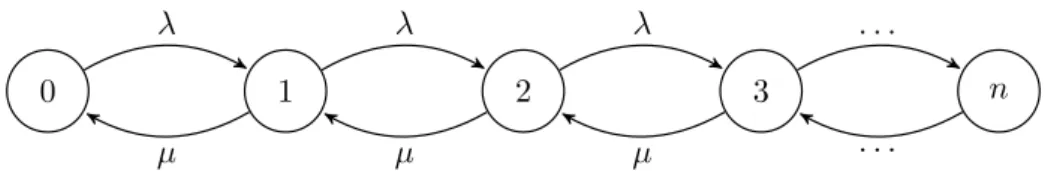
2.2. TIMED AUTOMATA 13 0 1 2 3 n λ λ λ . . . . . . µ µ µ

Figure 2.4: A discrete event system of the D/D/1/n stack.

or residual lifetime of the kth event, and zk = t− tk−1 is called the age of the kth event.

It is obvious that vk = zk + yk. It should be clear that a sample path of this DES is

completely specified by the lifetime sequence (v1, v2, ..., vn). This is also referred to as the

clock sequence of event α.

Example 2.5. (A simple timed automaton - a stack model with n elements.) This model is a more interesting DES. It has concurrence between two events. Let the event set be _{E = {λ, µ}. The state transition diagram of the figure 2.4 depicts a stack model} with n states. The set of nodes is the state set of the automation, _{X = {0, 1, 2, 3, ..., n}.} The labels of the transitions are elements of the event set (alphabet) E of the automaton. The arcs in the graph provide a graphical representation of the transition function of the automaton, which we denote as f :X × E → X :

f (0, λ) = 1

f (1, λ) = 2, f (1, µ) = 0 f (2, λ) = 3, f (2, µ) = 1

...

f (n, µ) = n_{− 1}

The notation f (1, λ) = 2 means that if the automaton is in state 1, then upon the oc-currence of event λ, the automaton will make an instantaneous transition to state 1. The cause of the occurrence of event λ is irrelevant; the event could be an external input to the system modeled by the automaton, or it could be an event spontaneously generated by the system modeled by the automaton. So, if model is in state 1 that has f (1, λ) = 2 and f (1, µ) = 0. At this point the system can trigger one of those events. These events compete with each other one to trigger the event with less holding time. For instance, if vλ = (1, 10, 30, ...) and vµ = (2, 5, 32, ...) we begin by making a transition λ (the only

possible transition) with time vλ,1, and next compare the clock value of vλ,2 and vµ,1when

µ event wins. Then, the automaton will make an instantaneous transition to state 1 and trigger the event λ with a holding time of vλ,2, and so on. It should be clear that a sample

(30)

2.3 Stochastic process basics

In this section, we briefly introduce the concept of stochastic process always followed by practical examples.

A stochastic process is simply a collection of random variables indexed through some parameter, which is normally thought of as time. For example, suppose that Ω = {IDLE, CRASHED} is the sample space for describing the random state of a com-puter system (like the last one). By mapping IDLE into 0 and CRASHED into 1 we may define a random variable X(ω), ω ∈ Ω, which takes the values 0 or 1. Thus, X(ω) = 1 means the computer system is CRASHED, and X(ω) = 0 means the computer system is IDLE. Next, suppose that we describe the state of the computer system over time as discrete steps. Let k = 1, 2, 3, ... be the index of the time (i.e., seconds, hours, days, etc...). Thus, X(ω, k) is a random variable describing the state of computer system on the kth time step. The collection of random variable _{{X(ω, 1), X(ω, 2), ..., X(ω, k), ...} defines a} stochastic process.

Definition 4. A stochastic or random process X(ω, t) is a collection of random variables indexed by t. The random variables are defined over a common probability space (ω, E, P ) with ω _{∈ Ω. The variable t ranges over some given set T ⊆ R.}

The probability space is defined by the 3-tuple (ω, E, P ), where ω determine the sample space, which is the set of all possible outcomes, E is a set of events, where each event is a set containing zero or more outcomes, and P the probabilities of the events.

The mathematical abstractions for DES’s with stochastic clock structure (see later) is a stochastic process, which is formally a collection of random variables (as we have seen above) that we denote by _{{X(t) | t ∈ T}, where t is the time indexing. The parameter t} may have a different interpretation in other environments. Index set T denotes the set of time instants of observation. The set of possible results of X(t) is called state space of the process (a subset of R), and each of its values corresponds to a state.

Stochastic processes are characterized by the state space and the index set T. If the state space is discrete (countable), the states can be enumerated with natural numbers and the process is a discrete-state process or simply a chain. T is then usually taken as the set of natural numbers N. Otherwise, it is called a continuous-state process. Depending on the index set T the process is considered to be discrete-time or continuous-time. Four combinations are obviously possible. In our setting of stochastic discrete event systems, we are interested in systems where the flow of time is continuous (T = R+0) and the state

space is discrete. The stochastic process is thus a continuous-time chain and each X(t) is a discrete random variable.

(31)

2.4. STOCHASTIC TIMED AUTOMATA 15

Now, we describe the inherent properties of a Markov process. They are the following two properties:

Property 2.6. the future state only depends on the current state and not on the states history (no state memory is needed )

Property 2.7. the inter-event time in the current state is irrelevant in determination of the next state (no age memory is needed )

A discrete-state stochastic process_{{X(t)|t ∈ T} is called a Markov chain if its future} behavior at time t depends only on the state at t.

P{X(tk+1) = nk+1|X(tk) = nk, ..., X(t0) = n0} = P {X(tk+1) = nk+1|X(tk) = nk} (2.4)

Processes that hold a Markov property are easier to analyze than more general pro-cesses because information about the past does not need to be considered for the future behavior. Markov chains can be considered in discrete or continuous time, and are then called discrete-time Markov chain (DTMC) or continuous-time Markov chain (CTMC). From the memoryless2 property of a Markov process it immediately follows that all inter-event times must be exponentially (CTMC) or geometrically (DTMC) distributed. Dif-ferent relaxations allow more general times. Examples are semi-Markov processes [Barbu and Limnios, 2008] with arbitrary distributions but solely state-dependent state transitions and renewal processes that count events with arbitrary but independent and identically distributed interevent times.

A generalized semi-Markov process (GSMP) [Glynn, 1989] allows arbitrary inter-event times like semi-Markov process. The Markov property of state transitions depending only on the current state is achieved by encoding the remaining delays of activities with nonmemoryless delay distributions in the state, which then has a discrete part (the system states) and a continuous part that accounts for the times of running activities.

2.4 Stochastic timed automata

Stochastic timed automata (STA’s) according to the definition of timed automata have changes on clock structure and a little difference in the transition function. Broadly, the stochastic automaton is an automaton with stochastic clocks.

We begin by adopting a random variable notation to define the clock structure of timed automata as stochastic clocks: X is the current state; E is the most recent event (causing

2_{The memoryless is a property that some random distributions satisfies. The exponential distributions} of non-negative real numbers and the geometric distributions of non-negative integers.

(32)

the transition into state X); T is the most recent event time (corresponding to event E); Ni is the current score of event i; and Yi is the current clock value of event i. As in the

deterministic case, we use the prime (’) notation to denote the next state X0, triggering event E0, next event time T0, next score of i, N_i0, and next clock of i, Y_i0.

Besides the stochastic clock structure specification, there are two additional proba-bilistic features:

− The initial automaton state x0 may not be deterministically known. In general, we

assume that the initial state is a random variable X0. What we need to specify then

is the probability mass function (pmf) of the initial state

p0(x) = P [X0= x], where x∈ X (2.5)

− The state transition function f may not be deterministic. In general, we assume that if the current state is x and the triggering event is e0, the next state x0 is probabilistically specified through a transition probability3

p(x0; x, e0) = P [X0= x0_{|X = x, E}0 = e0], where x, x0 _{∈ X , e}0_{∈ E} (2.6) A timed automaton equipped with a stochastic clock structure (see section 2.4.1), an initial state cumulative distribution function, and state transition probabilities defines a Stochastic Timed Automaton, as defined below.

Definition 5. A Stochastic Timed Automaton is a six-tuple M = (X , E, Γ , p, p0, G)

where

X is a countable state space,

E is a countable event set,

Γ(x ) is a set of feasible or enabled events, defined for every x∈ X , with Γ (x )⊆ E,

p(x0; x, e0) is a state transition probability, defined for every x, x0 _{∈ X} and e0 ∈ E, and such that p(x0_{; x, e}0_{) = 0,} _∀e0 _{∈ Γ (x ),}_/

p0(x) is the pmf P [X0= x], x∈ X , of the initial state X0, and

G =_{Gi: i∈ E} is a stochastic clock structure.

The automaton generates a stochastic state sequence_{X0, X1, ...} through a transition

mechanism (based on observations X = x, E0 = e0): X0 = x0 with probability p(x0; x, e0) and it is driven by a stochastic event sequence _{E1, E2, ...} generated through

E0 = arg min

i∈Γ (X ){Yi} (2.7)

3_{Note that if e}0 /

(33)

2.4. STOCHASTIC TIMED AUTOMATA 17

with the stochastic clock values Yi, i∈ E, defined by

Y_i0 =    Yi− Y∗ if i6= E0 and i∈ Γ (X ) Vi,Ni+1 if i = E0 or i /∈ Γ (X ) i∈ Γ (X0) (2.8)

where the interevent time Y∗ is defined as Y∗ = min

i∈Γ (x ){Yi} (2.9)

the event scores Ni, i∈ E, are defined through

N_i0 =    Ni+ 1 if i = E0 or i6= Γ (X0) Ni otherwise i_{∈ Γ (X}0) (2.10) and Vi,k ∼ Gi (2.11)

where the tilde (∼) notation denotes ”with distribution”. In addition, initial conditions are: X0 ∼ p0(x), and Yi = Vi,1 and Ni= 1 if i∈ Γ (X0). If i /∈ Γ (X0), Yi is undefined and

Ni = 0.

Having presented the formal definition of stochastic timed automaton we need to make some remarks about comparison with definitions of the timed automaton. The transition function f is replaced by the probabilistic transition function p (the transition is made with uncertainty), x0 the initial state is replaced by p0 the probabilistic mass function

(the initial state is given by this function; it can start from a different set of states given by the pmf ), and lastly the main difference is that the stochastic automaton have G the stochastic clock structure instead of the V simple structure of events lifetime.

2.4.1 The stochastic clock structure

The clock structure of the stochastic timed automaton is defined according to definition 6. The stochastic process generates the lifetime sequences for each event given by Vi,k. The

clock structure of the timed automaton is the same of the used in this definition, but the difference is that it is governed by a stochastic process.

Definition 6. The stochastic clock structure (or timing structure) associated with an event set _{E is a set of distribution functions}

G =_{Gi: i∈ E} (2.12)

characterizing the stochastic clock sequences

(34)

2.5 The stochastic discrete event system

A stochastic discrete event system (SDES), according to Zimmermann [2007], is a tuple SDES = (SV, A, S, RV ) describing the finite sets of state variables SV and actions A together with the sort function S. The reward variables RV correspond to the quantitative evaluation of the model.

− S is a function that associates an individual sort to each of the state variables SV and action variables V ars in a model. The sort of a variable specifies the values that might be assigned to it. We will not specify here the type system, which we assume as implicit. We will present a simple example (see later) to understand better how the system behaves. The variable types and operations can be described by the semantics of the event language in the appendix B.

− SV is the finite set of n state variables, SV = {sv1, ..., svn}, which is used to capture

states of the SDES.

− A denotes the set of actions of a SDES model. They describe possible state changes of the modeled system. An action a_{∈ A of a SDES is composed of a set of attributes} that we are not describe here (please consider Zimmermann [2007]).

− RV is the notion of a quantitative evaluation of SDES called as reward variable. It is used as a set of variables to the analysis of the SDES (i.e., performance analy-sis, produce documents for documentation purposes, and verification). This is one feature that can be coupled for any DES therefore we will not describe it here. 2.5.1 Inclusion between stochastic timed automata and discrete event

systems

The SDES definition comprises state variables, actions, sorts, and reward variables.

SDES = (SV, A, S, RV ) (2.14)

In order to capture a stochastic automaton as defined in the previous section these variables are set in the following manner. There is exactly one state variable sv, whose value is the state of the automaton. The set of state variables SV has therefore only one element.

SV =_{sv} (2.15)

The set of SDES actions A is given by the events of the automaton.

(35)

2.5. THE STOCHASTIC DISCRETE EVENT SYSTEM 19

The sort function of the SDES maps the state variable to the allowed values, i.e., the state space of the automaton. As there are no SDES action variables necessary, no sort is defined for them.

S(sv) =_X (2.17)

The set of all possible states in SDES and in STA is obviously equal. The condition function also is always true, because all states in _{X are allowed. The initial value of the} state variable is directly given by the initial state of the automaton. The actions of the SDES correspond to events of the stochastic automaton.

The remaining concepts and details that are interesting but not relevant for this work are left to the reader. For more details see for instance Zimmermann [2007].

2.5.2 The generalized semi-Markov process

A stochastic timed automaton is used to generate the stochastic process {X(t)}. This stochastic process is referred to as a generalized semi-Markov process (GSMP).

Definition 7. A Generalized Semi-Markov Process (GSMP) is a stochastic process_{X(t)} with state spaceX , generated by a stochastic timed automaton (X , E, Γ , p, p0, G).

The GSMP simulation

The simulation concepts introduced by Ross [2006] and Banks [1998] shall now be described as well as the algorithms. We focus in particular on the simulation of generalized semi-Markov processes [Asmussen and Glynn, 2007].

Let us see the following example in order to understand the concept of simulation of a GSMP, its scheduler behavior, and its event competition.

Example 2.8. Given the M/M/1/n stack model (notation according to Kendall [1953]) of figure 2.5 that has _{E = {λ, µ}, X = {0, 1, 2, 3, ..., n} the discrete state space, and} Γ(0 ) ={λ}, Γ (1 ) = {λ, µ}, ..., Γ (n − 1 ) = {λ, µ}, Γ (n) = {µ}. As was described in the last sections, the behavior of the DES is that the events compete each other to trigger the event with the minimal time. So, with that in mind and looking to the timeline of the figure 2.6, that is one simulation of the stack model, we can view this event competition. The shadowing below the arrows is the more probable lifetime given by the distributions related to λ and µ events with high probability (black) and with low probability (gray). Notoriously, we can view after the first triggered event λ that at each discrete step the selection of the triggered events is the minor value of the two λ and µ events. The behavior is the same as DES but with stochastic clocks that have uncertainty in time duration.

(36)

0 1 2 3 n λ λ λ . . . . . . µ µ µ

Figure 2.5: The stochastic discrete event system of the M/M/1/n stack is depicted.

λ µ λ µ λ µ λ λ µ λ µ 1.0 2.0 3.0 4.0 5.0 6.0 0.0 0 1 2 1 2 3 2 3 e1= λ e2= λ e3= µ e4= λ e5= λ e6= µ e6= λ

Figure 2.6: The stochastic timeline of the M/M/1/n stack is depicted.

However, there is a big difference, that is each simulation has an uncertainty in the output. Now, the events are not governed by the simple structure of static lifetimes but guided by stochastic clocks that generate, according to this, the samples that is one lifetime (as we can see the shadowing bars).

We can see two type of events, λ and µ, which can be marked as active event or inactive depending on the present state. Thus, an active event can be an old clock or a new clock, and conversely an inactive event has an inactive clock. An old clock is achieved by the subtraction of the clock values of the triggered events until this old clock is triggered, i.e., it is assigned a original value minus every clock values that are triggered until then.

The definition of the inactive clocks, the new clocks and the old clocks is given by

C(en, i) =−1, en∈ E(S/ i)

C(en, i) =F(·, Si, Si−1, en), en∈ N(Si, Si−1, e)

C(en, i− 1) − C(e∗i−1, i− 1) = C(en, i), en∈ O(Si, Si−1, e)

(2.18)

where n is the number of events, i is the ith_{steps of simulation, and}_{F is a probabilistic}

distribution function. Therefore, the E(s) is a function of a set of active events in a state s, and N (s, s0, e) is the function of new clock in respect to an event and a transition to

(37)

2.5. THE STOCHASTIC DISCRETE EVENT SYSTEM 21

the s0 state to s. Consequently, we define the en ∈ O(Si, Si−1, e) based on the premise

en∈ N(S/ i, Si−1, e) and en∈ E(Si).

In this chapter we have reviewed the basic principles of DES and SDES as well as the specification of stochastic processes. However, an algorithm that estimates the scheduling of GSMP is needed in order to solve the learning methodology in a complete way. In the next chapter we shall review the state of the art concerning learning stochastic systems and this will serve as foundation for the specification of a new learning algorithm for GSMP and its abstraction for continuous systems.

(38)

(39)

Chapter 3

Related work

In the previous chapter we have given the main definitions and the essential background necessary to understand the concept of timed automaton, stochastic automaton, DES and SDES. In this chapter we review the state of the art of stochastic model learning, . In particular we shall concentrate on: learning generalized semi-Markov chain (see section 3.1), its abstractions for continuous systems including other approaches (see section 3.2), and two approaches that can verify and test stochastic models (see section 3.3 and 3.4). Not that this related work is centered around the development of the basic ideas of learning, verifying, and testing.

We begin with reviewing the learning algorithms for a set of stochastic models like probabilistic/stochastic automata (that identify a stochastic language), the discrete-time and continuous-time Markov chains, and briefly the hidden Markov chains. Next, a few other approaches to abstract the continuous systems are discussed. This is followed by re-cent work about statistical model checking, on which tools have been developed that allow the verification of the learned models. Lastly, we describe the existent testing methods that are able to test stochastic models.

However, since the models (automata, Markov chains, etc) are directly related with DES or SDES we could use probabilistic/statistical model-checkers to check them. More-over we can generate a set of tests from these models, unit tests or stochastic tests. Also, the learning approach can be used to learn models, which can then be verified and tested.

3.1 Learning stochastic and probabilistic models

Learning algorithms are widely used for system analysis and system modeling. As we have said in the previous chapter, the verification and test of stochastic systems is our main goal. Machine learning solved several problems but in most cases does not ensure

(40)

its reliability. So, today some models have scarce reliability. Here we discuss some proba-bilistic/stochastic learning methods where our goal is to use statistical model checking to verify it.

The stochastic models are used for reliability and performance analysis of a set of com-plex systems. As we have presented in the previous chapter various models are available. Now, we describe some related algorithms for its learning. Carrasco and Oncina [1994] introduced the criterion of learning stochastic regular grammars. They proposed an al-gorithm based on state merging to learn a probabilistic automaton. This method begins by the construction of one prefix tree from a set of output sequences provided by one implementation (called sample executions). Next, they established a well defined stable relation (the state equivalence) to merge equal states. This process produces a stochastic automaton that recognize a stochastic language. It is based on the beginning principle of language identification in the limit which was introduced by Gold [1967]. He also proved that regular languages cannot be identified if only text is given, but they can be identified if a complete presentation is provided (i.e. ”Is the information sufficient to determine which of the possible languages is the unknown language?”). Later, Carrasco and Oncina [1999] propose the same solution but in polynomial time.

A more close method is the work developed by Kermorvant and Dupont [2002]. They present a new statistical framework for stochastic grammatical inference algorithms based on a state merging strategy. They use the multinomial tests for establishing the equivalence relation between the states. Their approach has three advantages. First, the method is not based on asymptotic results, and thus small sample case can be specifically dealt with. Second, all the probabilities associated to a state are included in a single test (chi-square test - X2_{). Third, a statistical score is associated to each possible merging operation and}

can be used for best-first strategy.

Given the good results of the learning probabilistic automatons, Sen et al. [2004b] propose a new extension to learn the continuous-time Markov chains. Their learning algorithm consists in learning a model from an edge labeled continuous-time Markov chain (see section 3.3). Moreover, with this method we can use the learned model from a set of practical systems (e.g, the industrial systems, the avionic systems, and the automobile systems) as the input model for a set of available tools. These tools allow the analysis, verification and testing of Markov chains.

Another closely related work is proposed by Wei et al. [2002]. They propose a method to learn continuous-time hidden Markov chains and also propose the acquisition process with fixed length of sample executions (the sample executions have a finite and a static length defined before all the learning process). This causes a serious trouble in the learning

(41)

3.1. LEARNING STOCHASTIC AND PROBABILISTIC MODELS 25

process if the specified size is not large enough to learn the model, which is known as the problem of insufficient training data. The learning theory shows that the values computed by the training algorithms converge to the correct probabilities if the amount of training data tends to infinite. In practice an existing bias is observed. Which one depends on the number of training samples and on the length of the samples. When the length increases, the likelihood of a given sequence decreases.

In the following, we explain in detail the learning approaches which will form the basis of the next chapter.

3.1.1 Learning continuous-time Markov chains

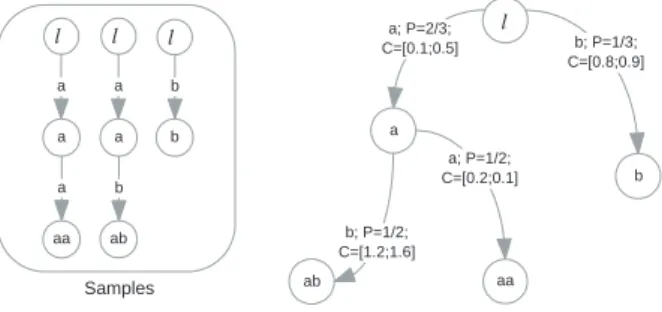
We explain here some details of the learning methodology proposed by Sen et al. [2004b]. They proposed an algorithm also based on state merging paradigm introduced by Carrasco and Oncina [1994]. The prefix tree is constructed given a set of sample executions. A prefix tree has two fields coupled to each node, which are the following: expectation value to each transition branch, and clock samples to each label in a prefix tree node. For example, figure 3.1 illustrates a prefix tree with five nodes generated by three paths. It has the transition labels{a, b}, P that is the expected value to the respective branch, and C the clock samples from transitions.

a b ab a; P=2/3; C=[0.1;0.5] b; P=1/2; C=[1.2;1.6] b; P=1/3; C=[0.8;0.9] l a ab b a b b l l aa a; P=1/2; C=[0.2;0.1] a aa a a l Samples

Figure 3.1: Example of a prefix tree constructed from three sample executions. It has five nodes and four transitions each one annotated.

A prefix tree is used to find similar states which is the essence of this state merge paradigm. When two similar states are found, they should be merged to give rise to a new model. This process is made recursively for each node in the prefix tree. After that process one generates a Markov chain, which in this case is an edge labeled Markov chain. As we have referred, this is an extension of a known continuous-time Markov chain. This chain has one label (an identification symbol) coupled to each transition and it solves the nonexistence of transition symbol in CTMC.

The proof of concept in this case is an indispensable task. Thus, Sen et al. [2004b] demonstrate that given a structurally complete sample to his learning algorithm, in the

(42)

limit (as sample executions grows to infinite), the learned model is similar or equal to the original model.

There is other approach that we will not explain here that is based on empirical rules to learn and classify Markov chains [Lowd and Davis, 2010].

3.1.2 Learning hidden Markov chains

The hidden Markov chains [Barbu and Limnios, 2008] have become increasingly popular in the last several years, for different reasons according to Rabiner [1990]. There are two strong reasons why this has occurred. First the models are very rich in mathematical structure and hence can form the theoretical basis for use in a wide range of applications. Second the models, when applied properly, work very well in practice for several important applications.

We pointing here some related work about hidden Markov chains in order to know how to learn the observable process.1 _{Rabiner [1990] proposes a method to learn hidden}

Markov models in order to provide a method for voice recognition. Wei et al. [2002] also proposes a method to learn continuous-time hidden Markov chains for modeling network performance.

However, our objective here is to make it known that there are other types of models (with a hidden part) that could be verified or tested.

3.1.3 Learning stochastic languages with artificial neural networks

The artificial neural network (ANN) introduced by McCulloch and Pitts [1988] describes a formal approach of the human brain. The ANN aims to emulate the human thinking process, and it is constructed by a binary network of neurons in which each neuron is composed by one activation function and some synopses. The synopses are the input signals for the activation functions of neuron, which are provided by other connected neurons in the ANN.

Carrasco et al. [1996] have introduced the criterion of learning stochastic grammars, which are mentioned in the previous chapter, but also another learning method based on ANN. In his paper he affirms that the generalization ability of their method is acceptable, and that the second-order recurrent neural network may become a suitable candidate for modeling stochastic processes. However, he does not propose an analysis of his approach, and does not guarantee some important properties of the ANN method, which are ensured in the method based on MCs.

(43)

3.2. DISCRETE EVENT SYSTEMS SPECIFICATION 27

The ANNs models have advantages and disadvantages over the MCs. The ANNs have a variety of learning methods, which allows to obtain easily a reasonable model. However, in many cases the reliability of this model is unobtainable, and an analysis of an ANN is in-tractable, due to its complexity and non linearity. The stochastic models are clearly better in analysis and verification. This is due mainly to the developed statistical/probabilistic model checking tools (see 3.3).

The stochastic solution is more expensive to calculate, nevertheless verifying properties in learned models is more efficient. Considering the advantages and disadvantages of the various approaches stochastic models are overall the best option.

3.2 Discrete event systems specification

The discrete event system specification (called DEVS) is a specification that it is commonly used in industry. DEVS is a modular and hierarchical formalisms for modeling and ana-lyzing general systems (Wainer [2009] has written a very interesting book about DEVS). This systems are described by: discrete state systems, continuous state system that can be described by differential equations, and hybrid state systems that it is continuous and discrete state spaces. There is a Matlab toolbox, SimEvents, that includes DEVS.

There are some developments about discrete simulation of continuous systems as pro-posed by Nutaro [2005, 2003]. He proposes a parallel algorithm for DEVS in order to simulate approximations of continuous systems that are provided by the quantization of or-dinary differential equations (ODE). However, the DES are characterized by asynchronous and irregular or random executions. So, finding a parallel algorithm is a challenge. As is well known, DEVS is the closer specification of the foundations of discrete approximations of continuous systems. Therefore, this specification should be seen in a different way from the DES approach exemplified in the previous chapter. An another contribution that uses the same approach, called quantized state system solver (QSS), is by Cellier et al. [2007]. It uses two algorithms to quantize the discrete state space of an ODE and produce an equivalent DEVS. This replaces the classic time slicing by a quantization of the states, leading to an asynchronous discrete-event simulation model instead of a discrete time difference equation model. Also discussed in that paper are the main properties of the methods in the context of simulating discontinuous systems (the asynchronous nature of these algorithms gives them important advantages for discontinuity handling).

An example of the use of DEVS to make an abstraction of continuous systems is proposed by Carmona and Giambiasi [2007]. They use the DEVS with an extension called generalized discrete event modeling (G-DEVS) in order to make the discretization of the

(44)

state space for an integrator with linear and polynomial segments. Moreover, in case of input discontinuities its remarkable behavior, strongly contrast with the poor solution of classical numerical solvers. More recently Castro et al. [2009] proposed a formal framework for stochastic DEVS, including their modeling and simulation.

We describe in chapter 4 the DEVS in a more detailed manner.

3.3 Probabilistic/Statistical model checking

The goal of model checking technique is to try to predict system behavior, or more specif-ically, to formally prove that all possible executions of the system conform to the require-ments [Baier and Katoen, 2008]. Thus, probabilistic model checking focuses on proving correctness of stochastic systems (i.e., systems where probabilities play a role).

However, the quantitative analysis of stochastic systems is usually made using the re-ward variables, but in many cases this is not enough to validate some requirements. So, quantitative properties of stochastic systems usually specified in logics are used to com-pare the measure of executions that satisfies certain temporal properties with thresholds. The model checking problem for stochastic systems with respect to such logics is typically solved by a numerical approach, Kwiatkowska et al. [2011, 2008], that interactively com-putes the exact measure of paths satisfying relevant sub-formulas. Another approach to solve the model checking problem is to simulate the system for finitely many runs, and use hypothesis testing to infer whether the samples provide a statistical evidence for the satisfaction or violation of the specification (called statistical model checking). A recent overview of statistical model checking is presented by Legay et al. [2010].

At the moment of writing of this thesis there is many probabilistic/statistical model checker tools such as: UPPAAL, Prism, MRMC, Vesta and Ymer. Some of them such as UPPAAL (i.e., their new extension of statistical model checking) and Prism (verification of the real-time probabilistic systems) are clearly two mature tools [David et al., 2011, Kwiatkowska et al., 2008].

Oldenkamp [2007] has made a comparison between known probabilistic model check-ers. They described that Ymer is more accurate than Vesta [Younes, 2004, Sen et al., 2005] and they made several justifications for that. The statistical model checking for-malism was invented and introduced by Younes et al. [2010]. They also have introduced the verification of black-box systems but with some restrictions on verifiable unbounded properties [Younes, 2005, Sen et al., 2004a].

Younes [2004] proposes a unified logic and a statistical method to verify steady state properties. Rabih et al. [2011] also proposes other method for the verification of steady